Random polytopes and the wet part for arbitrary probability distributions
Imre B\'ar\'any, Matthieu Fradelizi, Xavier Goaoc, Alfredo Hubard,, G\"unter Rote

TL;DR
This paper extends classical geometric probability results to arbitrary distributions, analyzing how the convex hull's properties relate to the measure's wet part, with bounds that depend on sample size.
Contribution
It generalizes bounds on the measure and vertices of convex hulls from uniform to arbitrary distributions, showing tightness of the bounds.
Findings
Lower bounds from uniform case hold generally
Upper bounds require a logarithmic factor adjustment
Example demonstrates the bounds' tightness
Abstract
We examine how the measure and the number of vertices of the convex hull of a random sample of points from an arbitrary probability measure in relates to the wet part of that measure. This extends classical results for the uniform distribution from a convex set [B\'ar\'any and Larman 1988]. The lower bound of B\'ar\'any and Larman continues to hold in the general setting, but the upper bound must be relaxed by a factor of . We show by an example that this is tight.
Click any figure to enlarge with its caption.
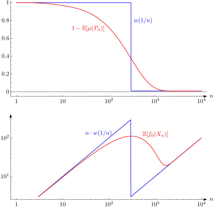 Figure 3
Peer Reviews
No public reviews on file for this paper yet. If you reviewed it on a platform where reviews are public (OpenReview, ICLR, NeurIPS, ICML), you can paste yours below so the community can read it here.
Videos
No videos yet. Explain this paper in a talk, walkthrough, or lecture? Add one.
Random polytopes and the wet part for arbitrary probability distributions
Imre Bárány, Matthieu Fradelizi, Xavier Goaoc, Alfredo Hubard, Günter Rote
Abstract.
We examine how the measure and the number of vertices of the convex hull of a random sample of an arbitrary probability measure in relates to the wet part of that measure.
1. Introduction and Main Results
Let be a convex body (convex compact set with non-empty interior) in , and let be a random sample of uniform independent points from . The set is a random polytope in . For we define the wet part of :
[TABLE]
The name “wet part” comes from the mental picture when is in and contains water of volume . Bárány and Larman [2] proved that the measure of the wet part captures how well approximates in the following sense:
Theorem 1** ([2, Theorem 1]).**
There are constants and depending only on such that for every convex body in and for every
[TABLE]
By Efron’s formula (see (2) below), this directly translates into bounds for the expected number of vertices of , see Section 1.2.
1.1. Results for general measures.
The notions of random polytope and wet part extend to a general probability measure defined on the Borel sets of . The definition of a -random polytope is clear: is a sample of random independent points chosen according to , and . The wet part is defined as
[TABLE]
The -measure of the wet part is denoted by . Here is an extension of Theorem 1 to general measures:
Theorem 2**.**
For any probability measure in and ,
[TABLE]
where as and is independent of .
A similar upper bound, albeit with worse constants, follows from a result of Vu [13, Lemma 4.2], which states that contains with high-probability. Since a containment with high probability is usually stronger than an upper bound in expectation, one may have hoped that the in the upper bound of Theorem 2 can be reduced. Our main result shows that this is not possible, not even in the plane:
Theorem 3**.**
There exists a probability measure on such that
[TABLE]
for infinitely many .
The measure that we construct actually has compact support and can be embedded into for any . It will be apparent from the proof that the same construction has the stronger property that for every constant , the inequality holds for infinitely many values .
1.2. Consequences for -vectors
Let denote the number of vertices of . For non-atomic measures (measures where no single point has positive probability), Efron’s formula [7] relates and :
[TABLE]
For any measure, this still holds as an inequality:
[TABLE]
The measure that is constructed in Theorem 3 is non-atomic. As a consequence, Theorems 2 and 3 give the following bounds for the number of vertices:
Theorem 4**.**
- (i)
For any non-atomic probability measure in ,
[TABLE]
where as and is independent of .
- (ii)
There exists a non-atomic probability measure on such that
[TABLE]
for infinitely many .
Theorem 4 follows from Theorems 2 and 3 except that Efron’s Formula (2) induces a shift in indices, as it relates to . This shift affects only the constant in the lower bound of Theorem 4(i), which goes from to , see Section 3.1.
The upper bound of Theorem 4(i) fails for general distributions. For instance, if is a discrete distribution on a finite set, then for any smaller than the mass of any single point and the upper bound cannot hold uniformly as . Of course, in that case Inequality (3) is strict.
For convex bodies, the number of -dimensional faces of can also be controlled via the measure of the wet part since Bárány [1] proved that for every . No similar generalization is possible for Theorem 2. Indeed, consider a measure in supported on two circles, one on the -plane, the other in the -plane, and uniform on each circle; has edges almost surely.
Before we get to the proofs of Theorems 2 (Section 3.2) and 3 (Section 4), we discuss in Section 2 a key difference between the wet parts of convex bodies and of general measures.
2. Wet part: convex sets versus general measures
A key ingredient in the proof of the upper bound of Theorem 1 in [2] is that for a convex body in , the measure of the wet part cannot change too abruptly as a function of : If , then
[TABLE]
where is a constant that depends only on and [2, Theorem 7]. In particular, a multiplicative factor can be taken out of the volume parameter of the wet part and the upper bound in Theorem 1 can be equivalently expressed as
[TABLE]
(This is in fact how of the upper bound of Theorem 1 is actually formulated in [2, Theorem 1].) This alternative formulation shows immediately that the lower bound of Theorem 1 (and hence also of Theorem 2) cannot be improved by more than a constant.
2.1. Two circles and a sharp drop
The right inequality in (4) does not extend to general measures. An easy example showing this is the following “drop construction”. It is a probability measure in the plane supported on two concentric circles, uniform on each of them, and with measure on the outer circle. Let denote the measure of a halfplane externally tangent to the inner circle; remark that . The measure of the wet part drops at :
[TABLE]
We can make this drop arbitrarily sharp by choosing a small . In particular, for any given , setting makes it impossible to fulfill the right inequality in (4) for .
This example also challenges Inequality (5). As shown in Figure 1 (top), the function has a sharp drop, while shifts from the higher to the lower branch of the step in a gradual way. For this construction, the straightforward extension of Theorem 1 would imply that remains within a constant multiplicative factor of . Thus, would have to follow the steep drop.
2.2. A drop for the number of vertices.
The fact that cannot drop too sharply is more easily seen by examining . Since the measure defined in Equation (6) is non-atomic, Efron’s Formula (2) applies, so let us compare and . As illustrated in Figure 1 (bottom), has a sawtooth shape with a sharp drop from 300 to 3 at , and does actually shift from the higher to the lower branch of the sawtooth, in a gradual way.
The fact that can decrease is perhaps surprising at first sight, but this phenomenom is easy to explain: We pick random points one by one. As long as all points lie on the inner circle, . The first point to fall on the outer circle swallows a constant fraction of the points into the interior of , while adding only a single new point on the convex hull, causing a big drop. This happens around .
Again, the straightforward extension of Theorem 1 would imply that follows the steep drop. Yet, on average, a single additional point can reduce by a factor of at most . Hence, the drop of cannot be so abrupt as the drop of , for small enough.
2.3. A sequence of drops
We prove Theorem 3 in Section 4 by an explicit construction that sets up a sequence of such drops. The function reaches larger and larger peaks as increases, while dropping down more and more steeply between those peaks. Our proof of Theorem 3 will not actually refer to any drop or oscillating behavior. We will simply identify a sequence of values for which is larger than .
2.4. Open questions
It is an outstanding open problem whether a drop as exhibited by our two-circle construction can occur for the uniform selection from a convex body: Can the expectation of the number of vertices of a random polytope decrease in such a setting? This is impossible in the plane [6] or for the three dimensional ball [4], but open in general. See [5] and the discussion therein.
Perhaps Theorem 1 remains valid for some restricted class of measures , for instance, logconcave measures. One approach to circumvent the “impossibility result” of Theorem 3 would be to first extend (4) and establish that for there is such that for all
[TABLE]
The second step would derive from this property the extension of Theorem 1. We don’t know if any of these two steps is valid.
We can weaken the claim of Theorem 1 in a different way, while maintaining it for all measures. For example, it is plausible that the upper bound in the theorem holds for a subset of numbers of positive density. On the other hand we do not know if there is a measure for which the bound of Theorem 1 is valid only for a finite number of natural numbers.
3. Proof of Theorem 2
Let be a probability measure in . For better readability we drop all superscripts .
3.1. Lower bound
The proof of the lower bound is similar to the one in the convex-body case. For every fixed point , by definition, there exists a half-space with and . If is empty, then is not in , and therefore, for ,
[TABLE]
Then, for any ,
[TABLE]
We choose . Since the sequence is increasing, for we have .∎
To obtain the analogous lower bound from Theorem 4(i), we write
[TABLE]
Again, choosing yields the claimed lower bound
[TABLE]
since the sequence is now decreasing to .
3.2. Floating bodies and -nets
Before we turn our attention to the upper bound, we will point out a connection to -nets. Consider a probability space and a family of measurable subsets of . An -net for is a set that intersects every with [10, ]. In the special case where and consists of all half-spaces, if a set is an -net, then the convex hull of contains . Indeed, assume that there exists a point in and not in . Consider a closed halfspace that contains and is disjoint from . Since we must have and cannot be an -net.
We call the region the floating body of the measure with parameter , by analogy to the case of convex bodies. The relation between floating bodies and -nets was first observed by Van Vu, who used the -net Theorem to prove that contains with high probability [13, Lemma 4.2] (a fact previously established by Bárány and Dalla [3] when is the normalized Lebesgue measure on a convex body). This implies that, with high probability, . The analysis we give in Section 3.3 refines Vu’s analysis to sharpen the constant. Note that Theorem 3 shows that Vu’s result is already asymptotically best possible.
3.3. Upper bound
For , the proof of the upper bound is straightforward and may actually be improved. Indeed, we have , and Efron’s Formula (3) yields
[TABLE]
We will therefore assume .
We use a lower bound on the probability of a random sample of to be an -net for . We define the shatter function (or growth function) of the family as
[TABLE]
Lemma 5** ([12, Theorem 3.2]).**
Let be a probability space and a family of measurable subsets of . Let be a sample of random independent elements chosen according to . For any integer , the probability that is not a -net for is at most
[TABLE]
Lemma 5 is a quantitative refinement of a foundational result in learning theory [14, Theorem 2]. It is commonly used to prove that small -nets exist for range spaces of bounded Vapnik-Chervonenkis dimension [9], see also [12, Theorem 3.1] or [11, Theorem 15.5]. For that application, it is sufficient to show that the probability of failure is less than 1; This works for (with appropriate lower-order terms), where is the Vapnik-Chervonenkis dimension. In our proof, we will need a smaller failure probability of order , and we will achieve this by setting . We will apply the lemma in the case where and is the set of halfspaces in . We mention that by increasing more agressively, the probability of failure can be made exponentially small.
For the family of halfspaces in , we have the following sharp bound on the shatter function [8]:
[TABLE]
The proof of the upper bound of Theorem 2 starts by remarking that for any we have:
[TABLE]
Here, the first inequality between the probabilities holds since the event trivially implies that when . We thus have
[TABLE]
We now want to set so that is with as . As shown in Section 3.2, the event implies that fails to be an -net. The probability can thus be bounded from above using Lemma 5 with . Taking logarithms, for any ,
[TABLE]
Since we assume that , we have
[TABLE]
We set , so that:
[TABLE]
We then set , with to be fine-tuned later. If is large enough, the factor is nonnegative, and we can use the inequality for in order to bound the second term:
[TABLE]
Altogether, we get
[TABLE]
so for every we have with as . Setting yields the claimed bound. ∎
4. Proof of Theorem 3
In this section, logarithms are base . For better readability we drop the superscripts .
4.1. The construction
The measure is supported on a sequence of concentric circles , where has radius
[TABLE]
On each , is uniform, implying that is rotationally invariant. We let . For we put
[TABLE]
and remark that , so is a probability measure. The sequence decreases very rapidly. The probabilities of the individual circles are
[TABLE]
for .
The infinite sequence of values for which we claim the inequality of Theorem 3 is
[TABLE]
In Section 4.2, we examine the wet part and prove that . We then want to establish the complementary bound . Since is non-atomic, Efron’s formula yields
[TABLE]
and it suffices to establish that . This is what we do in Section 4.3.
4.2. The wet part
Let us again drop the superscript . Let be a closed halfplane that has a single point in common with , so its bounding line is tangent to . We have
[TABLE]
So, as decreases, drops step by step, each step being from to . In particular,
[TABLE]
For , the portion of contained in is equal to . Hence,
[TABLE]
We will bound the term by a more explicit expression in terms of . To get rid of the function, we use the fact that for all . We obtain, for ,
[TABLE]
Moreover, the ratio can be bounded as follows:
[TABLE]
Thus we deduce that
[TABLE]
We have established a bound on , which is the fraction of a single circle that is contained in . Hence, considering all circles with together, we get
[TABLE]
We check that for ,
[TABLE]
because for all . Using (8), this gives our desired bound:
[TABLE]
for all . With little effort, one can show that actually . One can also see that, for any , the condition holds if is large enough, because the exponential factor dominates any constant factor in the last chain of inequalities. This justifies the remark that we made after the statement of Theorem 3.
4.3. The random polytope
Assume now that is a set of points sampled independently from . We intend to bound from below the expectation . Observe that for any one has
[TABLE]
Intuitively, as varies in the range near , many points of lie on and yet no point of lies in . So has, in expectation, at least vertices. At the same time, the term in the claimed lower bound drops to . So the expected number of vertices is about which is larger than .
Formally, we estimate the expected number of vertices when :
[TABLE]
The last square bracket tends to 1 as . In particular, it is larger than for . This shows that for all
[TABLE]
4.4. Higher dimension
We can embed the plane containing in for . The analysis remains true but the random polytope is of course flat with probability 1. To get a full-dimensional example, we can replace each circle by a -dimensional sphere, all other parameters being kept identical: all spheres are centered in the same point, has radius , the measure is uniform on each and the measure of is . The analysis holds mutatis mutandis.
As another example, which does not require new calculations, we can combine with the uniform distribution on the edges of a regular -dimensional simplex in the -dimensional subspace orthogonal to the plane that contains the circles, mixing the two distributions in the ratio .
In all our constructions, the measure is concentrated on lower-dimensional manifolds of , circles, spheres, or line segments. If a continuous distribution is desired, one can replace each circle in the plane by a narrow annulus and each sphere by a thin spherical shell, without changing the characteristic behaviour.
5. An alternative treatment of atomic measures
Even for measures with atoms, one can give a precise meaning to Efron’s formula: The expression in (1) counts the expected number of convex hull vertices of that are unique in the sample . From this, it is obvious that Efron’s formula (2) is a lower bound on (3).
For dealing with atomic measures, there is alternative possibility. The resulting statements involve different quantities than our original results, but they have the advantage of holding for every measure. We denote by the number of points of the sample that lie on the boundary of their convex hull , counted with multiplicity in case of coincident points. We denote by the interior of . Then a derivation analogous to 1–2 leads to the following variation of Efron’s formula:
[TABLE]
We emphasize that we mean the boundary and interior with respect to the ambient space , not the relative boundary or interior.
Even for some non-atomic measures, this gives different results. Consider the uniform distribution on the boundary of an equilateral triangle. Then , while . Accordingly, , while converges to .
We denote the closure of the wet part by and its measure by .
With these concepts, we can prove the following analogs of Theorems 2–4. Observe that for a measure for which for every hyperplane , the content of this theorem is the same as the previous ones.
Theorem 6**.**
- (i)
For any probability measure in and ,
[TABLE]
and
[TABLE]
where as and is independent of . 2. (ii)
There is a non-atomic probability measure on such that
[TABLE]
and
[TABLE]
for infinitely many .
Proof sketch.
Since the derivation is parallel to the proofs in Sections 3–4, we only sketch a few crucial points.
(i) For proving the lower bound in (10), we modify the initial argument leading to (7): For every fixed , there is a closed half-space with whose corresponding open halfspace has measure . Therefore,
[TABLE]
The remainder of the proof can be adapted in a straightforward way.
In Section 3.2, we have established that for an -net , its convex hull contains . Since the interior operator is monotone, this implies that . Therefore, the -net argument of Section 3.3 applies to the modified setting and establishes the upper bound in (10).
Finally, by Efron’s modified formula (9), the result (10) carries over to (11) as in our original derivation.
(ii) The lower-bound construction of Theorem 3 gives zero measure to every hyperplane, and therefore all quantities in part (ii) are equal to the corresponding quantites in Theorem 3 and Theorem 4(ii). ∎
Acknowledgements.
I. B. was supported by the Hungarian National Research, Development and Innovation Office NKFIH Grants K 111827 and K 116769, and by the Bézout Labex (ANR-10-LABX-58). X. G. was supported by Institut Universitaire de France. The authors are grateful for the hospitality during the ASPAG (ANR-17-CE40-0017) workshop on geometry, probability, and algorithms in Arcachon in April 2018.
The reference list from the paper itself. Each links out to its DOI / PubMed record.
- 1[1] I. Bárány, Intrinsic volumes and f 𝑓 f -vectors of random polytopes, Mathematische Annalen 285 (1989), 671–699.
- 2[2] I. Bárány, D. G. Larman, Convex bodies, economic cap coverings, random polytopes, Mathematika 35 (1988), 274–291.
- 3[3] I. Bárány, L. Dalla, Few points to generate a random polytope, Mathematika 44 (1997), 325–331.
- 4[4] M. Beermann, Random polytopes . Ph. D. thesis, University of Osnabrück, 2015. Available at https://repositorium.ub.uni-osnabrueck.de/bitstream/urn:nbn:de:gbv:700-2015062313276/1/thesis_beermann.pdf .
- 5[5] M. Beermann, M. Reitzner, Monotonicity of functionals of random polytopes . Preprint ar Xiv:1706.08342, (2017).
- 6[6] O. Devillers, M. Glisse, X. Goaoc, G. Moroz, M. Reitzner, The monotonicity of f 𝑓 f -vectors of random polytopes. Electron. Commun. Probab. 18 (2013), 1–8.
- 7[7] B. Efron, The convex hull of a random set of points. Biometrika 52 (1965), 331–343.
- 8[8] E. F. Harding, The number of partitions of a set of n 𝑛 n points in k 𝑘 k dimensions induced by hyperplanes. Proceedings of the Edinburgh Mathematical Society 15(4) (1967), 285–289.