Memory cost of temporal correlations
Costantino Budroni, Gabriel Fagundes, Matthias Kleinmann

TL;DR
This paper investigates the memory cost of simulating temporal correlations in different theories, including classical, quantum, and general probability theories, revealing inequalities that distinguish these correlations.
Contribution
It introduces a theory-independent framework to analyze the memory cost of temporal correlations, extending beyond quantum mechanics to general probability theories.
Findings
Derived inequalities to distinguish classical, quantum, and GPT temporal correlations.
Showed that systems with finite memory capacity can exhibit different temporal correlations.
Provided a unified approach to compare nonclassicality across theories.
Abstract
A possible notion of nonclassicality for single systems can be defined on the basis of the notion of memory cost of classically simulating probabilities observed in a temporal sequence of measurements. We further explore this idea in a theory-independent framework, namely, from the perspective of general probability theories (GPTs), which includes classical and quantum theory as special examples. Under the assumption that each system has a finite memory capacity, identified with the maximal number of states perfectly distinguishable with a single measurement, we investigate what are the temporal correlations achievable with different theories, namely, classical, quantum, and GPTs beyond quantum mechanics. Already for the simplest nontrivial scenario, we derive inequalities able to distinguish temporal correlations where the underlying system is classical, quantum, or more general.
Click any figure to enlarge with its caption.
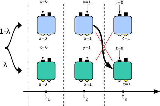 Figure 1
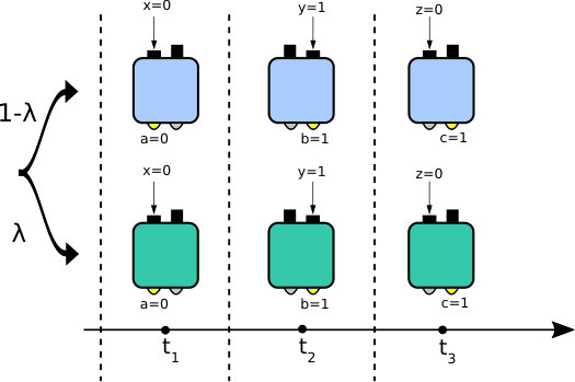 Figure 2
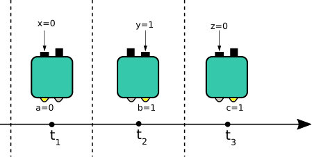 Figure 3
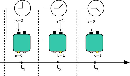 Figure 4
Peer Reviews
No public reviews on file for this paper yet. If you reviewed it on a platform where reviews are public (OpenReview, ICLR, NeurIPS, ICML), you can paste yours below so the community can read it here.
Videos
No videos yet. Explain this paper in a talk, walkthrough, or lecture? Add one.
Memory cost of temporal correlations
Costantino Budroni
Institute for Quantum Optics and Quantum Information (IQOQI), Austrian Academy of Sciences, Boltzmanngasse 3, 1090 Vienna, Austria
Faculty of Physics, University of Vienna, Boltzmanngasse 5, 1090 Vienna, Austria
Gabriel Fagundes
Departamento de Física, Universidade Federal de Minas Gerais UFMG, P.O. Box 702, 30123–970, Belo Horizonte, MG, Brazil
Matthias Kleinmann
Naturwissenschaftlich–Technische Fakultät, Universität Siegen, Walter-Flex-Straße 3, 57068 Siegen, Germany
Abstract
A possible notion of nonclassicality for single systems can be defined on the basis of the notion of memory cost of classically simulating probabilities observed in a temporal sequence of measurements. We further explore this idea in a theory-independent framework, namely, from the perspective of general probability theories (GPTs), which includes classical and quantum theory as special examples. Under the assumption that each system has a finite memory capacity, identified with the maximal number of states perfectly distinguishable with a single measurement, we investigate what are the temporal correlations achievable with different theories, namely, classical, quantum, and GPTs beyond quantum mechanics. Already for the simplest nontrivial scenario, we derive inequalities able to distinguish temporal correlations where the underlying system is classical, quantum, or more general.
I Introduction
Given a single quantum system, in what sense can we say that it has some nonclassical properties? The most celebrated phenomena where quantum systems depart from their classical counterpart involve notions such as entanglement Horodecki et al. (2009); Gühne and Tóth (2009) and nonlocality Bell (1964); Brunner et al. (2014), which can be defined only in terms of multipartite systems. What if we are able to perform experiments only on a single, indivisible, system? Can we still say that the observed statistics has some “nonclassical properties”? Some notion of nonclassicality have been proposed for single systems, such as contextuality Kochen and Specker (1967) and nonmacrorealism Leggett and Garg (1985); Emary et al. (2014). One may argue that such notions are limited to specific measurement procedures and hence are not fully satisfactory. Contextuality restricts the set of possible operations to compatible measurements, which in many cases need to be (approximately) projective or at least satisfy some analogous notion of repeatability and nondisturbance Gühne et al. (2010); Kujala et al. (2015), in order to avoid the so-called “compatibility loophole” Gühne et al. (2010) or other similar classical explanations. Macrorealism has similar strong restrictions on the set of allowed measurements, namely, they must be noninvasive to avoid the clumsiness loophole or other forms of classical interpretation of the results Wilde and Mizel (2012).
A strong motivation for developing such a notion of nonclassicality for single systems also arises from quantum information theory. Notions such as entanglement and nonlocality have been proved to play a role in quantum information tasks related to communication, such as, e.g., device-independent quantum key distribution Acín et al. (2007). That such notions should play a role also for tasks involving only single systems, such as, e.g., quantum computation, is less evident. Several recent results connected quantum contextuality with models of quantum computation such as, e.g., quantum computation via magic state injection or measurement based quantum computation Howard et al. (2014); Delfosse et al. (2015); Raussendorf (2013); Bermejo-Vega et al. (2017); Raussendorf et al. (2017); Abramsky et al. (2017); Oestereich and Galvão (2017). However, a natural question arises of whether this connection is fundamental or just related to the particular model used for quantum computation Markiewicz et al. (2014). If one moves from compatible projective measurements to general instruments, it is no longer clear whether the notion of quantum contextuality make sense at all, due to the compatibility loophole mentioned above Gühne et al. (2010).
In this paper, we go beyond such notions and introduce a notion of nonclassicality for the measurement statistics of a single system which is not restricted to specific measurement operations. The main tool of this investigation is the notion of memory cost of simulating temporal correlations. By temporal correlations we mean the observed statistics arising from sequences of measurements on a single system and memory roughly refers the amount of classical information that can be stored in the physical system.
The notion of memory cost has been explored in connection with classical simulations of quantum contextuality Kleinmann et al. (2011); Fagundes and Kleinmann (2017), quantum simulation of classical stochastic processes Garner et al. (2017) memory asymmetry between prediction and retrodiction Thompson et al. (2018), and in relation with the accuracy of classical and quantum clocks Woods et al. (2018). A related notion, i.e., that of communication cost, has been explored in relation to both Bell nonlocality Pironio (2003); Montina and Wolf (2016) and temporal correlations Brierley et al. (2015); Żukowski (2014). Similar notions have been explored also in the prepare-and-measure scenario Gallego et al. (2010); Brunner et al. (2013); Dall’Arno et al. (2017a, b); Rosset et al. (2018) and in connection with quantum information tasks such as random access codes Bowles et al. (2015); Tavakoli et al. (2016); Aguilar et al. (2018); Miklin et al. (2019).
In our approach, we go beyond the prepare-and-measure scenario by exploring arbitrary long sequences of measurements and we remove any restriction on the type of measurement by considering arbitrary quantum instruments. Our analysis is not only restricted to the differences between classical and quantum theory, but is extended to general probabilistic theories (GPTs) Ludwig (1985); Mittelstaedt (1998); Chiribella et al. (2010); Acín et al. (2010), which embrace also the former theories. In particular, we derive inequalities on the observed probabilities that are able to discriminate between classical, quantum, and genuine GPT correlations. Moreover, as a further development of the ideas presented in Refs. Kleinmann et al. (2011); Fagundes and Kleinmann (2017), we show that in the framework of finite-state machines it is impossible to simulate contextual correlations on a qubit system, for a fixed initial state and arbitrary instruments.
The paper is organized as follows. In Sec. II, we will introduce the basic notions and tools necessary for our analysis, namely, temporal correlations and the arrow of time polytope. In Sec. III, we will introduce finite-state machines in GPTs, in particular, also in classical and quantum theory. In Sec. IV, we will discuss the existence of nontrivial temporal bounds for such theories and the impossibility of simulating contextual correlations on a qubit. Finally, we present the conclusions and an outlook of the paper.
II Temporal correlations
We consider a box that accepts certain inputs from an input alphabet and produces outputs from an output alphabet . The box is operated in a sequential fashion, see Fig. 1(a), such that, for instance, it first receives an input labeled by yielding an output labeled by , subsequently it receives yielding , and finally it receives yielding . Prior to this sequence the box is initialized, such that its behavior is independent of anything except the input sequence . Consequently, for a fixed input sequence , the admissible output sequences are governed by a probability distribution. If we now consider all possible inputs, we obtain the correlations . Due to the time ordering of the inputs and outputs, these correlations must satisfy the arrow of time constraints Clemente and Kofler (2016),
[TABLE]
These constraints encode the fact that a future choice of an input, e.g., or in Eq. (1), must not influence previous outputs of the box, e.g., or . This is in analogy to the nonsignaling conditions in the usual Bell scenario Popescu and Rohrlich (1994). The arrow of time constraints come solely from causality and hence, they must be satisfied not only in classical and quantum theory, but in any GPT.
We can represent the correlations as a vector with coordinates labeled by the possible sequences and . Due to the linearity of the arrow of time constraints, the set of correlations satisfying those forms a polytope. Its extremal points have been recently characterized Abbott et al. (2016); Hoffmann (2016); Hoffmann et al. (2018). It is instructive to briefly sketch the central steps for the simple case of sequences of length three. All correlations in the corresponding polytope can be decomposed as
[TABLE]
since the marginals on the right hand side are well defined (for the pathological cases where we define the right hand side to be zero). Vice versa, taking valid probability distributions , , over , respectively, one always obtains an element of the polytope. Its extremal points are obtained by deterministic strategies, i.e., where each of the probability distributions on the right hand side of Eq. (3) consists only of probabilities [math] or . It easily follows that classical and quantum models can reach extremal points if enough memory is available. In more precise terms, each deterministic strategy can be reached if the box internally keeps a record of all previous inputs and outputs. Storing this record then requires the box to have memory. Of course, the notion of memory needs clarification, in particular if the box is described using quantum theory or a GPT, for details see Sec. III. Clearly, storing the full record of previous inputs and outputs is not necessarily memory optimal and gives rise to the question: What is the minimal number of states necessary to obtain certain correlations? How does such a number depend on the specific theory we use to describe the internals of the box?
An important element, in order to be able to speak about the memory cost of temporal correlations, is the requirement that all time-dependent information used to produce the outputs must be stored within the physical system used to implement the box. This implies that the physical operations performed to produce an output must be time-independent, e.g., the experimenter is not allowed to look at the wall clock and decide to implement in a different way the operation associated with a certain input , as this will result in an additional source of memory, i.e., the clock keeping track of time. It is interesting to notice that the case where such time-dependent are admissible is equivalent to the case of quantum communication scenarios such as quantum random access codes or the scenario described by Brierley et al. Brierley et al. (2015). In fact, the latter scenario can be modeled as a network with ordered nodes, where a single physical system is transmitted through the nodes, and at each time step one of the nodes receives the system, performs a local operation, and transmit the system to the subsequent node. Since for each node it is known in advance in which part of the sequence it is situated, its local operations can be adapted to maximize a certain figure of merit defined in terms of probabilities of outcomes. This scenario covers the notion of “communication cost” and it must be distinguished from the notion of “memory cost” that is considered here. Moreover, even though in the memory cost scenario we are not allowed to change the operations throughout the sequence, it still makes sense to use classical randomness at the beginning of a sequence: at each experimental run, the experimenter can flip a coin and decide to perform the whole sequence of with one box or another. The resulting correlations will be a convex combination of the correlations obtained from either box. A graphical representation of the above ideas is presented in Fig. 1. These intuitive notions are made more rigorous in the next section.
III Finite-state machines
In this section, we formally define the classical, quantum, and GPT models for the box used in the previous section. In this model we assume that the box is implemented as a machine which acts on an internal state. Upon receiving an input , the box operates on the internal state and produces the output . The internal state is the specific model of the memory from the previous section. More precisely, we use the finite number of perfectly distinguishable states as a measure for the memory and for this reason we call this model a finite-state machine.
In a first step we need to describe the internal state and the operations of the machine. We choose ordered vector spaces to describe the machine, which is an appropriate framework for a wide range of GPTs. In Appendix A we give a brief summary of this mathematical formalism. In brief, a GPT is then described by a real vector space with partial order “” and an order unit . In quantum theory would be the set of Hermitian operators, would correspond to being positive semidefinite, and to the identity operator. Measurement outcomes are represented by effects with and a measurement is represented by a collection of effects with . The set of states is a subset of the dual space of such that the probability of outcome in the measurement is given by . Therefore and for all with . The operations represent a specific way to implement a measurement, taking into account the change of the internal state . More precisely, the linear map is such that is the effect describing the output . In addition the positivity condition for any with needs to be satisfied and further restrictions to may apply depending on the specific GPT. If we group together the transformations for a fixed input , then is called an instrument. If we ignore the outcome , then the instrument maps states to states, in the sense that for any state .
Given the initial internal state of the finite-state machine and the instrument , the probabilities associated with a sequence of measurement are given by
[TABLE]
Note, that we write the transformations in the Heisenberg picture, so that the time ordering proceeds from the left to the right. For a general sequence of inputs and outputs we write
[TABLE]
We exemplify in the next sections how this expression is specialized to the classical and quantum case.
As we discussed previously, we exclude any external source of memory, such as a clock keeping track of time. This is formalized by the fact that all instruments solely depend on the input and in particular by the fact that all transformations are time-independent. In general, for a fixed GPT this requirement makes the set of achievable correlations nonconvex. Nevertheless, we can recover convexity by allowing the use of convex mixtures as follows. Before starting the experiment we use a random variable , distributed according to some probability distribution , to decide which finite-state machine to use subsequently. Since the machine is characterized by the initial state and the instruments , this yields the correlations
[TABLE]
The above procedure allows us to generate all correlations from the convex hull of correlations obtainable from a family of finite-state machines parametrized by .
Finally, we define the memory of the system using the GPT notion of capacity (cf. Ref. Masanes and Müller (2011)), i.e., the size of the maximal set of perfectly distinguishable states. More precisely, we say that a GPT defines a -state machine if is the maximal integer such that there exists a collection of states and effects such that
[TABLE]
Namely, all effects are part of the same measurement, which is able to perfectly (i.e., probability one) discriminate among the states. This notion of capacity corresponds to the dimension of the Hilbert space in quantum mechanics and with the number of extremal points of the state simplex in classical probability theory (see, e.g., Ref. Masanes and Müller (2011)).
It is instructive to discuss in more detail the classical and quantum case, which may be more familiar to the reader. We subsequently introduce a particular class of capacity-2 GPTs, the dichotomic norm cones Kleinmann (2014).
III.1 Classical finite-state machines
A classical finite-state machine Paz (2003) is described by its internal rules for state transitions and output probabilities. Given the classical state , the observed probability distribution for an input sequence of length can be written as
[TABLE]
Here, describes the probability of preparing the initial state of the machine111Without loss of generality, we could assume a fixed pure initial state , since we allow for convex mixtures of different machines. Nevertheless, we keep the notation with an initial distribution over all pure states , i.e., a mixed state, to keep the analogy with the standard notation for GPT states () and quantum states (). and describes the probability that the machine yields the output and transition to the state , given that the internal state is and the input is . As in Eq. (6), those machines can depend on a random variable generated at the beginning of each sequence, i.e.,
[TABLE]
For clarity reasons, we use only Eq. (8) in the following. The correlations can be rewritten as
[TABLE]
where is the -dimensional vector of ones, is the vector representing the initial state, and is the transition matrix. Hence, and . The rules for probabilities that constrain translate to for all , and for all .
Translating the above in the languages of GPTs, we let and set the order unit to . The partial order is such that if for all . Then the set of states is given by by the canonical -dimensional simplex,
[TABLE]
In particular is a state. Analogously, the transition matrix corresponds to the instruments , whereas the effects can be obtained as . It can be easily seen that correspond exactly to the capacity defined according to Eq. (7).
III.1.1 Classical finite-state machines and Leggett-Garg’s macrorealist models
It is interesting at this point to briefly compare the model in Eq. (9) with the macrorealist model of Leggett and Garg Leggett and Garg (1985). A macrorealist model can be simply obtained by reducing the set of possible internal states to a single one, i.e., , and re-introducing the time-dependence of operations.
[TABLE]
where the dependency on becomes trivial and is then removed. We recall that macrorealist models are based on two assumptions: macrorealism per se, i.e., the existence of a classical probability, and noninvasive measurability, i.e., the assumption that the measurement has no effect on the subsequent evolution of the system. The finite-state machine model can be seen as arising from the macrorealist model via a relaxation of the assumption of a noninvasive measurement: the measurement can be invasive up to a certain amount quantified by the internal memory of the system, e.g., for a two state-machine the measurement can encode at most one bit of information in the system. Notice that, however, usually Leggett-Garg assumptions allow the operations to be time-dependent.
It is interesting to remark that similar ideas have been already employed in Leggett-Garg tests to tighten the clumsiness loophole. Under the assumption of a classical model with two internal states, Knee et al. Knee et al. (2016) were able to quantify the measurement invasivity via a control experiment, and consequently modify the classical bound for the Leggett-Garg inequality. In agreement with our argument above, the work of Knee et al. shows how the notion of finite memory can be used as a relaxation of the assumption of a noninvasive measurement.
III.2 Quantum finite-state machines
The quantum case is perhaps the most familiar to readers from quantum information. The probability distribution is obtained by sequences of generalized measurements on a single system described by a Hilbert space of fixed dimension . The outcomes of the measurement are described by positive semidefinite operators with .
In order to discuss sequential measurements, however, we need to know the post-measurement state, or, better, the transformation induced by the measurements. This information is provided by a quantum instrument , defined as a collection of completely positive maps , from the space of linear operators into itself, that sum up to a unital map, i.e., , corresponding to the rule of preservation of probability in the Heisenberg picture, see, e.g., Heinosaari and Ziman (2011). Each instrument defines a generalized measurement through the formula . Similarly to the previous cases, we can shorten the notation by defining where denotes the composition of maps and write
[TABLE]
As mentioned before, quantum theory is a particular case of a GPT, where the vectors space is the set of Hermitian operators, the partial order is defined through positive semidefiniteness and the order unit is given by . The set of states is given by the density operators, identified by the Hilbert–Schmidt inner product with the elements of the dual space of ,
[TABLE]
Hence Eq. (13) and Eq. (5) are equivalent. It is then clear that the capacity of the system, defined as the number of perfectly distinguishable state Fritz (2010); Hoffmann et al. (2018) precisely corresponds to the dimension of the Hilbert space. It is important to remark that we need to consider the general formalism of quantum instruments, since if the measurement devices would merely act projectively, there would be nontrivial limitations on the achievable correlations that are valid for arbitrary dimensions Budroni et al. (2013); Budroni and Emary (2014).
III.3 GPT two-state machines
We already provided a definition of GPT finite-state machines at the beginning of Sec. III. In this section, we specialize this definition by considering a class GPTs where the effects belong to a dichotomic norm cone. These theories are a generalization of the classical bit (cbit) and quantum bit (qubit), in the sense that they have capacity two, i.e., they allow for a set of perfectly distinguishable states, in the sense of Eq. (7), of at most size two. We then specialize our discussion to the case of hyperbits (hbits) Pawłowski and Winter (2012) and generalized bits (gbits) Barrett (2007). The former are a generalization of the Bloch sphere to dimension higher than three, whereas the latter are the local part of a Popescu–Rohrlich box Popescu and Rohrlich (1994). We also provide a more detailed discussion of GPTs in Appendix A.
Consider the vector space , and the partial order where if . Here, is any norm in . We define the order unit . This implies that effects are vectors such that . The states for a dichotomic norm cone are the maps with the condition , where is the dual norm of . A peculiarity of this GPT is that it has exactly capacity two, independent of or the choice of the norm . We provide a proof of this fact in Appendix C.
Depending on the norm chosen and on we have different GPTs. If we take to be the Euclidean (or ) norm, i.e., , we obtain hbits, and specifically cbits for , qubits for and more general hbits for . If we take and the Manhattan (or ) norm, i.e., , we obtain a gbit. For the case of the Euclidean norm, the dual norm is also the Euclidean norm itself, whereas the dual of the Manhattan norm is the supremum (or ) norm, i.e., .
IV Bounds on temporal correlations
In this section, we consider the simplest nontrivial scenario, a sequence of two measurements, with inputs and outputs , with . We are interested in bounds on the sum of correlations
[TABLE]
Similar expressions have been considered in Ref. Hoffmann (2016); Hoffmann et al. (2018); Spee et al. (2018). Clearly, the trivial bound holds. For hbits the value cannot be reached and therefore there must exist a nontrivial bound for any dimension of the hbit, in particular for the cbit () and the qubit (). A simple analytical proof of is presented in Appendix B.
IV.1 Measure-and-prepare strategies
The analysis of the case of sequences of length two can be greatly simplified using measure-and-prepare instruments. These are instruments of the form , where is a measurement and is a collection of states. Hence can be implemented by first measuring and then, depending on the outcome , preparing the state .
Now, for a sequence of length two, the correlations are given by
[TABLE]
where is given by the initialization procedure of the individual finite-state machines participating in the mixture of machines. Clearly, the extremal values can be achieved by a single finite-state machine and hence in the following we will omit the index and the summation of .
The instruments can be replaced by measure-and-prepare instruments, by letting and if the denominator is nonzero, or . Then . Hence we can equivalently replace by the prepare-and-measure strategy . Using this simplification, we obtain
[TABLE]
where we used the notation for the probabilities conditioned on previous outputs.
IV.2 Analytical and numerical bounds
Since cannot be reached with hbits, there must be a finite gap between the actual bound for cbits, qubits, and hbits with a Bloch sphere of fixed dimension. In fact, the sets of states and effects are compact, and the expression can be written as a continuous function from the set of states and effects into the interval , so its image must be compact. In this section, we explore in more detail the bounds for cbits, qubits, and hbits via numerical methods.
IV.2.1 Classical bit
For the cbit case, we use the representation from Sec. III.1, specifically, is represented by , by , and by , where . Then Eq. (17) reads
[TABLE]
Only and appear nonlinearly in this expression. Therefore, the maximum of is attained when all remaining parameters are either [math] or . This leaves us with a two-dimensional, at most quadratic optimization, which can be performed at once. For the maximal value of using classical bits we then obtain
[TABLE]
This maximum occurs at a unique point, where , , and . Hence, an optimal machine is given by the initial state and the transition matrices
[TABLE]
Note, that while the solution for the chosen parametrization is unique, the transition matrices are not unique.
IV.2.2 Quantum bit
For the qubit case, we can proceed similarly to Ref. Hoffmann et al. (2018). First we note that in Eq. (17), the initial state can be replaced by a pure state, so that . The expression can then be written as
[TABLE]
where are effects and and are density operators. Since the latter occur only linearly in , we can substitute them with pure states and , respectively. The maximum of for qubits is hence given by
[TABLE]
By parametrizing , , with real parameters, one can write the expression in Eq. (22) as fourth degree polynomial. This can be further simplified, by taking , as real expression, which lowers the number of parameters to ten.222Since the upper bound is calculated by polynomial optimization methods, it is more convenient to keep the expression and constraints in polynomial form, rather than minimizing the number of variables. For example, a parametrization of a pure state as removes one variable and one constraint, but it is no long a polynomial in the parameters. The reduction to the real part of a qubit does not affect the optimality as we show in the next section, see Eq. (28).
It is always possible to obtain a lower bound on by guessing appropriate values for the free parameters. An upper bound, , can be obtained via Lasserre’s method Lasserre (2001) of polynomial optimization based on moment matrices and semidefinite programming (SDP) Vandenberghe and Boyd (1996), which provides analytical upper bounds up to the numerical precision. That is,
[TABLE]
With the simplifications used above, the upper and lower bounds coincide up to the numerical precision of . We have,
[TABLE]
showing a gap between the cbit and qubit case. A feasible solution is given by the post-measurement states and effects,
[TABLE]
and the effects
[TABLE]
IV.2.3 Hyperbit
For the case of hbits, and also the more general dichotomic norm cones, we use the parametrization and for the states and for the effects. Then Eq. (17) reads
[TABLE]
When maximizing , we can eliminate the maximization over and , by choosing appropriate vectors with such that and . The maximal value of for a given dichotomic norm cone is hence
[TABLE]
where the constraints of the optimization are and . For the case of hbits, both and correspond to the norm , hence the conditions are invariant under orthogonal transformations as it is the case for the function to be maximized, which depends only on the norm of and the scalar products between and . Since the only contribution for comes from the component in the span of , the problem reduces to a two-dimensional one. This is equivalent to the qubit case with the Bloch ball restricted to the -plane, both for states and effects. This implies that the bound for hbits coincide with the bound for qubits. We thus have
[TABLE]
as in Eq. (24).
IV.2.4 Generalized bit
The case of gbits differs from the previous one because we can actually reach already for a two-state machine, namely the dichotomic norm cone with and the norm. This model corresponds to the local part of a Popescu–Rohrlich box Popescu and Rohrlich (1994); Barrett (2007). The space of effects is a polytope with extremal effects given by the extremal point of the two-dimensional norm, i.e., , with the canonical vectors in . Then, the states are the with in the square , i.e., the unit ball with respect to the norm. The choices
[TABLE]
and
[TABLE]
yield, according to Eq. (28), the algebraic maximum for , i.e., . We thus have
[TABLE]
for gbits and hence also for the set of all dichotomic norm cones with the same norm and arbitrary .
IV.3 Impossibility of simulating contextual correlations with general
instruments on a qubit
In this section, we investigate whether qubit machines are able to simulate some contextual correlations that arise in higher dimensional quantum systems. In Ref. Kleinmann et al. (2011) it was proved that in order to simulate all deterministic predictions associated with the observables of the Peres–Mermin square Peres (1990); Mermin (1990), a classical machine with at least states is necessary. This result was obtained in the framework of tests of contextuality involving sequential measurements Gühne et al. (2010), in which the relevant compatibility notion is given by the nondisturbance among compatible measurements and repeatability of outcomes, e.g., if and are compatible measurements in the measurement sequence , the outcome for the first measurement of will be repeated in the second measurement of .
We derive here a related result by showing that even a qubit is not sufficient to exhibit contextual correlations. For this we use a rather broad notion of contextuality. Consider a box with inputs from an alphabet and outputs from an alphabet as before. The input sequences are restricted such that a sequence is admissible if and only if all inputs are from the same context , i.e., . A context is a set of inputs, such that for any inputs sequence from , any output sequence , and any permutation . In addition we assume that any input is repeatable, i.e., for any position in any admissible sequence.
Such a box is noncontextual, if all correlations of the box (using only admissible input sequences) can be reproduced by a box without memory, i.e., by a noncontextual model. We claim that any such box implemented on a qubit is noncontextual.
We start the proof of this statement by determining those inputs, which cannot require the use of memory. First, if an input ever produces only the output , within all admissible input sequences, then we can eliminate this input from our considerations. This is the case, because in any sequence we can permute to the end of the sequence. Then
[TABLE]
where the first equality is due to Eq. (3) and the second due to the assumption that only the output ever occurs. Second, assume that for a certain input , whenever it occurs in an admissible sequence, the internal state of the machine before the input is only ever the state . Again we can eliminate this input from our considerations, because the output for and the state after the output can be determined without considering the state. Third, we can ignore the pathological cases of inputs, which are not member of any context. In the following we assume without loss of generality, that the box does not have any input falling under the those three cases just discussed.
Next, we show that for any input the instrument must be a measure-and-prepare instrument of the form
[TABLE]
This can be seen as follows. According to the assumptions, there are two input sequences and and corresponding output sequences and , so that the state before the input is and , respectively, with . Using Eq. (3) and Eq. (13) we have
[TABLE]
where and . Therefore for ,
[TABLE]
with . Since and we assume a qubit system, the mixture has necessarily rank two, i.e., for some . We arrive at the condition
[TABLE]
where and are the Kraus operators associated, respectively, with the instruments and , e.g., . Then for all . Similarly, exchanging with , we obtain for all . This implies that and are of rank one and that is proportional to as well as being proportional to , for all and . Hence we can omit the indices and consider simply and . Note that from , the condition follows which allows us to write with and . Now, for we obtain
[TABLE]
which implies . It follows that either or and are equal up to a phase and hence is as stated in Eq. (34).
As final step we need to show that there is no contextuality for projective qubit instruments. Given an admissible input sequence , and an output sequence such that , we have
[TABLE]
The left hand side of both expressions has to be equal, yielding .
Consequently, any two inputs within a context are realized by the same projective instrument, except for some relabeling of the outcomes. We choose a specific measurement within one context, say , so that with some coefficients . This way we can write for any correlations of this context
[TABLE]
which is exactly the formula for a one-state machine, i.e., a noncontextual model.
This concludes the proof of our statement, due to the following observation. If two contexts share an observable, then our argument already applies and the union of both contexts must admit a noncontextual model and hence the union of both contexts is again a context. Eventually, we can join contexts until all contexts are mutually disjoint. For each disjoint set we can construct a noncontextual model, and since there are no admissible sequence involving two different contexts, we have constructed a noncontextual model for all admissible input sequences.
V Conclusions and outlook
We introduced the notion memory cost of simulating temporal correlations based on the notion of finite-state machine, i.e., a physical system accepting an input at each time instant and generating an outcome and an internal state transition according to probabilistic rules. We investigated the correlations obtainable via such finite-state machines operating according to different probability theories, i.e., classical, quantum, or GPT. Our framework allow us to derive inequalities able to discriminate among different theories for the simplest nontrivial case, i.e., two-state machines, two inputs, two outputs, and sequences of length two. Moreover, we investigated, from the perspective of quantum finite-state machines, the possibility of simulating contextual correlations with a qubit and answered this question in the negative.
Our framework provides a notion of nonclassicality for single systems, which is based solely on observed correlations and does not make any assumption of the type of measurements involved, e.g., compatibility or noninvasiveness. We believe that several problems in quantum foundations and quantum information could be studied in this framework. For instance, a notion of nonclassicality for single systems, i.e., quantum contextuality, has recently been suggested as a resource for quantum computation. On the other hand, memory has been identified as a resource needed to simulate contextual correlations classically Kleinmann et al. (2011); Fagundes and Kleinmann (2017). In addition, a different notion of contextuality for sequential operations has been defined and connected to speed-up in quantum computation Mansfield and Kashefi (2018). Our work could provide a general framework to discuss such different results and understand better the connection between memory cost of (classical) simulations, contextual correlations, and advantages in computation. Moreover, the idea of computation in GPTs, such as Spekkens’ toy model Spekkens (2007), that are intermediate between classical and quantum probability has been recently investigated Johansson and Larsson (2017a, b). In particular, this GPT can be exactly simulated with two classical bits.
Acknowledgements.
The authors would like to thank Rafael Chaves, Andrew Garner, Otfried Gühne, Jannik Hoffmann, Niklas Johansson, Jan-Åke Larsson, Nikolai Miklin, Miguel Navascués, Cornelia Spee, Giuseppe Vitagliano, and Mischa Woods for discussions. This work has been supported by the Austrian Science Fund (FWF): M 2107 (Meitner-Programm) and ZK 3 (Zukunftskolleg), FQXi Large Grant “The Observer Observed: A Bayesian Route to the Reconstruction of Quantum Theory”, FIS2015-67161-P (MINECO/FEDER), Basque Government (project IT986-16), and ERC (Consolidator Grant 683107/TempoQ).
Appendix A Brief introduction to GPTs
In quantum theory the set of effects is represented by Hermitian operators with . This convex set has three characteristic properties. (i) It is a subset of the real vector space of Hermitian operators. (ii) There exists the special operator representing the all-embracing effect. (iii) Its shape is given by the partial order which is defined by the condition that is positive semidefinite.
In a GPT, the notion of an effect is generalized by considering a straightforward generalization of those properties. We start with an arbitrary real vector space with a partial order . This partial order has to be linear in the sense that implies for any and implies if also . This turns into an ordered vector space.
The all-embracing effect is a distinct element . It is is required to dominate all of , i.e., for any there is a positive number such that . This property makes an order unit and an order unit vector space. In addition, it is convenient to assume that the order unit is Archimedean, i.e., if holds for all , then already . In our paper we implicitly assume that any order unit is Archimedean.
It is sometimes convenient to let . Since is equivalent to , we then equivalently describe an AOU space by the tuple . The effects in a GPT are now given by the set . A measurement in a GPT is represented by a collection of elements with , where represent the outcomes of the measurement.
For the set of states, we note that in quantum theory one can represent a state equivalently by the linear map . Then the normalization of becomes and the condition reads for all . By analogy, the set of states in a GPT is given by
[TABLE]
where V^{*}=\set{\varphi\colon V\rightarrow{\mathds{R}}}{\varphi\text{ is linear}} is the dual space of . With this definition, the probability for outcome of a measurement is given by .
Appendix B Bound on for hbits
The proof is by contradiction. Let us assume , we then have , and . From , we have , where . On the other hand, by the definition of effects and state, we have and . We then have
[TABLE]
From (because ), we have and hence . Then, using again and , together with Cauchy–Schwarz inequality, we have
[TABLE]
Similarly, we obtain
[TABLE]
and, again, .
We need now to characterize the terms of the form , corresponding to sequences of length two. We use the constraints that arise from the condition that the transformation must map effects to effects. Then, we use that is a linear transformation that maps the identity element to , i.e., . We, thus, have
[TABLE]
where is a -dimensional vector and a matrix. The expectation value can then be written as
[TABLE]
We can see the transformation , applied to the left, as a state transformation, i.e., Schrödinger picture and with normalization corresponding to outcome probability. Then, we have that . Notice that such a condition also guarantees that and .
This translates to for the case or . In fact, in those cases we have , so the dual norm condition guarantee that for all .
From the conditions , we obtain
[TABLE]
which implies together with Eq. (45), , and Cauchy–Schwarz inequality, that
[TABLE]
On the other hand, we have that, by Eq. (44) and Eq. (52), implies
[TABLE]
which implies , i.e., a contradiction with , which concludes the proof.
Appendix C Capacity of dichotomic norm cones
In the following we prove that dichotomic norm cones describe systems of capacity two. For convenience, we repeat Eq. (7) from the main text.
[TABLE]
We first show that a capacity of two is an upper bound.
Lemma 1**.**
In a dichotomic norm cone, let be a collection of states and a collection of effects, such that Eq. (7) is satisfied. Then .
Proof.
Any effect must satisfy , i.e., and . Furthermore, a state must obey . It follows that and hence requires . Thus implies for the inequalities
[TABLE]
Which yields at once the assertion. ∎
In addition, if the dimension of the underlying vector space is finite, we can always find vectors and , such that , , and . Hence, the states and effects obey Eq. (7). It follows that the capacity of a dichotomic norm cone is always exactly two.
The reference list from the paper itself. Each links out to its DOI / PubMed record.
- 1Horodecki et al. (2009) Ryszard Horodecki, Paweł Horodecki, Michał Horodecki, and Karol Horodecki, “Quantum entanglement,” Rev. Mod. Phys. 81 , 865–942 (2009) . · doi ↗
- 2Gühne and Tóth (2009) Otfried Gühne and Géza Tóth, “Entanglement detection,” Physics Reports 474 , 1 – 75 (2009) . · doi ↗
- 3Bell (1964) John Stewart Bell, “On the Einstein-Podolsky-Rosen paradox,” Physics 1 , 195–200 (1964) .
- 4Brunner et al. (2014) Nicolas Brunner, Daniel Cavalcanti, Stefano Pironio, Valerio Scarani, and Stephanie Wehner, “Bell nonlocality,” Rev. Mod. Phys. 86 , 419–478 (2014) . · doi ↗
- 5Kochen and Specker (1967) Simon Kochen and Ernst P. Specker, “The problem of hidden variables in quantum mechanics,” J. Math. Mech. 17 , 59 (1967) .
- 6Leggett and Garg (1985) Anthony J. Leggett and Anupam Garg, “Quantum mechanics versus macroscopic realism: Is the flux there when nobody looks?” Phys. Rev. Lett. 54 , 857–860 (1985) . · doi ↗
- 7Emary et al. (2014) Clive Emary, Neill Lambert, and Franco Nori, “Leggett–Garg inequalities,” Reports on Progress in Physics 77 , 016001 (2014) .
- 8Gühne et al. (2010) Otfried Gühne, Matthias Kleinmann, Adán Cabello, Jan-Åke Larsson, Gerhard Kirchmair, Florian Zähringer, Rene Gerritsma, and Christian F. Roos, “Compatibility and noncontextuality for sequential measurements,” Phys. Rev. A 81 , 022121 (2010) . · doi ↗