Well-posedness of a non-local model for material flow on conveyor belts
Elena Rossi (Acumes), Jennifer K\"otz, Paola Goatin (Acumes), Simone, G\"ottlich

TL;DR
This paper investigates finite volume schemes for a non-local two-dimensional material flow model, proving convergence, stability, and comparing Roe-type and Lax-Friedrichs discretizations through numerical analysis.
Contribution
It introduces a convergence proof for finite volume schemes applied to a non-local flow model, including a comparison of Roe and Lax-Friedrichs methods and establishing solution uniqueness.
Findings
Roe scheme offers benefits over Lax-Friedrichs in numerical simulations.
Convergence of approximate solutions is proven despite flux discontinuities.
Solution depends continuously on initial data, ensuring uniqueness.
Abstract
In this paper, we focus on finite volume approximation schemes to solve a non-local material flow model in two space dimensions. Based on the numerical discretisation with dimensional splitting, we prove the convergence of the approximate solutions, where the main difficulty arises in the treatment of the discontinuity occurring in the flux function. In particular, we compare a Roe-type scheme to the well-established Lax-Friedrichs method and provide a numerical study highlighting the benefits of the Roe discretisation. Besides, we also prove the L1-Lipschitz continuous dependence on the initial datum, ensuring the uniqueness of the solution.
Click any figure to enlarge with its caption.
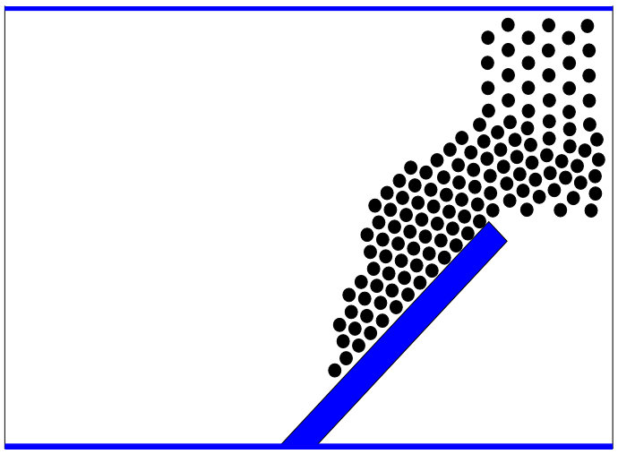 Figure 1
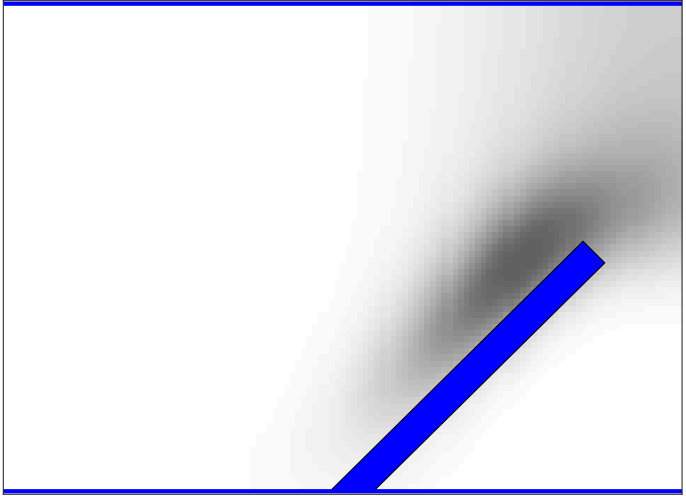 Figure 2
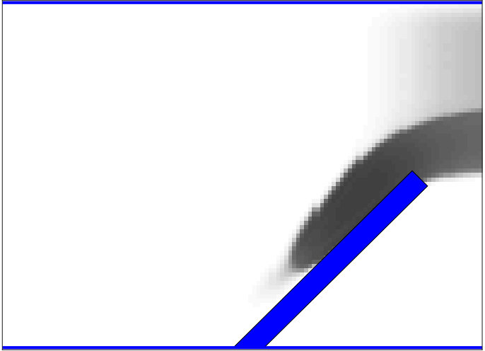 Figure 3
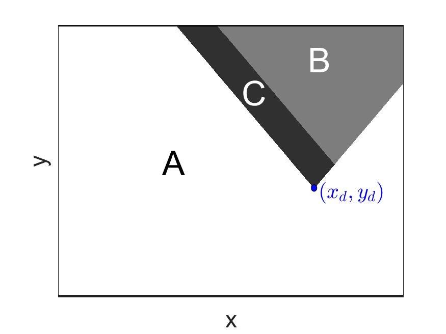 Figure 4
| Approximation | [m] | CFL time step Roe [s] | CFL time step LxF [s] | |
|---|---|---|---|---|
| (atan) | ||||
| (polynomial) |
| CFL time step | -error | -error | -error | |
|---|---|---|---|---|
Peer Reviews
No public reviews on file for this paper yet. If you reviewed it on a platform where reviews are public (OpenReview, ICLR, NeurIPS, ICML), you can paste yours below so the community can read it here.
Videos
No videos yet. Explain this paper in a talk, walkthrough, or lecture? Add one.
Well–posedness of a non-local model for material flow
on conveyor belts
Elena Rossi111Inria Sophia Antipolis - Méditerranée, Université Côte d’Azur, Inria, CNRS, LJAD, 2004 route des Lucioles - BP 93, 06902 Sophia Antipolis Cedex, France. E-mail: {elena.rossi, paola.goatin}@inria.fr
Jennifer Kötz222University of Mannheim, Department of Mathematics, 68131 Mannheim, Germany. Email: [email protected], [email protected]
Paola Goatin111Inria Sophia Antipolis - Méditerranée, Université Côte d’Azur, Inria, CNRS, LJAD, 2004 route des Lucioles - BP 93, 06902 Sophia Antipolis Cedex, France. E-mail: {elena.rossi, paola.goatin}@inria.fr
Simone Göttlich222University of Mannheim, Department of Mathematics, 68131 Mannheim, Germany. Email: [email protected], [email protected]
Abstract
In this paper, we focus on finite volume approximation schemes to solve a non-local material flow model in two space dimensions. Based on the numerical discretisation with dimensional splitting, we prove the convergence of the approximate solutions, where the main difficulty arises in the treatment of the discontinuity occurring in the flux function. In particular, we compare a Roe-type scheme to the well-established Lax-Friedrichs method and provide a numerical study highlighting the benefits of the Roe discretisation. Besides, we also prove the -Lipschitz continuous dependence on the initial datum, ensuring the uniqueness of the solution.
Keywords: non-local conservation laws; material flow; Roe scheme; Lax-Friedrichs scheme
2010 Mathematics Subject Classification: 35L65, 65M12
1 Introduction
In this paper, we consider the Cauchy problem for a non-local scalar conservation law in two space dimensions, namely
[TABLE]
for any , where for the weighting factor
[TABLE]
Here, denotes the Heaviside function which becomes active whenever the maximal density is exceeded.
The above model was introduced in [9], to describe the flow of objects on a conveyor belt. In particular, the unknown function is the density of transported parts, is the velocity vector field induced by the conveyor belt, which is constant in time. So, below the maximal density, parts are transported with the velocity of the conveyor belt. On the other hand, the dynamic velocity vector field is active only at high densities and accounts for colliding parts through the operator . The negative gradient of the convolution pushes the mass towards lower density regions. The particular choice of the collision operator was introduced in [5] to describe crowd dynamics.
Conservation laws with non-local flux function have been recently introduced in the literature to describe transport phenomena accounting for non-local interaction effects among agents, such as road traffic flow [3] or pedestrian dynamics [5]. General well-posedness results have been provided by [2] in the scalar one-dimensional case, while [1] deals with systems of non-local conservation laws in multi-space dimensions. Even if the latter result applies to our problem (1.1), estimates in [1] where obtained for general flux functions using finite volume approximate solutions constructed via Lax-Friedrichs scheme. The aim of the present paper is instead to derive sharp estimates for the Roe scheme, which is known to give less diffusive solutions and is therefore computationally more convenient, especially in the case of non-local problems in multi-D. The same remark holds for the -stability estimates, which have been derived from scratch even if more general results are present in the literature [12, 13].
We finally remark that, even if the original model proposes the use of the discontinuous Heaviside function, the stability of the numerical schemes requires a smooth approximation of it. Indeed, it can be noticed that -norm of the derivative appears in the estimates (for instance in the CFL condition (3.9) that guarantees the -estimates), which blow up with it.
The paper is organised as follows: for a better overview, we introduce our main results in Section 2 and start then to prove convergence of the approximate solution constructed by the Roe scheme in Section 3. We also add a proof of the Lipschitz continuous dependence on the initial data in Section 4. Sections 5 and 6 are devoted to the comparison of results obtained by the Lax-Friedrichs method. The numerical results emphasise the good performance of the Roe scheme.
2 Main results
Throughout the paper, we will denote , for any . We require the following assumptions to hold:
.
The function is a smooth approximation of the Heaviside function such that, setting
[TABLE]
the function has bounded derivative. In particular, we denote by the Lipschitz constant of the function :
[TABLE]
.
Recall the definition of solution to the Cauchy problem (1.1), see also [1, 2, 5].
Definition 2.1**.**
Let . A map is a solution to (1.1) if it is a Kružkov solution to
[TABLE]
with .
Above, for the definition of Kružkov solution we refer to [11, Definition 1].
Theorem 2.2**.**
Let . Let assumptions , and hold. Then, for all , there exists a unique weak entropy solution to problem (1.1). Moreover, the following estimates hold: for all
[TABLE]
where is defined in (3.12), is defined in (3.16), is defined in (3.17) and is as in (3.38).
The proof of Theorem 2.2 is standard, see [1, Theorem 2.3], which refers to [15]. The uniqueness is ensured by Proposition 4.1, which provides the Lipschitz continuous dependence estimate of solutions to (1.1) on the initial data.
The bounds presented in Theorem 2.2 are obtained by passing to the limit in the corresponding discrete bounds.
3 Existence
Introduce the uniform mesh of width along the -axis and along the -axis, and a time step subject to a CFL condition, specified later on. For set
[TABLE]
where and denote the cells interfaces and are the cells centres. Set and let , , be the time mesh. Set and , and let be the viscosity coefficients.
For the sake of shortness, sometimes we will use also the notation .
We approximate the initial datum as follows: for
[TABLE]
and we define a piece-wise constant solution to (1.1) as
[TABLE]
through a modified Roe-type scheme with dimensional splitting, exactly as in [9]:
Algorithm 3.1**.**
[TABLE]
Above, we set and the convolution products are computed through the following quadrature formula, for ,
[TABLE]
where and . Remark that the choice of evaluating the numerical flux at for both fractional steps allows to save computational time, because the convolution products (3.7) are computed only once per time step.
Introduce the following notation, which is of use below:
[TABLE]
3.1 Positivity
In the case of positive initial datum, we prove that under a suitable CFL condition the approximate solution to (1.1) constructed via the Algorithm 3.1 preserves the positivity.
Lemma 3.2**.**
(Positivity)* Let . Let , , and hold. Assume that*
[TABLE]
Then, for all and , the piece-wise constant approximate solution (3.1) constructed through Algorithm 3.1 is such that .
Proof. Fix between [math] and and assume that for all . Consider (3.5), with the notation (3.2) and (3.3), and observe that:
[TABLE]
Therefore, by (3.5),
[TABLE]
thanks to the CFL condition (3.9). Starting from (3.6), an analogous argument shows that , concluding the proof.
3.2 bound
The following result on the bound follows from the conservation property of the Roe scheme.
Lemma 3.3**.**
( bound)* Let . Let , , and (3.9) hold. Then, for all and , (3.1) constructed through Algorithm 3.1 satisfies*
[TABLE]
3.3 bound
Lemma 3.4**.**
( bound)* Let . Let , , and (3.9) hold. Then, for all and , (3.1) constructed through Algorithm 3.1 satisfies*
[TABLE]
where
[TABLE]
Proof. Omitting the dependencies on and exploiting the notation introduced in (3.8), we
observe that (3.5) attains its maximum for , , and . In this case
[TABLE]
where we use the positivity of each and of the function and discard all the terms giving a negative contribution. Moreover, since and ,
[TABLE]
with . In a similar way, since and , exploiting also the fact that for all , we get
[TABLE]
thanks to (A.2). Therefore,
[TABLE]
In a similar way we get
[TABLE]
concluding the proof.
3.4 bound
Proposition 3.5**.**
( estimate in space)* Let . Let , , and hold. Assume that*
[TABLE]
Then, for all , in (3.1) constructed through Algorithm 3.1 satisfies the following estimate: for all ,
[TABLE]
where
[TABLE]
with
[TABLE]
and are defined in (A.6).
Remark 3.6**.**
Observe that the CFL conditions (3.13) are stricter than (3.9).
Proof. We follow the idea of [1, Lemma 2.7]. First consider the term
[TABLE]
In particular, fixing and omitting the dependencies on for the sake of simplicity, by (3.5) we get
[TABLE]
where we set
[TABLE]
For the sake of shortness, introduce the following notation
[TABLE]
so that, dropping the dependencies, reads
[TABLE]
where
[TABLE]
Exploiting (3.18), observe that, whenever ,
[TABLE]
with . Since and by (3.13) we get
[TABLE]
In a similar way one can prove that . Thus,
[TABLE]
We pass now to . Consider separately the terms involving and those involving . Observe that the maps
[TABLE]
are Lipschitz continuous, with constant respectively and . Exploiting (3.2) we get:
[TABLE]
since
[TABLE]
with and .
Similarly, exploiting (3.3) we obtain
[TABLE]
where we used the fact that , (A.2) and (A.4), with the notation (A.6). Collecting together (3.22) and (3.23) we therefore obtain
[TABLE]
so that
[TABLE]
Therefore, by (3.21) and (3.24), using also Lemma 3.3
[TABLE]
Now pass to the term
[TABLE]
Fix and exploit (3.5) again to get
[TABLE]
where we set
[TABLE]
[TABLE]
Similarly as before, rearrange , exploiting the notation (3.18):
[TABLE]
where
[TABLE]
As for (3.19) and (3.20), it is immediate to prove that for all . Hence,
[TABLE]
Pass now to : we can proceed analogously to , treating separately the terms involving and those involving . First, by (3.2),
[TABLE]
since
[TABLE]
with and . In a similar way, by (3.3),
[TABLE]
where we used the fact that , (A.3) and (A.5), with the notation (A.6). Therefore, collecting together (3.27) and (3.28), we get
[TABLE]
so that
[TABLE]
Hence, by (3.26) and (3.29), using also Lemma 3.3, we obtain
[TABLE]
Setting
[TABLE]
by (3.25) and (3.30) we conclude
[TABLE]
Analogous computations yield
[TABLE]
where
[TABLE]
Observe that, using the notation (3.16) and (3.17),
[TABLE]
A recursive argument yields the desired result:
[TABLE]
Corollary 3.7**.**
( estimate in space and time)*
Let . Let , , , (3.13) hold. Then, for all , in (3.1) constructed through Algorithm 3.1 satisfies the following estimate: for all ,*
[TABLE]
where
[TABLE]
with as in (3.15) and as in (3.38).
Proof. By Proposition 3.5 we have
[TABLE]
Since
[TABLE]
we focus first on
[TABLE]
By the scheme (3.5), we have, using the notation (3.8),
[TABLE]
where and we used , (A.1) and (A.2). Therefore,
[TABLE]
where we set
[TABLE]
Analogously, we get
[TABLE]
Hence
[TABLE]
which together with (3.37) completes the proof.
3.5 Discrete entropy inequalities
Following [1], see also [7, 8], introduce the following notation: for , and ,
[TABLE]
with , and defined as in (3.2), (3.4) and (3.3) respectively.
Lemma 3.8**.**
(Discrete entropy condition)*
Fix . Let , , , (3.13) hold. Then, the solution in (3.1) constructed through Algorithm 3.1 satisfies the following discrete entropy inequality: for , for and ,*
[TABLE]
The proof is omitted, being entirely analogous to that of [2, Proposition 2.8], see also [1, Lemma 2.8].
4 Lipschitz continuous dependence on initial data
Proposition 4.1**.**
Fix . Let , and hold. Let . Call and the corresponding solutions to (1.1). Then the following estimate holds:
[TABLE]
with defined in (4.2).
Proof. In the rest of the proof, to avoid heavy notation, we will denote pairs in by or . Introduce the following notation:
[TABLE]
The idea is to apply the doubling of variables method introduced by Kružkov in [11], exploiting in particular the proof of [4, Lemma 4]. There, a flux of the form is taken into account, with , the proof being valid also in the multidimensional case, i.e. . Therefore we are going to use this result for what concerns the part of the flux of type .
For the sake of completeness, we recall that a flux function of type is considered in [10], with , and the proof of [4, Lemma 4] follows the lines of that of [10, Theorem 1.3]. Thus, here we are adding the dependence on time to the function considered in [10].
Let be a test function as in the definition of solution by Kružkov. Let be such that
[TABLE]
Define, for , . Clearly, , , for , and as , being the Dirac delta in [math]. Define moreover
[TABLE]
Introduce the space and, from the definition of solution, derive the following entropy inequalities for and :
[TABLE]
Sum the two inequalities above and rearrange the terms therein, following the proof of [11, Theorem 1] for what concerns the linear part of the flux and the proof of [4, Lemma 4], see also [10, Theorem 1.3], for the other part:
[TABLE]
Let , which gives
[TABLE]
Choosing a suitable test function leads to
[TABLE]
Observe that, following [6, Lemma 4.1], the following bounds hold
[TABLE]
Thus, letting and exploiting the bounds on and given by Theorem 2.2, as well as , we get
[TABLE]
with
[TABLE]
An application of Gronwall Lemma, together with
[TABLE]
yields the desired estimate
[TABLE]
Remark 4.2**.**
We can interpret and as solutions of the following Cauchy problems:
[TABLE]
where
[TABLE]
so that the distance between the solutions at time can be estimated by [12, Proposition 2.10], see also the refinement in [13, Proposition 2.9]. However, making use of the explicit expression of the flux in the present case, one may see that the bound provided by Proposition 4.1 is sharper than that coming from [13, Proposition 2.9].
5 Lax–Friedrichs scheme
It is also possible to consider a piece-wise constant solution to (1.1) as in (3.1) defined through a Lax–Friedrichs type finite volume scheme with dimensional splitting. The algorithm reads as follows
Algorithm 5.1**.**
[TABLE]
The algorithm is close to that studied in [1], except that in the present case to compute the flux is evaluated at , instead of .
Following closely the proofs presented in [1], it is possible to recover also for Algorithm 5.1 the bounds on the approximate solution necessary to prove the convergence. Below, we state only the final results, omitting the computations.
Lemma 5.2**.**
(Positivity)*
Let . Let assumptions , and hold. Assume that*
[TABLE]
Then, for all and , the piece-wise constant approximate solution (3.1) constructed through Algorithm 5.1 is such that .
Lemma 5.3**.**
( bound)*
Let . Let , , , (5.5) and (5.6) hold. Then, for all , in (3.1) constructed through Algorithm 5.1 satisfies (3.10), that is*
[TABLE]
Lemma 5.4**.**
( bound)*
Let .Let , , , (5.5) and (5.6) hold. Then, for all , in (3.1) constructed through Algorithm 5.1 satisfies*
[TABLE]
where
[TABLE]
Remark 5.5**.**
Compare the estimate obtained in Lemma 5.4 using the Lax–Friedrichs scheme with that in Lemma 3.4, given by the Roe scheme. Although they look very similar, the constants appearing in the exponent are actually different: when comparing above to as in (3.12), we see that in the last addend is multiplied by .
Proposition 5.6**.**
( estimate in space)*
Let . Let , , , (5.5) and (5.6) hold. Then, for all , in (3.1) constructed through Algorithm 5.1 satisfies the following estimate: for all ,*
[TABLE]
where
[TABLE]
with
[TABLE]
* as in (3.17) and are defined in (A.6).*
Remark 5.7**.**
Observe that in (3.16).
Corollary 5.8**.**
( estimate in space and time)*
Let . Let , , , (5.5) and (5.6) hold. Then, for all , in (3.1) constructed through Algorithm 5.1 satisfies the following estimate: for all ,*
[TABLE]
where
[TABLE]
with as in (5.7) and
[TABLE]
6 Numerical results
We consider the test setting given in [9] to compare the results of the Roe scheme, cf. Algorithm 3.1, to the results of the Lax-Friedrichs type scheme, cf. Algorithm 5.1.
6.1 Test setting
A total number of parts in the shape of metal cylinders are transported on a conveyor belt moving with speed 0.42 m/s and are redirected by a diverter. The diverter is positioned at an angle of degree with respect to the border of the conveyor belt. Figure 1 illustrates the static velocity field of the conveyor belt. Parts are transported with velocity in Region A and the diverter redirects the parts (Region C). The area behind the diverter (Region B) is modelled in a way that should prohibit parts from passing through the diverter, see [9]. The point marks the end of the diverter.
6.2 Discretisation and solution properties
To numerically model the setting, we introduce a uniform grid on the selected area of the conveyor belt. Initial conditions for the density at time are given by the experimental data and normalised so that . The mollifier which is used in the operator (1.2) is chosen as follows
[TABLE]
with .
In the original model formulation [9], the Heaviside function was introduced to avoid densities larger than . In this work, we investigate the performances of two numerical schemes with two types of smooth approximations of the Heaviside function, one sensibly closer than the other. The former is the approximation (atan), obtained using the inverse tangent
[TABLE]
while the latter is denoted (polynomial) and it is obtained by cubic spline interpolation with the following conditions
[TABLE]
The approximation for and together with the inverse tangent approximation are depicted in Figure 2.
Using the inverse tangent approximation corresponds to activating the collision operator very close to . On the other hand, with the polynomial approximation, the collision operator starts activating at , which implies that clusters with densities values between and are already dispersed to some extent. Numerically, this means that densities above the maximum one are more likely to appear when using the inverse tangent approximation, while exploiting the polynomial approximation prevents from reaching such high values of the density.
Clearly, different approximations of the Heaviside function lead to different Lipschitz constants (2.1) and therefore influence the CFL time steps of the Roe scheme (3.13) and of the Lax-Friedrichs scheme (5.5)–(5.6). Moreover, the constants and given by the CFL condition for the Lax-Friedrichs scheme depend on the Lipschitz constant . Larger Lipschitz constants, and therefore higher viscosity coefficients and , add additional viscosity to the Lax-Friedrichs scheme and therefore more diffusion, as shown in [14]. Note that in general, the Lax-Friedrichs scheme is more diffusive than the Roe scheme. To ensure conservation of mass within the given area of the conveyor belt, we impose zero–flux–conditions at the boundaries of the conveyor belt for the Lax-Friedrichs scheme. Therefore, at the boundary, the flux that would exit the domain is set to zero.
The Lipschitz constants of the approximations of the Heaviside functions depicted in Figure 2, as well as the corresponding CFL conditions, are displayed in Table 1, for a fixed space step size . The inverse tangent approximation has a greater Lipschitz constant, leading to small CFL time steps and thus to an increased computational effort.
We analyze the amount of parts that pass the obstacle, i.e. the outflow at the end of the obstacle . The time-dependent mass function counts the measured parts that are located in the region
[TABLE]
where is the left sided region upstream the obstacle and is the position of part , , at time . The time-dependent mass function describing the outflow to the solution of the conservation law is given by
[TABLE]
The outflow curves obtained using Roe scheme, Lax-Friedrichs scheme and the outflow measured experimentally are shown in Figure 4. The parameters chosen for each scheme are those given in Table 1. Figure 4 displays the norms of the solution over time.
The outflow curve given by Roe scheme for both approximations of the Heaviside function is closer to the experimental data, due to the fact that the scheme captures more congestion, as indicated also by the norm. With Roe scheme, as expected, the density piles up even more when using the inverse tangent approximation. We observe that a maximum principle is not verified. On the contrary, with the polynomial approximation, higher densities are avoided, since the collision operator is activated earlier. Due to the influence of the viscosity coefficients, an opposite behaviour is observable with the Lax-Friedrichs scheme. Results for the norm of the solution are quite promising using the polynomial approximation, whereas the viscosity of the scheme is too large in the case of the inverse tangent approximation. The norm of the solution is constantly decreasing over time because of diffusion.
Figure 5 displays the parts’ positions in the experiment and the density distribution computed with Roe and Lax-Friedrichs scheme using the polynomial Heaviside approximation at time . The density plot of the Roe scheme matches the experimental data quite well: regions with higher densities mostly coincide with regions in the experiments, where the parts are side by side. In contrast, the Lax-Friedrichs scheme produces a more widely spread density distribution. Even the parts on the upper section of the belt, which are transported to the right with the velocity of the conveyor belt, are not correctly portrayed.
Since the Roe scheme using the sharper approximation of the Heaviside function provides the best result in comparison to the experimental data, we analyse its behaviour for . Table 2 shows the error norms of the outflow of the simulations with the Roe scheme and the inverse tangent approximation of the Heaviside function compared to to the outflow given by the experimental data.
The scheme is evaluated for different space step sizes and their corresponding CFL time steps. We observe that the error of the Roe scheme decreases as the space step decreases, suggesting the convergence of the outflow to the experimental data, compare also Figure 6.
Acknowledgments
This work was financially supported by the project “Non-local conservation laws for engineering applications” co-funded by DAAD (Project-ID 57445223) and the PHC Procope (Project no. 42503RM) and the DFG project GO 1920/7-1. Elena Rossi was partially supported by University of Mannheim and acknowledges its hospitality during the accomplishment of this work.
Appendix A Technical Lemma
Lemma A.1**.**
Let . Then, for , for , the following estimates hold:
[TABLE]
where we set
[TABLE]
Proof. The proof of (A.1) is immediate.
Pass now to (A.2). For the sake of simplicity, introduce the following notation:
[TABLE]
Hence,
[TABLE]
Consider (A.8): since and
[TABLE]
we obtain
[TABLE]
On the other hand, to estimate (A.9), compute
[TABLE]
Introduce and , for . In particular compute and observe that . Then
[TABLE]
Therefore,
[TABLE]
Inserting (A.10) and (A.12) into the estimate of (A.7) yields the desired result.
Consider now (A.4). Introduce the following notation: for set
[TABLE]
Thus
[TABLE]
Consider the terms separately, forgetting for a moment the in front of everything. Focus first on the terms with common denominator :
[TABLE]
with . We are left with
[TABLE]
Add and subtract to (A.14)
[TABLE]
Hence,
[TABLE]
Consider first (A.16): exploiting also (A.11), we obtain
[TABLE]
As far as (A.15) is concerned, focus on the terms in the brackets:
[TABLE]
Inserting the first addend of (A.18) back into (A.15) yields
[TABLE]
where we exploit (A.11) twice and use the fact that . Concerning the second addend of (A.18), focus on its numerator: with the notation introduced before (A.11),
[TABLE]
where and . Now insert this estimate back into (A.18) and (A.15): since ,
[TABLE]
Collecting together (A.13), (A.17), (A.19) and (A.20) yields
[TABLE]
The reference list from the paper itself. Each links out to its DOI / PubMed record.
- 1[1] A. Aggarwal, R. M. Colombo, and P. Goatin. Nonlocal systems of conservation laws in several space dimensions. SIAM J. Numer. Anal. , 53(2):963–983, 2015.
- 2[2] P. Amorim, R. M. Colombo, and A. Teixeira. On the numerical integration of scalar nonlocal conservation laws. ESAIM Math. Model. Numer. Anal. , 49(1):19–37, 2015.
- 3[3] S. Blandin and P. Goatin. Well-posedness of a conservation law with non-local flux arising in traffic flow modeling. Numer. Math. , 132(2):217–241, 2016.
- 4[4] F. A. Chiarello, P. Goatin, and E. Rossi. Stability estimates for non-local scalar conservation laws. Nonlinear Anal. Real World Appl. , 45:668–687, 2019.
- 5[5] R. M. Colombo, M. Garavello, and M. Lécureux-Mercier. A class of nonlocal models for pedestrian traffic. Math. Models Methods Appl. Sci. , 22(4):1150023, 34, 2012.
- 6[6] R. M. Colombo and E. Rossi. Hyperbolic predators vs. parabolic prey. Commun. Math. Sci. , 13(2):369–400, 2015.
- 7[7] M. Crandall and A. Majda. The method of fractional steps for conservation laws. Numer. Math. , 34(3):285–314, 1980.
- 8[8] M. G. Crandall and A. Majda. Monotone difference approximations for scalar conservation laws. Math. Comp. , 34(149):1–21, 1980.