$^{60}$Fe in core-collapse supernovae and prospects for X-ray and $\gamma$-ray detection in supernova remnants
Samuel Jones, Heiko Moeller, Chris L. Fryer, Christopher J. Fontes,, Reto Trappitsch, Wesley P. Even, Aaron Couture, Matthew R. Mumpower, Samar, Safi-Harb

TL;DR
This paper studies $^{60}$Fe production in supernovae, its detection prospects in gamma-ray and X-ray spectra, and implications for understanding supernova remnants and solar system formation.
Contribution
It provides new insights into $^{60}$Fe yields dependence on nuclear reaction rates and explores detection strategies for supernova remnants via gamma-ray and X-ray observations.
Findings
$^{60}$Fe yield increases with $^{59}$Fe$(n, extgamma)^{60}$Fe cross section.
Most models cannot explain Solar System $^{60}$Fe origin.
Next-generation gamma-ray telescopes could detect up to 100 old SNRs.
Abstract
We investigate Fe in massive stars and core-collapse supernovae focussing on uncertainties that influence its production in 15, 20 and 25 stars at solar metallicity. We find that the Fe yield is a monotonic increasing function of the uncertain FeFe cross section and that a factor of 10 reduction in the reaction rate results in a factor 8-10 reduction in the Fe yield; while a factor of 10 increase in the rate increases the yield by a factor 4-7. We find that none of the 189 simulations we have performed are consistent with a core-collapse supernova triggering the formation of the Solar System, and that only models using FeFe cross section that is less than or equal to that from NON-SMOKER can reproduce the observed Fe/Al line flux ratio in the diffuse ISM. We examine the prospects of detecting…
Click any figure to enlarge with its caption.
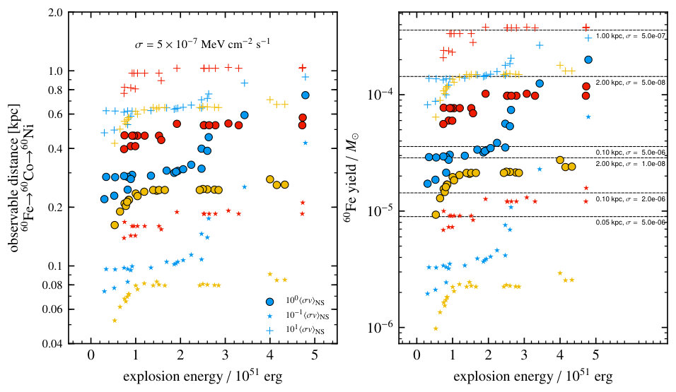 Figure 1
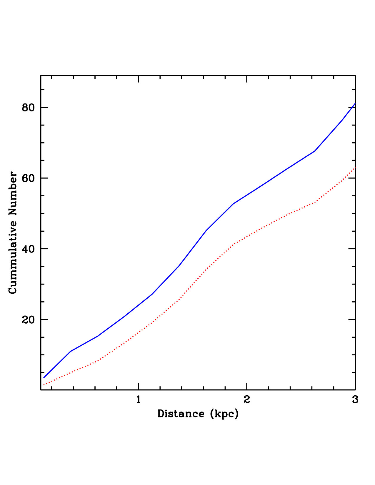 Figure 2
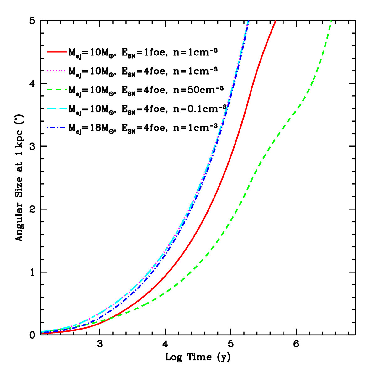 Figure 3
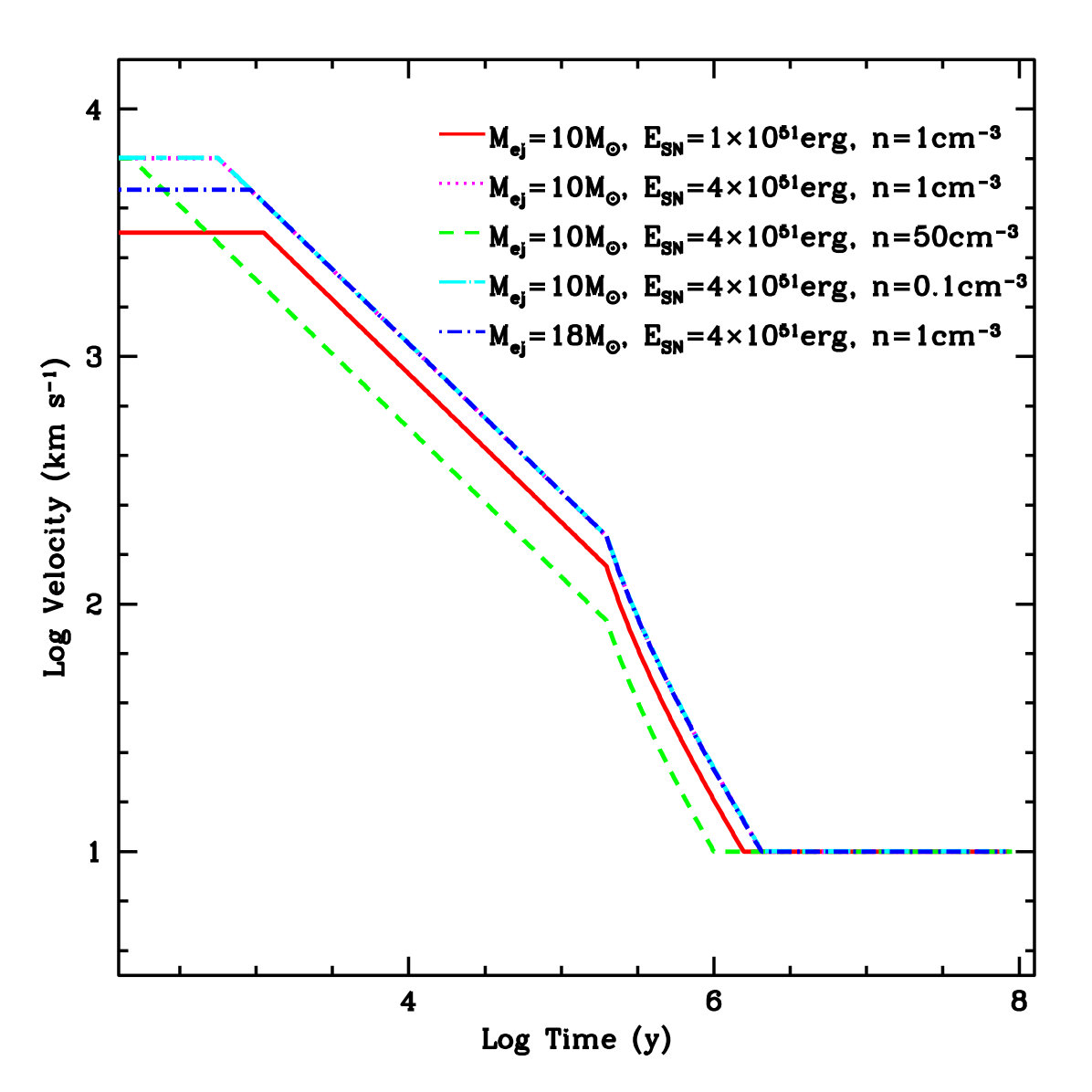 Figure 4
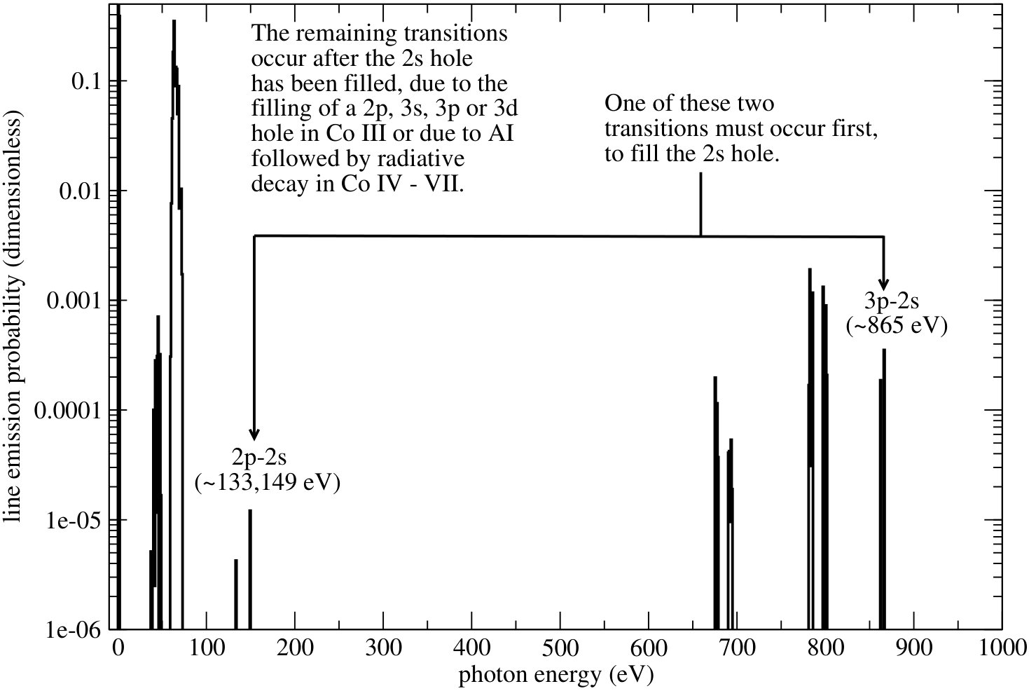 Figure 5
 Figure 6
 Figure 7
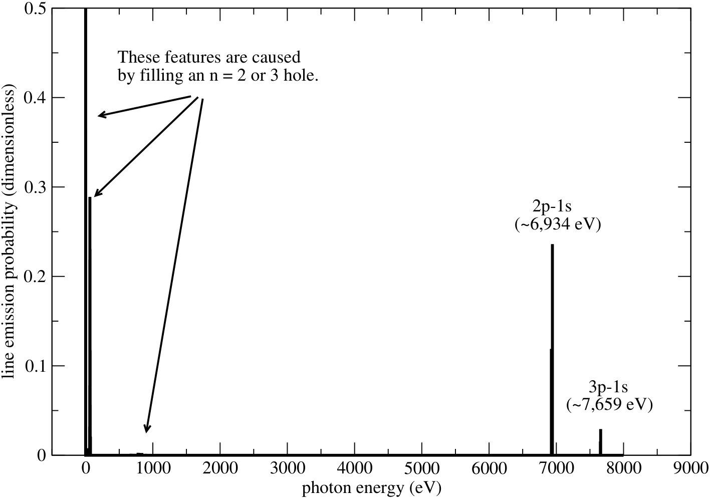 Figure 8
 Figure 9
 Figure 10
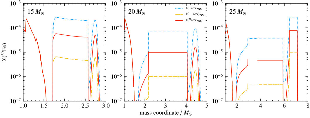 Figure 11
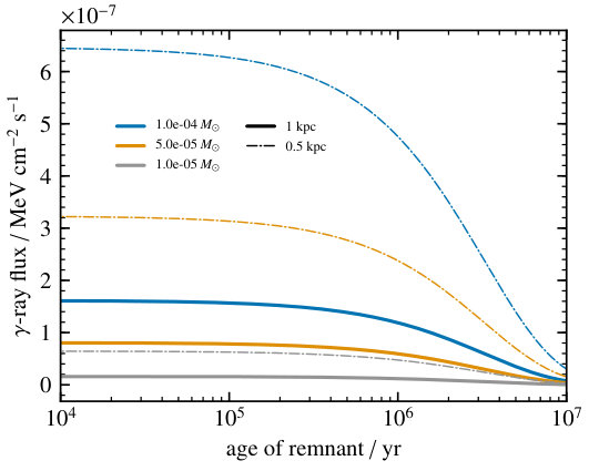 Figure 12
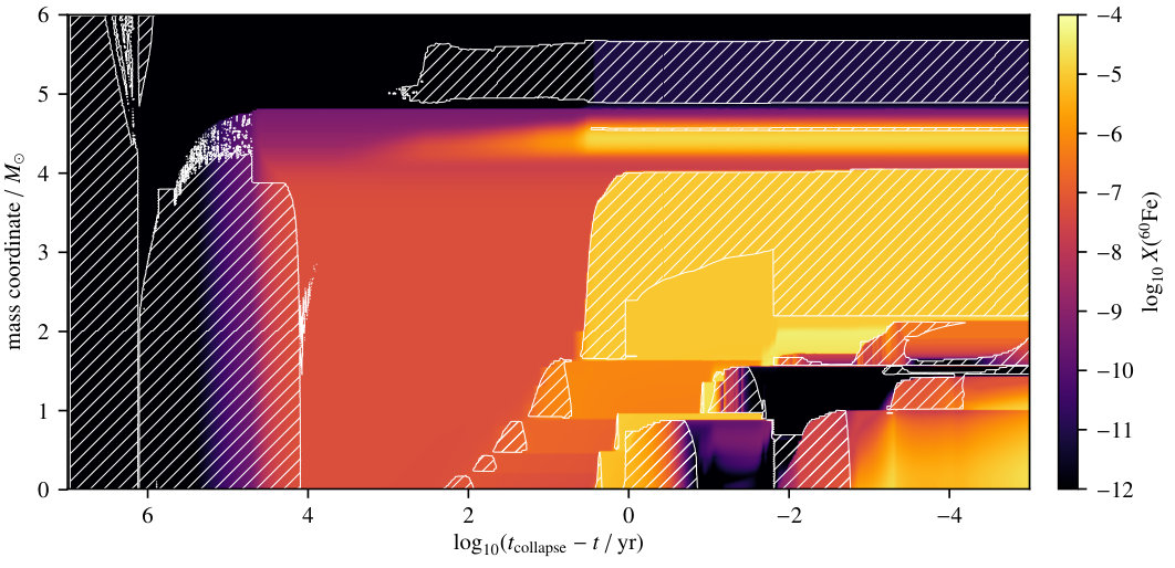 Figure 13
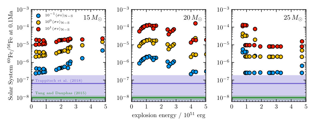 Figure 14
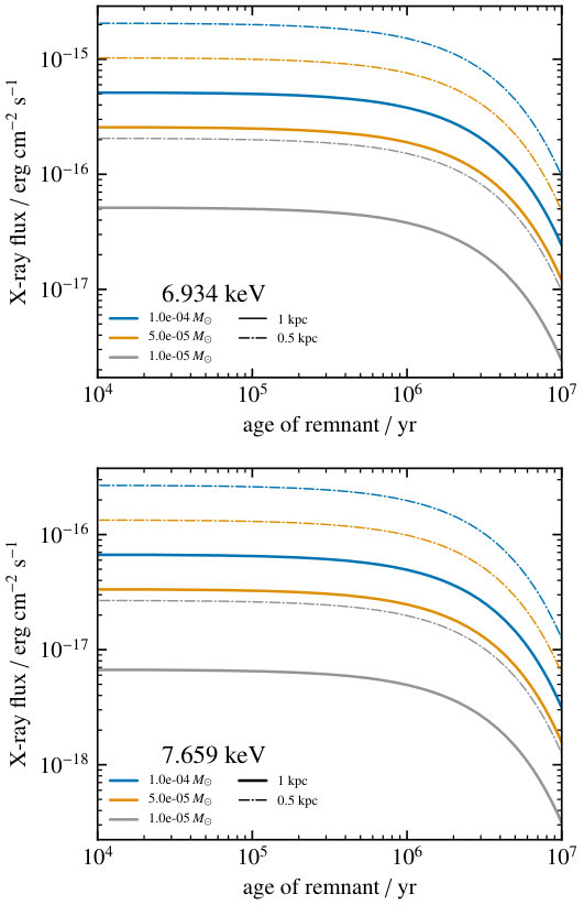 Figure 15
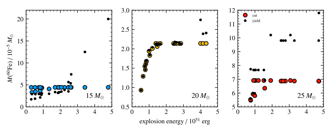 Figure 16
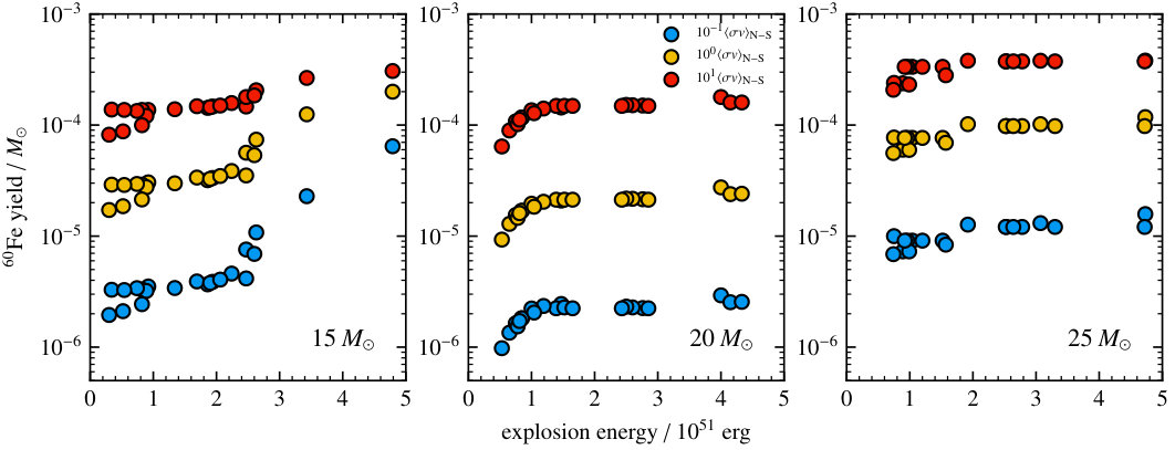 Figure 17
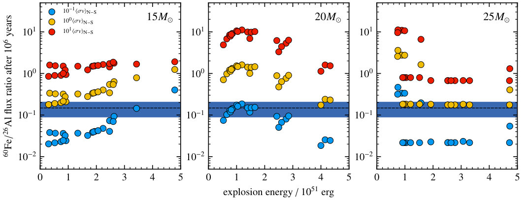 Figure 18
 Figure 19
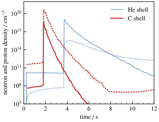 Figure 20
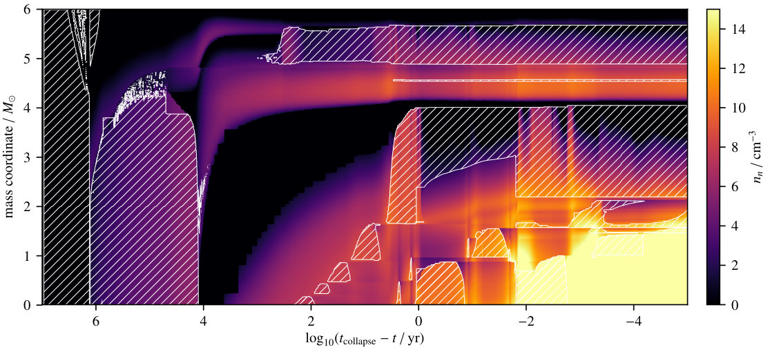 Figure 21
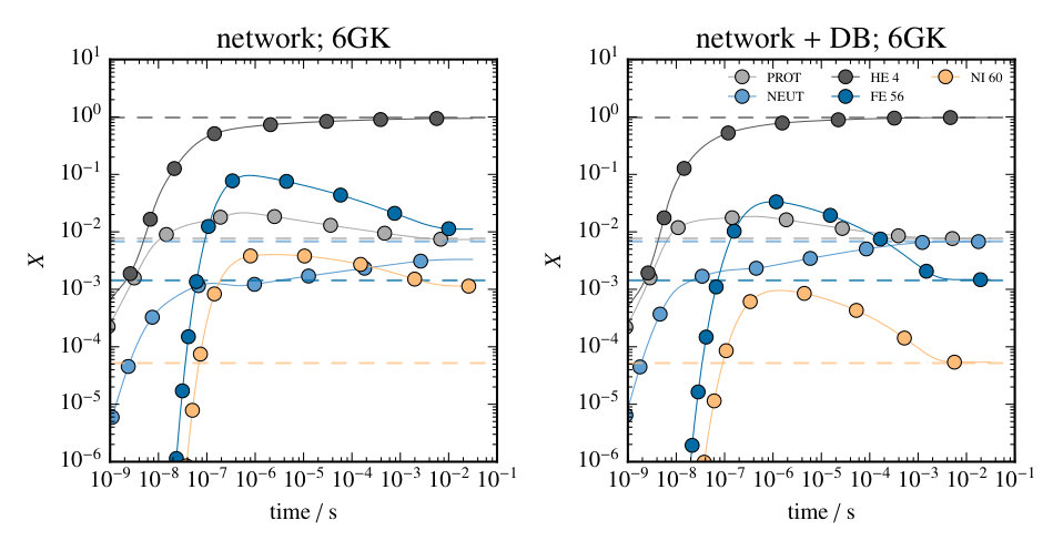 Figure 22
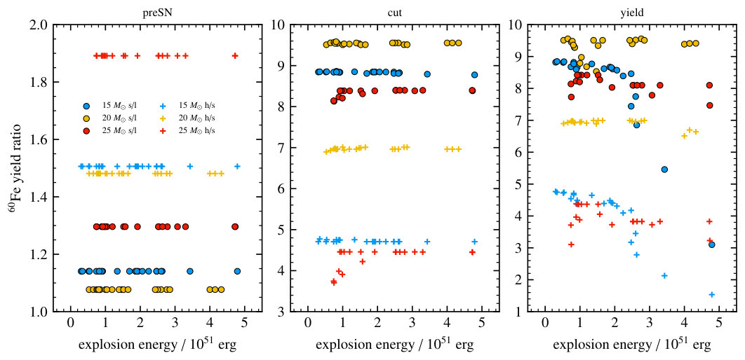 Figure 23
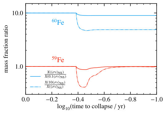 Figure 24
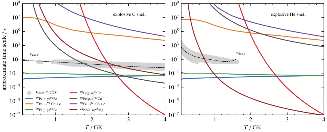 Figure 25
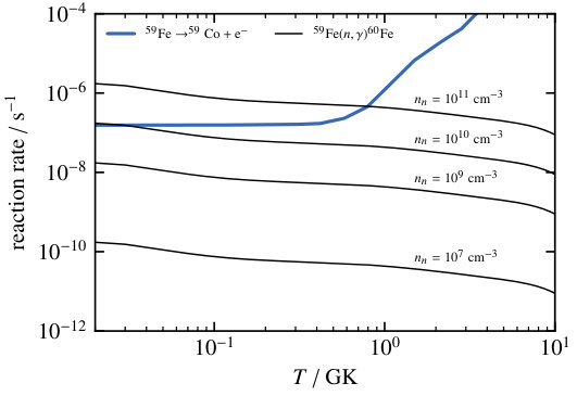 Figure 26
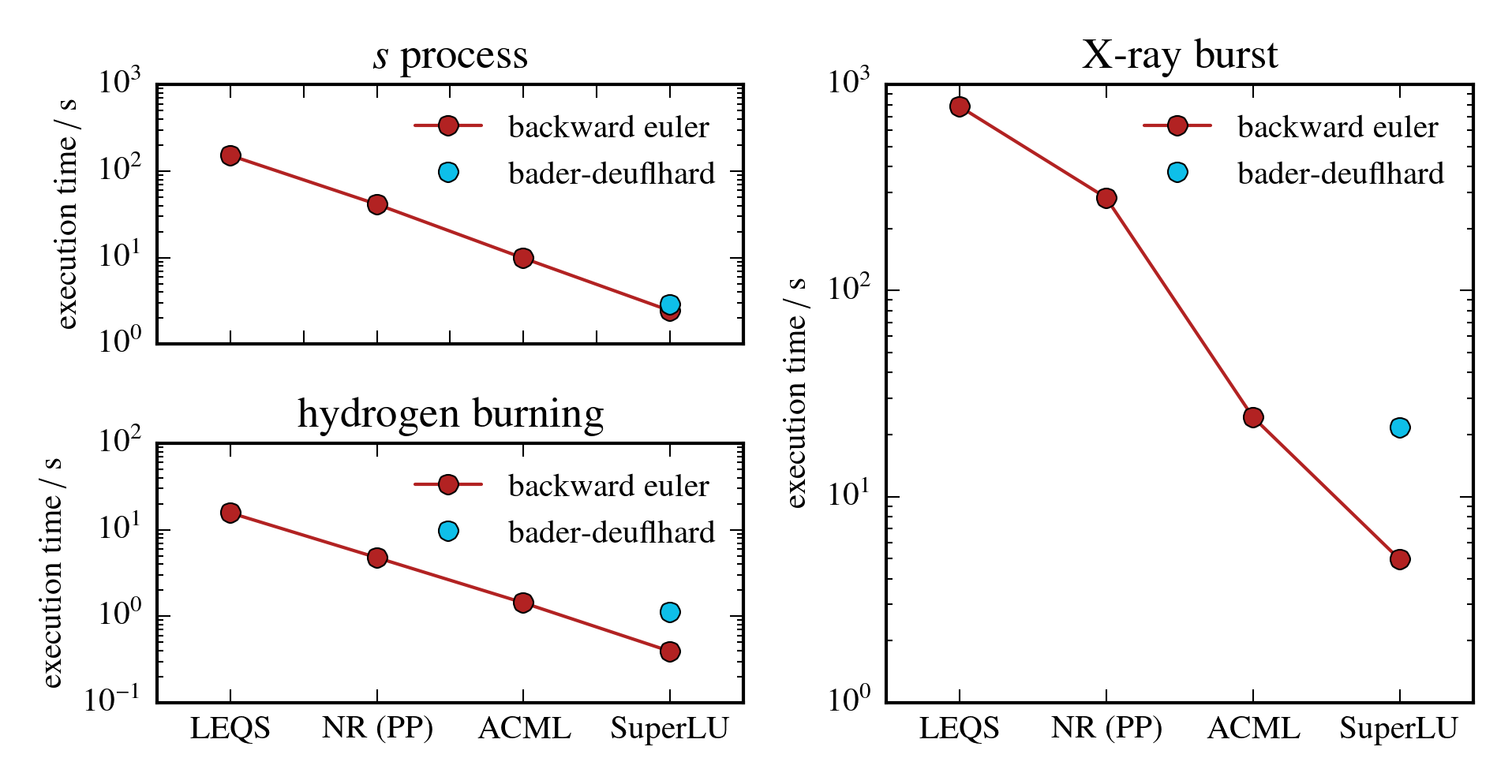 Figure 27
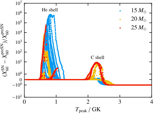 Figure 28
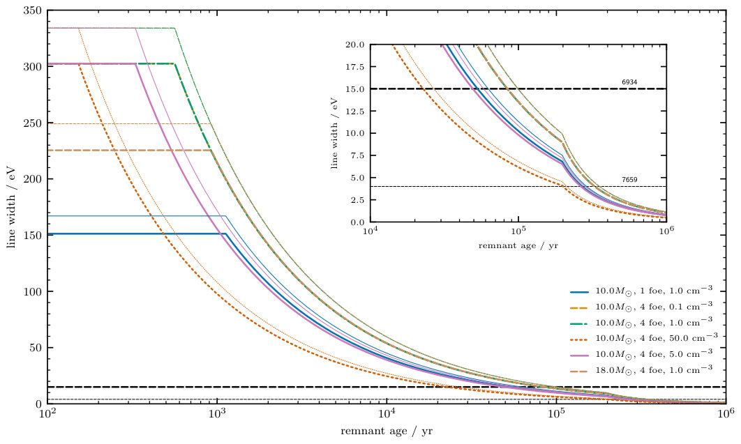 Figure 29
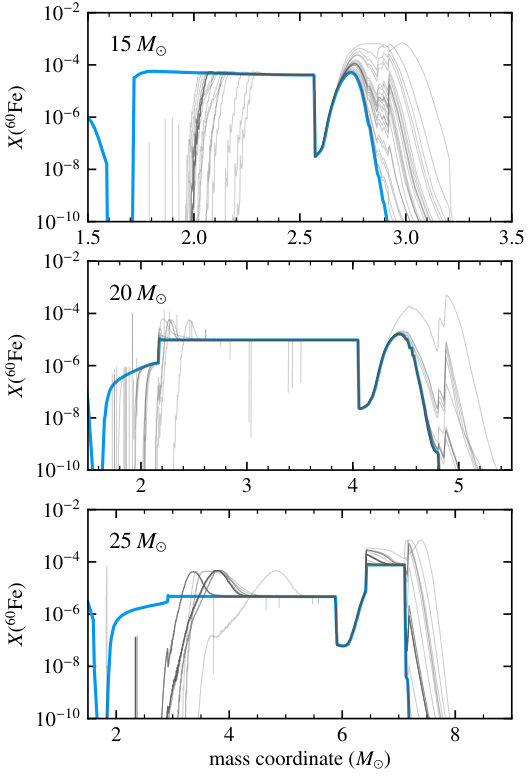 Figure 30
| pre-SN | cut | yield | pre-SN | cut | yield | pre-SN | cut | yield | yield | |||
|---|---|---|---|---|---|---|---|---|---|---|---|---|
| erg] | ||||||||||||
| 15 | 1.80 | 1.34 | 2.84 | 0.05 | 0.03 | 3.24 | 0.41 | 0.30 | 4.88 | 1.94 | 1.39 | 0.20 |
| 15 | 1.71 | 0.30 | 2.84 | 0.05 | 0.02 | 3.24 | 0.44 | 0.17 | 4.88 | 2.09 | 0.82 | 0.21 |
| 15 | 1.52 | 2.47 | 2.84 | 0.05 | 0.04 | 3.24 | 0.44 | 0.35 | 4.88 | 2.09 | 1.47 | 0.22 |
| 15 | 1.61 | 1.94 | 2.84 | 0.05 | 0.04 | 3.24 | 0.44 | 0.33 | 4.88 | 2.09 | 1.47 | 0.21 |
| 15 | 1.75 | 0.92 | 2.84 | 0.05 | 0.04 | 3.24 | 0.43 | 0.31 | 4.88 | 2.06 | 1.37 | 0.32 |
| 15 | 1.53 | 2.63 | 2.84 | 0.05 | 0.11 | 3.24 | 0.44 | 0.74 | 4.88 | 2.09 | 2.06 | 0.25 |
| 15 | 1.88 | 0.82 | 2.84 | 0.04 | 0.03 | 3.24 | 0.37 | 0.29 | 4.88 | 1.74 | 1.37 | 0.20 |
| 15 | 1.94 | 0.34 | 2.84 | 0.04 | 0.03 | 3.24 | 0.33 | 0.29 | 4.88 | 1.58 | 1.38 | 0.19 |
| 15 | 1.56 | 2.24 | 2.84 | 0.05 | 0.05 | 3.24 | 0.44 | 0.39 | 4.88 | 2.09 | 1.58 | 0.21 |
| 15 | 1.50 | 4.79 | 2.84 | 0.05 | 0.65 | 3.24 | 0.44 | 2.00 | 4.88 | 2.09 | 3.07 | 0.35 |
| 15 | 1.74 | 0.89 | 2.84 | 0.05 | 0.03 | 3.24 | 0.43 | 0.28 | 4.88 | 2.06 | 1.21 | 0.22 |
| 15 | 1.63 | 1.86 | 2.84 | 0.05 | 0.04 | 3.24 | 0.44 | 0.32 | 4.88 | 2.09 | 1.43 | 0.21 |
| 15 | 1.52 | 1.69 | 2.84 | 0.05 | 0.04 | 3.24 | 0.44 | 0.34 | 4.88 | 2.09 | 1.48 | 0.26 |
| 15 | 1.73 | 0.74 | 2.84 | 0.05 | 0.03 | 3.24 | 0.44 | 0.30 | 4.88 | 2.08 | 1.34 | 0.32 |
| 15 | 1.51 | 3.43 | 2.84 | 0.05 | 0.23 | 3.24 | 0.44 | 1.25 | 4.88 | 2.09 | 2.66 | 0.34 |
| 15 | 1.62 | 1.90 | 2.84 | 0.05 | 0.04 | 3.24 | 0.44 | 0.33 | 4.88 | 2.09 | 1.45 | 0.21 |
| 15 | 1.71 | 0.52 | 2.84 | 0.05 | 0.02 | 3.24 | 0.44 | 0.19 | 4.88 | 2.09 | 0.88 | 0.21 |
| 15 | 1.91 | 0.54 | 2.84 | 0.04 | 0.03 | 3.24 | 0.35 | 0.29 | 4.88 | 1.65 | 1.37 | 0.19 |
| 15 | 1.59 | 2.06 | 2.84 | 0.05 | 0.04 | 3.24 | 0.44 | 0.35 | 4.88 | 2.09 | 1.50 | 0.21 |
| 15 | 1.71 | 0.82 | 2.84 | 0.05 | 0.02 | 3.24 | 0.44 | 0.21 | 4.88 | 2.09 | 1.00 | 0.22 |
| 15 | 1.51 | 2.47 | 2.84 | 0.05 | 0.08 | 3.24 | 0.44 | 0.56 | 4.88 | 2.09 | 1.79 | 0.23 |
| 15 | 1.52 | 2.60 | 2.84 | 0.05 | 0.07 | 3.24 | 0.44 | 0.54 | 4.88 | 2.09 | 1.85 | 0.22 |
| 20 | 1.86 | 4.00 | 2.47 | 0.02 | 0.03 | 2.66 | 0.21 | 0.27 | 3.94 | 1.49 | 1.79 | 0.34 |
| 20 | 2.23 | 1.47 | 2.47 | 0.02 | 0.02 | 2.66 | 0.21 | 0.21 | 3.94 | 1.44 | 1.44 | 0.05 |
| 20 | 1.85 | 4.15 | 2.47 | 0.02 | 0.03 | 2.66 | 0.21 | 0.24 | 3.94 | 1.49 | 1.60 | 0.22 |
| 20 | 1.93 | 1.39 | 2.47 | 0.02 | 0.02 | 2.66 | 0.21 | 0.21 | 3.94 | 1.49 | 1.49 | 0.03 |
| 20 | 1.76 | 2.76 | 2.47 | 0.02 | 0.02 | 2.66 | 0.21 | 0.21 | 3.94 | 1.50 | 1.50 | 0.06 |
| 20 | 3.40 | 0.53 | 2.47 | 0.01 | 0.01 | 2.66 | 0.09 | 0.09 | 3.94 | 0.64 | 0.64 | 0.03 |
| 20 | 3.03 | 0.65 | 2.47 | 0.01 | 0.01 | 2.66 | 0.13 | 0.13 | 3.94 | 0.89 | 0.89 | 0.03 |
| 20 | 2.28 | 1.19 | 2.47 | 0.02 | 0.02 | 2.66 | 0.20 | 0.20 | 3.94 | 1.40 | 1.41 | 0.03 |
| 20 | 1.87 | 4.33 | 2.47 | 0.02 | 0.03 | 2.66 | 0.21 | 0.24 | 3.94 | 1.49 | 1.60 | 0.23 |
| 20 | 1.90 | 2.60 | 2.47 | 0.02 | 0.02 | 2.66 | 0.21 | 0.22 | 3.94 | 1.49 | 1.51 | 0.07 |
| 20 | 1.97 | 1.52 | 2.47 | 0.02 | 0.02 | 2.66 | 0.21 | 0.21 | 3.94 | 1.49 | 1.49 | 0.03 |
| 20 | 2.62 | 0.84 | 2.47 | 0.02 | 0.02 | 2.66 | 0.17 | 0.17 | 3.94 | 1.17 | 1.17 | 0.03 |
| 20 | 1.93 | 2.50 | 2.47 | 0.02 | 0.02 | 2.66 | 0.21 | 0.22 | 3.94 | 1.49 | 1.52 | 0.10 |
| 20 | 2.62 | 0.85 | 2.47 | 0.02 | 0.02 | 2.66 | 0.17 | 0.17 | 3.94 | 1.17 | 1.17 | 0.03 |
| 20 | 1.74 | 2.85 | 2.47 | 0.02 | 0.02 | 2.66 | 0.21 | 0.21 | 3.94 | 1.50 | 1.49 | 0.05 |
| 20 | 2.35 | 1.00 | 2.47 | 0.02 | 0.02 | 2.66 | 0.19 | 0.20 | 3.94 | 1.36 | 1.36 | 0.03 |
| 20 | 2.76 | 0.75 | 2.47 | 0.02 | 0.02 | 2.66 | 0.15 | 0.15 | 3.94 | 1.08 | 1.08 | 0.03 |
| 20 | 1.78 | 1.65 | 2.47 | 0.02 | 0.02 | 2.66 | 0.21 | 0.21 | 3.94 | 1.50 | 1.49 | 0.03 |
| 20 | 1.86 | 2.43 | 2.47 | 0.02 | 0.02 | 2.66 | 0.21 | 0.21 | 3.94 | 1.49 | 1.49 | 0.05 |
| 20 | 2.85 | 0.78 | 2.47 | 0.02 | 0.02 | 2.66 | 0.15 | 0.15 | 3.94 | 1.02 | 1.02 | 0.03 |
| 20 | 2.70 | 0.81 | 2.47 | 0.02 | 0.02 | 2.66 | 0.16 | 0.16 | 3.94 | 1.12 | 1.12 | 0.03 |
| 20 | 2.47 | 1.04 | 2.47 | 0.02 | 0.02 | 2.66 | 0.18 | 0.18 | 3.94 | 1.27 | 1.28 | 0.03 |
| 25 | 1.84 | 1.04 | 2.06 | 0.08 | 0.09 | 2.67 | 0.69 | 0.77 | 5.05 | 3.08 | 3.35 | 0.91 |
| 25 | 1.83 | 3.07 | 2.06 | 0.08 | 0.13 | 2.67 | 0.69 | 1.02 | 5.05 | 3.08 | 3.80 | 1.22 |
| 25 | 2.38 | 4.73 | 2.06 | 0.08 | 0.16 | 2.67 | 0.69 | 1.18 | 5.05 | 3.05 | 3.81 | 0.63 |
| 25 | 4.66 | 0.89 | 2.06 | 0.07 | 0.07 | 2.67 | 0.59 | 0.60 | 5.05 | 2.36 | 2.38 | 0.05 |
| 25 | 1.83 | 1.52 | 2.06 | 0.08 | 0.09 | 2.67 | 0.69 | 0.77 | 5.05 | 3.08 | 3.35 | 0.91 |
| 25 | 1.83 | 0.96 | 2.06 | 0.08 | 0.09 | 2.67 | 0.69 | 0.77 | 5.05 | 3.08 | 3.35 | 0.91 |
| 25 | 3.13 | 1.92 | 2.06 | 0.08 | 0.13 | 2.67 | 0.69 | 1.02 | 5.05 | 3.08 | 3.80 | 1.22 |
| 25 | 2.35 | 2.53 | 2.06 | 0.08 | 0.12 | 2.67 | 0.69 | 0.98 | 5.05 | 3.06 | 3.75 | 1.21 |
| 25 | 2.35 | 4.72 | 2.06 | 0.08 | 0.12 | 2.67 | 0.69 | 0.98 | 5.05 | 3.06 | 3.75 | 1.21 |
| 25 | 2.35 | 2.78 | 2.06 | 0.08 | 0.12 | 2.67 | 0.69 | 0.98 | 5.05 | 3.06 | 3.75 | 1.21 |
| 25 | 5.60 | 0.75 | 2.06 | 0.07 | 0.10 | 2.67 | 0.55 | 0.77 | 5.05 | 2.03 | 2.40 | 0.05 |
| 25 | 2.35 | 3.30 | 2.06 | 0.08 | 0.12 | 2.67 | 0.69 | 0.98 | 5.05 | 3.06 | 3.75 | 1.21 |
| 25 | 4.89 | 0.99 | 2.06 | 0.07 | 0.07 | 2.67 | 0.58 | 0.60 | 5.05 | 2.27 | 2.32 | 0.05 |
| 25 | 3.73 | 1.57 | 2.06 | 0.08 | 0.08 | 2.67 | 0.64 | 0.69 | 5.05 | 2.68 | 2.81 | 0.09 |
| 25 | 1.84 | 1.20 | 2.06 | 0.08 | 0.09 | 2.67 | 0.69 | 0.77 | 5.05 | 3.08 | 3.35 | 0.91 |
| 25 | 5.47 | 0.74 | 2.06 | 0.07 | 0.07 | 2.67 | 0.55 | 0.56 | 5.05 | 2.07 | 2.08 | 0.05 |
| 25 | 2.34 | 2.52 | 2.06 | 0.08 | 0.12 | 2.67 | 0.69 | 0.98 | 5.05 | 3.06 | 3.75 | 1.21 |
| 25 | 1.84 | 0.92 | 2.06 | 0.08 | 0.09 | 2.67 | 0.69 | 0.77 | 5.05 | 3.08 | 3.35 | 0.91 |
| 25 | 2.35 | 2.64 | 2.06 | 0.08 | 0.12 | 2.67 | 0.69 | 0.98 | 5.05 | 3.06 | 3.75 | 1.21 |
Peer Reviews
No public reviews on file for this paper yet. If you reviewed it on a platform where reviews are public (OpenReview, ICLR, NeurIPS, ICML), you can paste yours below so the community can read it here.
Videos
No videos yet. Explain this paper in a talk, walkthrough, or lecture? Add one.
60Fe in core-collapse supernovae and
prospects for X-ray and -ray detection in supernova remnants
Samuel W. Jones1,2,†,, Heiko Möller2,3,4,†, Chris L. Fryer2,†, Christopher J. Fontes1, Reto Trappitsch5,†, Wesley P. Even2,†, Aaron Couture6,†, Matthew R. Mumpower7, and Samar Safi-Harb8
1X Computational Physics (XCP) Division, Los Alamos National Laboratory, New Mexico 87545, USA
2Computer, Computational and Statistical Sciences (CCS) Division, Los Alamos National Laboratory, New Mexico 87545, USA
3Institut für Kernphysik (Theoriezentrum), Technische Universität Darmstadt, Schlossgartenstraße 2, 64289 Darmstadt, Germany
4GSI Helmholtzzentrum für Schwerioneneforschung, Planckstraße 1, 64291 Darmstadt, Germany
5Nuclear and Chemical Sciences Division, Lawrence Livermore National Laboratory, Livermore, CA 94550, USA
6Physics Division, Los Alamos National Laboratory, New Mexico 87545, USA
7Theoretical Division, Los Alamos National Laboratory, New Mexico 87545, USA
8Department of Physics and Astronomy, University of Manitoba, Winnipeg, MB R3T 2N2, Canada
† NuGrid Collaboration E-mail: [email protected]
(Accepted 15 February 2019. Received 10 December 2018)
Abstract
We investigate in massive stars and core-collapse supernovae focussing on uncertainties that influence its production in 15, 20 and 25 stars at solar metallicity. We find that the yield is a monotonic increasing function of the uncertain cross section and that a factor of 10 reduction in the reaction rate results in a factor 8–10 reduction in the yield; while a factor of 10 increase in the rate increases the yield by a factor 4–7. We find that none of the 189 simulations we have performed are consistent with a core-collapse supernova triggering the formation of the Solar System, and that only models using cross section that is less than or equal to that from NON-SMOKER can reproduce the observed / line flux ratio in the diffuse ISM. We examine the prospects of detecting old core-collapse supernova remnants (SNRs) in the Milky Way from their -ray emission from the decay of , finding that the next generation of gamma-ray missions could be able to discover up to such old SNRs as well as measure the yields of a handful of known Galactic SNRs. We also predict the X-ray spectrum that is produced by atomic transitions in following its ionization by internal conversion and give theoretical X-ray line fluxes as a function of remnant age as well as the Doppler and fine-structure line broadening effects. The X-ray emission presents an interesting prospect for addressing the missing SNR problem with future X-ray missions.
keywords:
nuclear reactions, nucleosynthesis, abundances – stars: abundances, massive – supernovae: general – gamma-rays: stars
††pubyear: 2019††pagerange: 60Fe in core-collapse supernovae and prospects for X-ray and -ray detection in supernova remnants–60Fe in core-collapse supernovae and prospects for X-ray and -ray detection in supernova remnants
1 Introduction
Gamma-ray detections of nuclear decay lines in the Galaxy from either point or diffuse sources provide an opportunity to test stellar evolution theory (see, e.g. Diehl, 2013, and references therein for a review centered around the INTEGRAL mission). Short-lived radioactive (SR or SLR)111 There are conflicting definitions of what constitutes a short-lived radionuclide (SR or SLR) in the literature, but broadly speaking they are nuclides with half-lives on the order of a million years or less (some definitions extend up to half-lives of 50 million years). The same isotopes have also been labeled long-lived radioactive isotopes in relevant works. isotopes synthesized in and ejected from stars contribute a portion of the diffuse Galactic gamma-ray foreground in the Milky Way. In particular, decay lines from the radionuclides 26Al and , with half lives of yr and yr, respectively, have been measured by multiple instruments, most recently by the INTEGRAL/SPI mission (Smith, 2004; Wang et al., 2007; Bouchet et al., 2011).
Although it is not naturally occurring, terrestrial deposits of live have in fact been detected in layers of sea-floor sediment on Earth (Knie et al., 1999, 2004; Wallner et al., 2016, see also Fitoussi et al., 2008) and must have accreted from outside of the Solar System. The most recent measurements have identified two such accretion events yr and yr ago (Wallner et al., 2016), consistent with the origin being ejecta from supernovae approximately pc from Earth (Fields et al., 2005). The Upper Centaurus Lupus and Lower Centaurus Crux stellar subgroups have been kinematically identified as having passed through the region currently occupied by the Local Bubble222the Local Bubble is a cavity in the ISM that contains the Solar System (LB) yr ago (Fuchs et al., 2006). Supernovae exploding in those subgroups would consistently explain both the origin of the LB and the terrestrial deposits of (Feige, 2014; Schulreich et al., 2017).
The ratio of gamma-ray fluxes from and in the interstellar medium (ISM) is of particular significance. This value, since the first measurements from HEAO-3 (Mahoney et al., 1982), has stayed in the range (see Wang et al., 2007, their Figure 7 and Table 2). Bouchet et al. (2011), performing new analysis of the SPI/INTEGRAL data in 2011, found a flux ratio of (cf. Wang et al.’s ). Recent measurements (Feige et al., 2018) further determined a lower limit for the / ratio in the local interstellar medium of by analyzing these SLRs in deep-sea sediments. This measurement agrees well with gamma-ray flux measurements. These values present a constraint or calibration point for stellar evolution theory. That is, massive stars are thought to produce the bulk of the and in the Galaxy and therefore, if accurate, models of massive stars should be able to reproduce the observed ratio (Timmes et al., 1995; Rauscher et al., 2002; Limongi & Chieffi, 2003, 2006).
Timmes et al. (1995) present galactic chemical evolution (GCE) simulations for and in the Milky Way. Remarkably, the flux ratio their models predicted was 0.16 – a near-perfect match to the observational measurements. Newer stellar evolution and explosion calculations (Rauscher & Thielemann, 2000; Limongi & Chieffi, 2003) predicted ratios further from the measured value ( and , respectively; see Prantzos, 2004, their Figure 2). A few years later, Limongi & Chieffi (2006) published a set of models that were able to reproduce the observed flux ratio when adopting the mass loss rates of Langer (1989) as opposed to those published a decade later by Nugis & Lamers (2000) for the Wolf-Rayet phase.
The massive star and core-collapse supernova (CCSN) models used by Timmes et al. (1995) were from Woosley & Weaver (1995) and used the cross section from Woosley et al. (1978). The Rauscher et al. (2002) models used the cross section from Rauscher & Thielemann (2000). While both cross sections originated from Hauser-Feshbach calculations there were still differences (Woosley et al., 2003). This could explain at least part of the discrepancy between the / flux ratios predicted by Timmes et al. (1995) and Rauscher et al. (2002). We note at this point that in both examples given here (winds and cross section), adopting more modern physics has exacerbated the tension between models and observations.
Tur et al. (2010) showed that the yields of radioactive and in massive stars and CCSNe are sensitive to the and particularly the 12CO He-burning reaction rates. Varying these reaction rates by up to twice the experimental uncertainty resulted in up to a factor of five change in the ejected mass of and a factor of 10 change in the / yield ratio. Some of the more drastic alterations to the amount of inside a massive star come from structural changes such as the size of a convective region or the occurrence or not of convective shell mergers (Rauscher et al., 2002; Ritter et al., 2018). Substantial structural changes can be triggered by seemingly small changes to the reaction rates (Tur et al., 2010), illustrating the cumulative effect of the prevalent uncertainties in stellar evolution modelling such as rotation (Palacios et al., 2005; Edelmann et al., 2017), convection and convective boundaries (e.g. Meakin & Arnett, 2007; Jones et al., 2017; Davis et al., 2018), mass loss (Palacios et al., 2005; Limongi & Chieffi, 2006; Renzo et al., 2017), and opacities (Woosley & Heger, 2007a).
There are other astrophysical sites that have been proposed as candidates in which and could be produced in significant quantities that we mention here for completeness. For example, can be made in super-AGB stars (Lugaro et al., 2012) and high-density type-Ia supernovae that include a deflagration phase (Woosley, 1997). Electron-capture supernovae (ECSNe) have also been proposed to contribute at least of the live in the Galaxy (Wanajo et al., 2013), although the progenitor scenario remains rather uncertain with respect to the fraction of stars that explode as ECSNe (Doherty et al., 2017). The nucleosynthesis is likely similar in the lowest-mass CCSNe, however (Wanajo et al., 2018). It is still an open question as to whether ECSNe are indeed core-collapse supernovae (Jones et al., 2016), and in the case that they are thermonuclear explosions they would exhibit very large yields and / ratios (Jones et al., 2018).
Our work is also motivated by addressing the missing SNR problem. Radio and high-energy observations of SNRs reveal nearly 400 SNRs in our Galaxy (Green, 2017; Ferrand & Safi-Harb, 2012). However, at a Galactic supernova frequency of one event every 30–50 years (Tammann et al., 1994), and the lifetime of an SNR being 106 years, the total number of SNRs should be at least an order of magnitude higher than observed. This missing SNR problem can be at least partly attributed to a selection effect against the old, low-surface brightness SNRs. We suggest the decay of 60Fe as a means to detect SNRs at very late times.
In this paper we focus on two relatively unexplored – but known – uncertainties in the production of in CCSN models. The first is the cross section for which there are still no direct measurements available (see Woosley et al., 2003). The second is the way in which the 1D CCSN simulations are performed, how they are parameterized and with what parameter choices. A third relevant uncertainty but one that we do not address in this work is the dependence on the dimensionality of the CCSN simulation.
2 Methodology and Simulations
We present spherically symmetric (1D) stellar evolution (SE) and CCSN simulations with emphasis on their nucleosynthesis, which is calculated in post-processing. We used three different reaction cross sections for the nucleosynthesis covering a range of two orders of magnitude.
2.1 Stellar evolution models
Stellar evolution models were computed using the KEPLER code (Weaver et al., 1978; Rauscher et al., 2002; Woosley & Heger, 2007b), ending when the collapsing iron core achieves an infall velocity of 1000 km s*-1*. We computed models with initial masses of 15, 20 and 25 , all with initial metallicity and relative fractions of the metals after Grevesse & Noels (1993). The modelling assumptions made for these simulations were the same as for the KEPLER models by Jones et al. (2015) but with different rates for three of the key reactions responsible for energy generation during H and He burning. The 14NO reaction rate is now taken from Imbriani et al. (2004), the triple- reaction rate is from Fynbo et al. (2005), and the 12CO reaction rate is taken from Kunz et al. (2002). Jones et al. (2015) have presented a relatively detailed description of the methodology including a comparison with two other stellar evolution codes.
2.2 Core-collapse supernova simulations
The CCSN models used for this work are a suite of parameterized simulations by Fryer et al. (2018) which used the 1D Lagrangian hydrodynamics supernova code described in Herant et al. (1994) and Fryer et al. (1999) with initial conditions provided by the collapsing KEPLER models. The parameterization of the 1D explosions is designed to mimic the 3D convection engine first demonstrated by Herant et al. (1994). Indeed, except for low-mass progenitors, 1D models typically do not self-consistently produce supernova explosions owing to the lack of convective energy transport. Uncertainties in the multi-dimensional simulations of the convective engine allow for a range of results and we use parameterized models to give us a flavor of the possible explosion conditions. Energy is injected above the proto-neutron star over different spatial extents to mimic the size of the convective region and at different durations to mimic the timescale of the engine (for details see Fryer et al., 2018). In total there are 63 CCSN simulations of the 3 progenitors that we consider for this work. We note that a shortcoming of our approach is that neutrino interactions are omitted, which are known to substantially modify the electron fraction of the material above the proto-neutron star in the NSE region (e.g. Qian & Woosley, 1996; Fröhlich et al., 2006; Rampp & Janka, 2000) and can also modify the composition of the ejecta via -spallation processes. This should not be a serious concern for the present work, because the production/destruction of is not influenced by neutrino interactions, however Timmes et al. (1995) have shown the the yield can be increased by up to about 50 per cent when -spallation reactions are included in simulations.
2.3 Post-processing nucleosynthesis code
The nucleosynthesis calculations were performed using a derivative of the NuGrid nuclear reaction network code (see, e.g., Pignatari et al., 2016; Ritter et al., 2017).
The SE calculations were post-processed using the code MPPNP333Multi-zone Post-Processing Network – Parallel, which evolves the composition forwards in time for every computational grid cell over one stellar evolution time step and subsequently performs a mixing step over the whole model with a time-implicit diffusion solve de-coupled from the network integration using a diffusion coefficient from the stellar evolution code. The reaction network for the evolution up to the pre-supernova stage included a pool of about isotopes and about reactions.
For the supernova simulations, we used the code TPPNP444Tracer particle Post-Processing Network – Parallel, which is simply a different program for handling the I/O for tracer particles (as opposed to spherically symmetric stellar models) and capitalising on the embarassingly parallel nature of post-processing Lagrangian particles between which we assume there to be no mixing. Since our CCSN simulations were performed with a 1D Lagrangian hydrodynamics code (see Section 2.2) without adaptive mesh refinement, the evolution of the composition for each grid cell can be considered to be mutually exclusive from that in all the other grid cells. The reaction network for the explosions was substantially larger than for the stellar evolution models (in fact, probably larger than necessary), with approximately 5000 isotopes and 67000 reactions.
Both programs MPPNP and TPPNP use the same underlying physics and solver libraries, to which several additions were made during the course of this work that we feel are worthy of mention here. They are:
- •
a semi-implicit extrapolation time integrator (so-called Bader-Deuflhard or generalised Bulirsch-Stöer method; Bader & Deuflhard, 1983; Deuflhard, 1983, but see also Timmes, 1999),
- •
a Cash-Karp Runge-Kutta integration for the coupling of weak reactions with the NSE state,
- •
calculation of reverse reaction rates using the principle of detailed balance555see the appendix of Calder et al. (2007) for a concise formulation including plasma Coulomb corrections,
- •
integration of SuperLU sparse matrix solver library for solving the linear system (Demmel et al., 1999; Li et al., 1999; Li, 2005), and
- •
implementation of electron screening corrections from Chugunov et al. (2007).
A discussion of these few additions is deferred to Appendix A.1.
Reaction rates from JINA Reaclib (Cyburt et al., 2010), KaDoNiS (Dillmann et al., 2006), NACRE (Angulo et al., 1999) and NON-SMOKER (Rauscher & Thielemann, 2000), as well as from Fuller et al. (1985), Takahashi & Yokoi (1987), Goriely (1999), Langanke & Martínez-Pinedo (2000), Iliadis et al. (2001) and Oda et al. (1994) were used. Of particular relevance for this work is that the reaction rate used was the JINA Reaclib fit to the reaction rate from Rauscher & Thielemann (2000). We used the KaDoNiS reaction rates for the 58Fe and 60Fe reactions, taking the v0.3 values where available. For the reaction we use the recommended rate from Jaeger et al. (2001). The reaction rate is from Langanke & Martínez-Pinedo (2000).
3 The cross section
In astrophysical scenarios, the primary reaction mechanism to produce 60Fe is through . Unfortunately, this reaction is very difficult to measure directly. 59Fe has a short half-life of 44.5 days and emits gamma-rays with energies in excess of 1 MeV. The gold-standard for neutron capture measurements is the differential time-of-flight (TOF) measurement technique. This requires a sample of the isotope of interest to be produced and placed inside of a detector array. Past studies (Couture & Reifarth, 2007) showed that current and planned neutron experimental facilities have 2-4 orders of magnitude too few neutrons to perform a TOF measurement on 59Fe. An indirect Coulomb-dissociation measurement by Uberseder et al. (2014) places constraints on the gamma-ray strength function used in the statistical cross-section calculation, however, this measurement was only sensitive to components. There is growing evidence that the component, not accessible in the Uberseder measurement, play an important role in neutron capture cross sections (Larsen & Goriely, 2010; Mumpower et al., 2017). Finally, neutron capture cross sections on isotopes near shell closures, such as 59Fe, are notoriously difficult to predict because individual neutron resonances can dominate the nuclear reaction rate. As a result, we have chosen to perform these studies with a cross-section ranging up and down a factor of ten from the standard nonsmoker rates. This is consistent with standard variations for neutron capture for unstable isotopes (Mumpower et al., 2012, 2016).
4 Nucleosynthesis results
In this section, we present the results of the nucleosynthesis calculations as they pertain to the production of radioactive . We briefly review the production of in massive stars via the weak s-process, following which we present an analysis of the contribution of shock heating in the CCSN to the synthesis of . Lastly, we assess the impact of varying the cross section on the amount of produced.
4.1 in massive stars
The stellar models initially contain no , owing to our adoption of the Solar distribution of the metals (Grevesse & Noels, 1993) and having a comparatively short half life. is predominantly a product of the weak s-process and is produced by successive neutron captures beginning from seed nuclei from the gas cloud that collapsed to form the star. The reaction is the source of the neutrons. is therefore considered to be a secondary isotope. The reaction sequence takes place very slowly in the convective He-burning core towards the end of core He-burning, but much faster in the C-burning and Ne-burning shells, and in the hotter, deeper portion of the He-burning shell later in the star’s life. The bulk of the produced via the weak s-process is made in the He-, C-, and and Ne-burning shells where the temperatures are high enough for the reaction to be sufficiently activated that the neutron density is high enough for the reaction to compete with the -decay of . This requires neutron densities of cm*-3*, as is illustrated in Figure 1 (see also Limongi & Chieffi, 2006).
At temperatures in excess of about 2 GK, is destroyed by , and reactions and therefore the production is most vigorous in the Ne-burning shells, which approach the maximum temperature for its production and above which it would be destroyed. Indeed, O burning proceeds Ne burning and usually engulfs the entire portion of the star in which Ne burning operated, raising the temperature above the destruction threshold. Figure 2 shows a map of the mass fraction of in the core of the star throughout its entire life (top panel) along with the neutron density (bottom panel). The cross-hatched regions are convectively unstable. The production of is clearly correlated with higher neutron densities. It is also produced in the iron core during Si-burning and persists in the central region of the star until the star explodes. This can be seen in the top panel of Figure 2, onwards from in the central 1.5 of the star. However, this material will likely not escape the gravitational potential in the collapsing core and will instead become part of the compact remnant, therefore not contributing to the final yield at all. In fact, this is the case in all of the CCSN simulations presented in this work (see Section 4.2).
The evolution of in a massive star culminates at the pre-supernova stage where the bulk of is contained in the Fe core, the Si-burning shell, C-burning shell and in the deeper – and often convectively stable – portion of the He-burning shell (see Figure 3). The amount of in the C-burning and He-burning shells is shown to be sensitive to the uncertain reaction cross section but we defer the discussion of this sensitivity to Section 4.3.
4.2 in CCSNe
There are two key factors affecting the final yield of from CCSNe once the amount in the star at the pre-supernova stage is known. These are (i) which material becomes gravitationally unbound and which remains bound to become the proto-neutron star (i.e. where is the mass cut) and (ii) heating in the post-bounce shock wave and cooling during the expansion following the passage of the shock.
In order to separate out these two effects, in Figure 4 we show the total mass of in the star at the pre-supernova stage minus what goes into the compact remnant (“cut", filled circles) and the final yield, which includes the effect of shock heating on the unbound material (“yield", black dots). These quantities are plotted as a function of asymptotic kinetic explosion energy. While a substantial amount of is always lost to the compact remnant, there is a significant contribution from the shock heating in most of the 15 and 25 models, but not so much in the 20 models. In general the net effect of the shock-heating on the 15 models is to destroy rather than create it, with the exception of the 5 most energetic explosions. Conversely, the general net effect of the shock heating in the 25 models is to produce more , with the largest impact again for the most energetic explosions. Now that we have an idea of the net effects of the s-process, mass cut and the shock heating on the final ejected mass of , we will present a more detailed view of what is happening to the in the explosion.
The final abundance profiles of for all of our simulations is shown in Figure 5 together with the pre-supernova abundance profile. This figure serves as a reference point for the following discussion.
An overview of the shock nucleosynthesis is given in Figure 6, which shows the ratio of final to initial in the supernova as a function of peak temperature. Two distinct peaks are seen and correspond to the conditions met during explosive He and C shell burning. Additionally there is a deficit in at high peak temperatures. The details of the processes taking place are given in the remainder of this section.
Firstly, the shock wave compresses and heats the inner portion of the star, and sometimes also the lower section of the C shell into NSE. The electron fractions are close to but slightly below 0.5, favoring nuclei with . Much lower electron fractions would be needed in order for to be abundant in this scenario: . Therefore, in the deepest parts of the supernova ejecta virtually all of the is destroyed by the readjustment of the composition to its statistical equilibrium. The electron fraction does not change appreciably during the passage of the shock in this region because the time scales of the weak rates at those densities are much longer than the post-shock expansion time scale of the ejecta. Therefore, it is generally not possible to obtain a low enough to favour production in these deeper layers of the star during the explosion. Indeed, even near the proto-neutron star surface where electron capture can neutronize the ejecta, neutrino interactions prevent the electron fraction from becoming this low (e.g. Qian & Woosley, 1996; Fröhlich et al., 2006; Rampp & Janka, 2000).
As the shock propagates through the C shell and the peak temperature in the shocked material decreases, the material is no longer heated as far as NSE but is still destroyed by , and where the peak temperature exceeds approximately 3 GK. This is illustrated in Figure 7, in which the left panel shows time scales of several key reactions taking place during explosive C shell burning, comparing them to the post-shock expansion time scale , which is the e-folding time of the post-shock temperature (Fryer et al., 2018). Above 3 GK, the , and reactions are operating on time scales faster than or comparable to the reaction that is creating . Below about 2 GK, the fastest reaction is , however the neutron source reaction becomes much slower than the post-shock expansion time scale, so although the thermodynamic conditions and the composition are optimal for production, the whole process operates on too short a time scale to be relevant during the explosion. Between 2 and 3 GK, however, there is a sweet spot where is the fastest reaction, and the destructive reactions have a time scale similar to or less than . Between 2 GK and 3 GK the reaction still has a time scale that is comparable to , and therefore neutrons will be released, achieving neutron densities of cm*-3* (see Figure 8) which are sufficient to overcome the enhancement in -decay rates of 59Fe . The increase in time scale of the reaction below about 2 GK is the main reason why there is no created in the outer portion of the C shell (see Figure 5).
The neutron densities reached in explosive He shell burning when the shock reaches the He shell are very similar to those attained in explosive C shell burning (see Figure 8). While the peak temperature of the shock is lower ( GK) the abundance is much higher: compared to in the C shell. The He abundance is also much higher in the He shell, as one might exepect. The time scale of neutron release via is again faster than or comparable to the post-shock expansion time scale (Figure 7, right panel) because the proton densities are so much lower than in the C shell (Figure 8), there is no significant destruction of by reactions. Moreover, because the peak temperature is lower, there is also no discernible destruction of by reactions either.
Again, the total final yield is a monotonic increasing function of the reaction rate. The impact of modifying the reaction rate from NON-SMOKER through both the stellar evolution and the explosion is shown in Figure 9. A discussion of the impact of the cross section on the production of is presented in Section 4.3.
4.3 Impact of the cross section and total uncertainty
In Figure 9 we have shown that the total ejected mass of is sensitive to and is a monotonic increasing function of the cross section. The yield appears to scale almost linearly with the cross section, suggesting that if the uncertainty in the cross section spans two orders of magnitude, then the uncertainty in the yield also spans approximately two orders of magnitude. In this short section we will examine the sensitivity of the mass of in a massive star to the cross section at the pre-supernova stage and in the supernova ejecta in a little more detail.
All of the stellar evolution and supernova nucleosynthesis post-processing calculations were performed three times: with the cross section from NON-SMOKER (Rauscher & Thielemann, 2000) and with cross sections ten times lower and ten times higher (s, l and h; standard, low, high, respectively). To get an insight into the impact of varying the cross section on the production of , we look at the masses of in the simulations with different cross sections relative to one another. More specifically, we have looked at the ratios and , where the subscript denotes the cross section that was used. Three different masses were used in order to separate out the different processes affecting the production of : the total mass of in the star at the presupernova stage including the material that will form the neutron star (preSN), the total mass of in the star at the presupenova stage excluding the material that will form the neutron star (cut), and the total ejected mass of in the supernova explosion after shock heating (yield). This information is presented in the top three panels of Figure 10.
Increasing or depressing the cross section by a factor of 10 results in at most a factor of 2 change in the mass of in the star at the presupernova stage. This is because a large fraction has been produced in the iron core where the material is either in NSE or close to NSE. This has been illustrated in Figures 2 and 3. The abundance for the NSE material is insensitive to the cross sections being used and instead is only a function of the masses, chemical potentials and partition functions of the isotopes in the NSE solver, therefore the same abundance is obtained in the iron core regardless of cross section. There is still some sensitivity to the cross section, though, which is most apparent in the 25 models because of the large amount of in the He shell at the pre-supernova stage (see Figure 3).
If the material that will become the proto-neutron star is excluded from the total pre-supernova mass of (cut, middle panel of Figure 10), the models with the fiducial cross section produce a factor of times more than those with the ten times depressed cross section, i.e. there is an almost linear relationship between the produced and the cross section. The models with a ten times enhanced cross section on the other hand produce only a factor of or at most 7 times more than those with the fiducial cross section. The reason for this is simply that the seed isotope 59Fe is depleted enough to have an impact on the production on . This is illustrated for a simple s-process test problem in the bottom panel of Figure 10, where the majority of is made at roughly 0.4 years before core collapse (). The dot-dashed lines show that there is a maximum of a factor of two less 59Fe while the burning takes place for the case with the enhanced cross section compared to the fiducial cross section. Had the 59Fe abundance not been affected, the transformation rate of 59Fe in to would have been approximately twice as large and instead of the cross section impact being a factor of or 7, it would be much closer to 10. This is fairly intuitive because other than running out of the 59Fe seed there are essentially no other factors other than the abundance of neutrons and the cross section influencing production at this stage for a given model. Indeed, the depletion of 59Fe is also a factor when comparing the models with fiducial cross section relative to the depressed cross section, though to a lesser extent. In the test problem we have used (bottom panel), there is approximately 1.15 times less 59Fe in the fiducial model compared with the low cross section model (solid lines). This is approximately the factor required to correct the spead around enhancement factors up to factors of 10.
Lastly, after the supernova shock has passed we are left with the yield. A similar trend can be seen for the yields (right panel) as we have described for the “cut", however the yields have more apparent noise in them and this noise is exacerbated for higher explosion energy. The reason for the additional noise is that in shock nucleosynthesis the burning takes place at much higher temperatures than during the star’s evolution where many different reaction channels can contribute to the abundances of 59Fe and , as has already been discussed in Section 4.2 and illustrated in Figure 7. The interplay or competition between the now-several reaction branchings complicates the situation, resulting in a larger scatter that depends quite sensitively on the peak temperature and density in the shock as it reaches the C and He shells. At larger explosion energies, peak temperatures will be even higher for the relevant parts of the star and even more reaction channels will be opened.
As we have shown in Figure 4 (black points), if we consider that the majority of SNe will have explosion energies below erg, the total yield exhibits a factor of sensitivity to the explosion energy and how the explosion ensues. Combining this with the range in the reaction rate the total uncertainty in the yield from a CCSN covers approximately two orders of magnitude.
5 Prospects for -ray telescopes
5.1 Measuring in SNRs
In the past, comparisons of 60Fe yields have been limited to the total abundance of this radioactive isotope in the interstellar medium. is inferred from the detection of gamma-lines from the decay of its short-lived daughter . With a CCSN rate of approximately two events per century (Diehl et al., 2006) and a half-life of Myr, the observed diffuse 60Fe abundance pattern is composed of approximately 50,000 SNe. However, with next generation gamma-ray telescopes, it may be possible to observe from individual SNRs if they are sufficiently close to Earth. In this section we examine the prospects for observing decay lines in individual SNRs based on our simulation results.
For a given mass of 60Fe ejected from a supernova, the radiant power of the decaying 60Fe is approximately
[TABLE]
where (g) is the ejected mass of 60Fe, is the decay rate of 60Fe (s*-1*), is the decay energy (MeV) and is Avogadro’s number. There are two relevant decay lines at 1.17 and 1.33 MeV ( Å and Å, respectively).
The flux of the radiation at a distance cm from the source is then of course
[TABLE]
from which we can determine the maximum distance that the 60Co decay lines would be detectable from a supernova remnant as a function of the ejected mass of 60Fe, given the detector line sensitivity at the relevant energy (MeV cm*-2* s*-1*). The expression for this is
[TABLE]
The maximum observable distance of each of our simulated CCSNe is shown in the left panel of Figure 11 for a detector line sensitivity of MeV cm*-2* s*-1*. In the right panel of Figure 11 the total yield for each of the simulations is plotted, and horizontal lines are drawn that indicate the lower limit of the ejecta mass from a supernova that would be detectable as a point source for several combinations of detector line sensitivity and distance of the SNR from Earth. The gamma-ray fluxes at Earth for three ejecta masses are shown in Figure 12 assuming that the SNRs are point sources at either 1 kpc or 0.5 kpc from Earth.
The number of detectable remnants depends of course upon the number of nearby SNRs. A simple estimate can be obtained by assuming supernovae are uniformly distributed in the galactic disk. Most of the Milky Way stars lie in a thin disk with a scale height below 0.6 kpc. Assuming a uniform distribution of SNe out to 15 kpc and a Galactic SN rate , we would expect the number of observable supernova remnants within , distance to Earth (kpc), to be:
[TABLE]
With a supernova rate yr*-1*, we expect about 230 SNe within 1 kpc. Even if we only observe out to 0.5 kpc, we expect to see roughly 60 supernova remnants.
So how does this estimate compare to the known supernova remnants? The supernova remnants observed in high energy emission are compiled in the SNR catalogue, SNRcat666http://www.physics.umanitoba.ca/snr/SNRcat/ (Ferrand & Safi-Harb, 2012). If we restrict our sample to CCSN remnants with known distances and assume that the probability of the remnant is flat within the distance errors in the catalogue, we can estimate the SNR distribution as a function of the distance from the Earth (Figure 13). The bulk of the remnants in our sample have a pulsar wind nebula and hence are known to be core-collapse. However, we include all remnants that are not known to be thermonuclear supernovae and therefore a few of the systems we have selected, perhaps 10–20%, may be thermonuclear supernova remnants and not core-collapse. If we include all remnants (whether seen as ejecta or compact remnants), we find a distribution that increases linearly with radius (in the thin disk approximation, we would expect a complete sample to increase as radius squared). However, this sample includes some compact remnants observed through the pulsar or pulsar wind (i.e. pulsar wind nebulae). If we remove these systems, the number of remnants within 1 kpc is closer to 10-15 remnants (5 within 0.5 kpc).
The differences between remnant observations and our simple supernova rate estimates are, in part, due to the fact that SNRs are typically observed while young and still hot from the passage of the reverse shock. SNRs evolve through a series of phases: free streaming, Sedov-Taylor, and snowplow. In the free-streaming phase, the velocity remains roughly constant. In the adiabatic Sedov phase, the velocity of the shock is:
[TABLE]
where is the supernova energy, is the interstellar medium density and is the time. When cooling alters the flow (around 20,000 y), momentum conservation dictates the velocity of the ejecta:
[TABLE]
where is the mass at the end of the Sedov phase, is the velocity at the end of the Sedov phase and with the radius of the supernova remnant shock and is the ISM density. We include all three phases in our evolution. As the shock moves out through the snowplow phase, it cools radiatively (cooling timescales are roughly yr). But even after it cools and is no longer visible, it continues to expand until its velocity decelerates to the sound speed. Typically, remnants are no longer visible at the end of the cooling phase where the velocities are around 50 km s*-1*.
However, observations of are possible to much later times. The yr lifetime of 60Fe means that its flux will be roughly constant for up to about one million years (Figure 12). The limitation on observing these remnants will be the timescale for the ejecta to disperse within the Galaxy. For the purposes of this study, we assume this dispersal time occurs when the ejecta have an angular size larger than the angular resolution of a typical gamma-ray telescope and that after the SNR velocity decelerates to the sound speed, we assume that the 60Fe continues to diffuse into the Milky Way at the sound speed. Under these assumptions, we can calculate the size of the remnant as a function of time. Figure 14 shows the angular size of SNRs at a distance of 1 kpc for a range of properties of the explosion and the ISM. For SNRs relevant to this study, the characteristic age is 2-3 million years, 20-30 times longer than SNRs can typically be observed in other EM bands, suggesting that we may see 20-30 times more remnants than the number predicted by our current sample. Based on the observed SNR distribution and the long observing times of in SNRs, we expect that roughly 200-300 SNRs within 1 kpc could be detectable, on par with our simple rate estimate. For remnants older than 100,000 years, the remnant size will be bigger than the angular resolution of proposed telescopes such as AMEGO and hence will no longer be a point source in the telescope. This will reduce the detection probability but without detailed detector simulations it is difficuly to quantify by how much. At best, our estimate can be considered an upper limit.
The majority of CCSN remnants should have had progenitors with ZAMS masses less than 15 . Assuming a Salpeter IMF, roughly half of the CCSN remnants should have progenitors with ZAMS masses in the range . This should not drastically affect our prediction for the number of detections because the yield from lower mass stars is similar to the yields we obtain for 15–25 stars (between roughly and ) and certainly within the considerable uncertainties (e.g. Woosley & Weaver, 1995). Furthermore, at the low-mass end are ECSNe that may collapse into neutron stars or explode as thermonuclear supernovae (see, e.g. Jones et al., 2016; Jones et al., 2018, and references therein). In the former case, simulations suggest that the yield will be around (Wanajo et al., 2013) and in the latter case around (Jones et al., 2018).
The corresponding velocities versus time for the remnant models in Figure 14 are shown in Figure 15. By 1 million years, most remnants will decelerate sufficiently to mix with the ISM (expansion velocity on par with the sound speed of the ISM). At 100,000 yr, the velocities can be an order of magnitude above the sound speed and the remnant can be identified by the Doppler broadening of the emission lines.
For our angular size and remnant velocities, we have assumed densities ranging from , consistent with what we expect in the ISM. If the SN exploded inside of a molecular cloud, the density could be higher, meaning that at a given time the velocity would be lower and the angular size would be smaller. On the other extreme, it has been argued that many supernovae occur in superbubbles of extremely low-density medium (Kretschmer et al., 2013; Krause et al., 2015). In such cases, the velocities will be higher and angular sizes larger than our estimates.
5.2 Future -ray missions
A number of new missions have been proposed as next generation -ray satellites that are well-suited to measuring 26Al and 60Fe in supernova remnants: e.g., All-sky Medium Energy Gamma-ray Observatory (AMEGO),777https://asd.gsfc.nasa.gov/amego/ e-ASTROGAM,888http://eastrogam.iaps.inaf.it Compton Spectrometer and Imager (COSI),999http://cosi.ssl.berkeley.edu Electron-Tracking Compton Camera (ETCC) and Lunar Occultation Explorer (LOX). Many of these missions remain in design phase, so the exact sensitivities for these missions remain to be determined. But a sensitivity of is within reach of these next generation missions. Even if the signal is detectable, we must be able to distinguish the signal from a specific remnant from the diffuse emission. For 100,000 yr old remnants, the velocity broadening of the decay line can be used to distinguish the remnant from diffuse emission and germanium detectors such as those used on COSI would have sufficient spectral resolution to measure this line broadening.
6 / ratio
6.1 Early Solar-System Value
While it is well established that the early Solar System started out with an /27Al ratio of (Jacobsen et al., 2008), the initial abundance of /56Fe was disputed until recently. While bulk measurements of early Solar System phases consistently result in an initial /56Fe ratio of (Tang & Dauphas, 2012, 2015), in situ measurements by secondary ion mass spectrometry (SIMS) of individual phases show higher /56Fe ratios of up to (Mishra & Goswami, 2014; Mishra & Chaussidon, 2014; Mishra et al., 2016; Telus et al., 2018). These SIMS measurements also show large spread in the determined ratios, indicating heterogeneity in the early Solar System’s /56Fe abundance. While the low initial can be explained as galactic background (Tang & Dauphas, 2012, 2015), high values of are generally interpreted as a smoking gun for the injection of freshly synthesized supernova material into the solar nebula just prior to its birth. Recent work however (Trappitsch et al., 2018) showed that isotope ratio measurements done by SIMS suffer from correlated effects. This technique is limited to measure 60Ni (the decay product of ), 61Ni, and 62Ni in meteoritic inclusions. Due to the low abundance of 61Ni, correlated effects in the data evaluation can show up as an enhancement of 60Ni if not properly accounted for, which can be interpreted as a high initial /56Fe ratio. The new measurements by Trappitsch et al. (2018) found no excess in the analyzed sample and their initial /56Fe for the Solar system is consistent with the low values from Tang & Dauphas (2012) and Tang & Dauphas (2015), as well as with a reevaluation of the previous measurement of the same sample by Telus et al. (2018). Trappitsch et al. (2018) thus concluded that it is unlikely that a supernova injection provided the that was present in the early Solar System, since such an injection would over predict the abundance of .
Using our new yields we can calculate if injecting freshly synthesized CCSN material into the solar nebula would result in an overabundance of compared to the measurements. This calculation is based on the assumption that the same injection supplied the abundance in the early Solar System. We can calculate the mass fraction of the ejecta that needs to be incorporated in the Solar System to explain the initial /27Al ratio. Setting the Si abundance to atoms in the Solar System, the initial 27Al and 56Fe abundances in the early Solar System (SS) are and , respectively (Lodders et al., 2009). Let us assume that all and is supplied by the supernova injection. This assumption is likely true for , however, some galactic background can be expected for (see, e.g., Lugaro et al., 2018). An addition from galactic background however would only increase the /56Fe level compared to one calculated here, thus making this calculations a best case scenario. Defining the composition of a given isotope in the stellar ejecta as iX, we can write the Solar System’s initial /27Al as the following mixture:
[TABLE]
The amount of 27Al cancels out since the measured amount of 27Al already includes it. We can thus solve for and calculate the mass fraction of the injection as:
[TABLE]
If we additionally account for a free decay time between the time the is ejected from the supernova and the time it is incorporated into the early Solar System, equation (8) can be rewritten as:
[TABLE]
Here is the decay constant of . With the calculated mass fraction we can now calculate the predicted Solar System initial /56Fe content as:
[TABLE]
Here is the decay constant of .
Figure 16 shows the comparison of our models with the measurement limits by Tang & Dauphas (2015) and Trappitsch et al. (2018) for bulk and in situ analyses, respectively. We calculated the amount of in the early Solar System as described above. A time delay between the SN explosion and the formation of the first Solar System solids of years is assumed. Using giant molecular cloud formation simulations, Vasileiadis et al. (2013) showed that some SN injection events into potential solar nebulae can already happen a few years after explosion. We thus implement this short delay time between SN explosion and Solar System injection. Longer (and maybe more realistic) delay times will only raise the initial /56Fe with respect to the /27Al due to the difference in half-lifes. Figure 16 clearly shows that none of the model results agree with the low limits of that are found in meteorites. Based on our simulations of 15–25 stars, we can therefore exclude that a SN injection from a – star (at solar metallicity) triggered the formation of the Solar System and injected the and .
6.2 Diffuse gamma-ray emission in the ISM
With the uncertainty we have presented in the yields of CCSNe arising from a combination of the respective uncertainties in both the cross section and explosion mechanism, it becomes more difficult to say how many supernovae contributed to the Galactic inventory of and that can now be observed in the diffuse ISM, as Tur et al. (2010) have already shown in the case of uncertainties in the and reaction rates.
In order to use the observed diffuse line flux ratio as a constraint for stellar evolution and supernova theory, one ideally needs to produce a grid of massive star models with good coverage of the initial mass space and including Wolf-Rayet stars, as has been done by Limongi & Chieffi (2006, 2018). This is not the intention of our study, however we think that it is a valid point to illustrate the range of / line flux ratios that are possible arising from different modelling of the energy deposition behind the shock in the CCSN and the uncertainty in the cross section.
The line flux ratios for all of our models are shown in Figure 17 after the ejecta have decayed for yr. The majority of the models predict line ratios too high compared to the INTEGRAL/SPI measurement (Wang et al., 2007), which is plotted with a horizontal dashed line and a shaded blue region that indicates its error bar. There are some 15 and 25 models for which it is possible to obtain the measured ratio when using the cross section from Rauscher & Thielemann (2000), but the only 20 models coming close are those with unrealistically high explosion energies ( erg). This does not necessarily rule out this cross section though, because the diffuse ISM contains the integrated yields from many supernovae. Figure 17 does suggest, however, that we may be able to rule out the possibility of the cross section being as large as 10 times the value from NONSMOKER because models assuming that large a cross section never get close to the measurement.
The abundance in the ejecta is known to be increased by neutrino interactions by up to about 50 per cent, which would bring the points in Figure 17 down a little, but not enough to bring the red points into agreement with the measured flux ratio. Accounting for Wolf-Rayet winds would also boost the amount of in the ISM, however what one needs to assume about the mass loss rates in order to reproduce the INTEGRAL measurement will clearly depend upon what the actual cross section is. Therefore, if nothing else this could be a useful exercise for constraining Wolf-Rayet star winds when we finally are able to measure the cross section. While it is true that there will still be outstanding uncertainties in the yields from CCSNe owing to the uncertainty in the explosion mechanism, this appears to be “only” on the order of a factor of . Progress in the right direction will also require pinning down the cross section (see deBoer et al., 2017, for a recent review).
7 X-ray emission
Leising (2001) has considered that several long-lived radionuclides that decay via (atomic) electron capture could be detectable in SNRs via their X-ray emission following the radiative stabilization of the ion. One particularly interesting prospect is 55Mn, from the decay of 55Fe produced in SNe Ia (Seitenzahl et al., 2015). In this section we consider that 60Co ii (frequently and less precisely denoted ∗ in nuclear physics terms), produced in the decay of , undergoes internal conversion resulting in a similar ionization, stabilization and X-ray emission chain of events. We first model the radiative decay cascade of and go on to examine the incident X-ray fluxes at Earth and the prospects of detecting them.
7.1 X-ray spectrum from 60Co
In this section we investigate the radiation that can be produced by atomic transitions in Co by considering the radiative stabilization that occurs when starting from a - or -hole electron configuration of 60Co. More specifically, we assume that a neutral 60Fe atom, described by the electron ground-state configuration , undergoes beta decay to produce singly ionized cobalt, i.e. 60Co ii, with the same configuration labeling and an excited nuclear state. The two valence electrons quickly undergo radiative stabilization to the subshell to form the ground configuration of 60Co ii. The nucleus subsequently decays to produce a 58.6 keV X-ray (2 per cent of the time) or eject a K-shell (81.6 per cent), L-shell (14.2 per cent) or higher-orbital (2.2 percent) electron (Browne & Tuli, 2013), . The process by which a bound electron is ejected in this context is referred to as internal conversion. In the present study, we do not consider second-order processes that produce two ejected electrons, such as electron shakeoff (Mukoyama & Shimizu, 1975), which are expected to be negligible in the relevant spectral analysis.
7.1.1 K-shell electron emission
For the K-shell option, the result is a doubly ionized cobalt ion, 60Co iii, with an electron configuration given by , which can be written in the standard shorthand notation to list only the open and valence subshells. We shall use this type of shorthand notation for the remainder of this discussion.
To be more precise, since the electron wavefunctions used in this work were obtained by solving the Dirac equation, the non-relativistic subshell notation, , should be replaced with its relativistic counterpart, . The subscript represents the two possible values of the total angular momentum of the subshell that result from coupling the orbital angular momentum, , to the spin angular momentum, 1/2. The two different values result in subshells that have different energies, which is referred to as spin-orbit splitting. In the relativistic notation, the starting configuration is actually , where the eight electrons are distributed in the lowest possible energy permutation among the and subshells. In the remaining discussion, we continue to use the non-relativistic notation for convenience, except when necessary to consider the spin-orbit splitting of the spectral emission features.
In the low-density environment of these SNRs, ion and electron collisional processes are negligible and the line emission spectrum results from the cascade of bound electrons via spontaneous radiative decay. In this example, the hole is filled first, followed by the filling of any subsequent holes until the stable ground configuration of 60Co iii, , is obtained. There are many such paths to achieve this stabilization process, which form a cascade network. For example, the following symbolic expression
[TABLE]
describes a 2-step cascade in which a electron fills the hole, accompanied by the emission of a photon with energy , followed by a electron filling the hole, accompanied by the emission of a photon with energy .
The rate at which a particular atomic state, , will undergo a spontaneous radiative decay to a state of lower energy, , is given by the spontaneous decay rate (or Einstein coefficient) denoted by . The probability that an atom (or ion) in state will undergo such a transition to state is determined by a quantity called the branching ratio. In the present case, the branching ratio takes into account all of the possible radiative transitions from state within its own ion stage, , as well as all of the possible spontaneous (but radiationless) decays from state to the next adjacent ion stage, , via the process of autoionization, also known as the Auger process.
In the autoionization (AI) process, a bound electron drops to a lower subshell, without the emission of a photon, while providing sufficient energy to ionize another bound electron. For example, the following symbolic expression
[TABLE]
describes an AI transition in which a electron fills the hole and another electron is concurrently ionized, producing the displayed electron configuration of triply ionized cobalt, 60Co iv. The AI rate for a transition from state in ion stage to state in ion stage is denoted by . Note that, in general, the resulting state may also radiatively decay and/or undergo the AI process. Thus, the cascade network resulting from a simple -hole configuration can produce a complex emission spectrum with lines that arise from many ion stages. The AI cascades proceed from one ion stage to the next until there are no more AI options due to energy conservation and quantum selection rules, in which case those remaining states will simply radiatively decay (if allowed) in that final ion stage.
Taking into account the processes of spontaneous radiative decay and AI, the branching ratio for radiative decay from state to can be written as
[TABLE]
where index includes all states to which can autoionize and index includes all states that are accessible for radiative decay from , including state . In a similar manner, the branching ratio for AI from state to is given by
[TABLE]
For additional details about branching ratios, see Section 7 in Sampson et al. (2009).
When considering the entire cascade network, the relative strength of the emission line associated with an arbitrary radiative transition from state to is proportional to the probability to go from the starting point in the network, i.e. the configuration in the present example, to state . If we label this starting configuration with index “1", then the probability that state will be reached via a particular cascade path, e.g. , is given by the product of corresponding branching ratios, i.e.
[TABLE]
where the superscript can be either “r" or “a" to indicate that a particular transition can be either radiative decay or AI. A Greek superscript, , is used to denote this particular cascade path. There can exist many such paths that lead to state . These probabilities are summed to obtain the total probability of reaching state and then the braching ratio, , provides the probability that the particular radiative transition from to will occur. Thus the total probability that a radiative transition from to will occur, when starting from state “1", is given by
[TABLE]
where the summation index ranges over all possible paths from the starting state with index “1" to state . A “line emission probability" spectrum can be constructed from Eq. (14), with the resulting probability plotted at the appropriate photon energy for each radiative transition of interest.
In this work, we use the Los Alamos suite of atomic physics codes (Fontes et al., 2015) to generate all of the atomic data necessary to evaluate Eqs. (11), (12) and (14). The calculated line emission probability spectrum that is produced when starting from the configuration in 60Co iii is presented in Figure 18. This calculation includes lines that span seven ion stages, ranging from Co iii to Co ix. In order to ensure that all of the emission probability is displayed in this figure, the photon energies were binned at a resolution of 1 eV and all lines within a bin were summed, with the resulting curve displayed in histogram format.
The spectrum was generated in the relativistic configuration-average approximation in order to limit the size of the calculation, while still providing a reasonable amount of fine-structure splitting in the predicted spectrum. A more complete fine-structure calculation would result in significantly more line splitting in the lower photon energy range (see right panel) due to angular momentum coupling and configuration interaction. As presently displayed, significant emission is predicted to occur in a relatively broad feature centered at 65 eV. Also, the two bins between 0–2 eV show large emission probability. These low-energy photons are typically produced in so-called “” transitions that arise from electrons decaying between the and orbitals in the lowest-lying configurations of a given ion stage, i.e. . These are non-electric-dipole allowed transitions, typically magnetic dipole (M1) transitions, that can exhibit significant fine-structure splitting.
On the other hand, the two strong features labeled and (see left panel) that arise from the initial filling of the hole in Co iii are not expected to undergo significantly more fine-structure splitting than that produced in the present relativistic configuration-average calculation. The ratio of these two X-ray features is 8.48, which results from simply calculating the ratio of their respective radiative branching ratios, , because these two features result from different cascade paths that occur at the beginning of the network. The relatively simple manner in which these features are produced suggests that this ratio can be accurately calculated and is therefore a good candidate for detecting the presence of 60Co if the two X-ray features can be observed.
A closer inspection of the left panel in Figure 18 indicates that there is some spin-orbit splitting of the and high-energy features, as displayed in Figure 19. As alluded to above, the use of relativistic configurations splits the orbital into its two relativistic analogs, and , resulting in two -type decay paths that occur at slightly different energies. Consequently, the the emission feature is composed of two lines that are separated by 15 eV. The orbital is similarly replaced with relativistic and orbitals, resulting in two lines that are separated by 4 eV. Thus, the ratio of the and features is more precisely calculated via the relativistic formula . Alternatively, if sufficient spectral resolution is available to measure the amount of spin-orbit splitting displayed in Figure 19, then the present calculation provides a reasonable estimate of that effect.
7.1.2 L-shell electron emission
Next, we consider the possible emission from the cascade network that proceeds after a electron has been ejected during the internal conversion process. The analysis and calculations follow in a manner very similar to that provided in the -hole discussion above. The starting configuration in this case is in 60Co iii and only five ion stages, Co iii–vii, are required to encapsulate the entire cascade network. The resulting line emission probability is presented in Figure 20. The top panel of that figure displays the emission over the complete energy range of interest, while the middle and bottom panels contain zoom-ins of the low- and high-energy ranges, respectively.
At first glance, the emission probabilities in this case appear to be significantly smaller than those computed for the -hole scenario, which is underscored by the use of a log scale on the y-axis in Figure 20. The initial transitions in this cascade network fill the hole and are denoted by and in the top panel. Those two features undergo the same type of spin-orbit splitting as their -hole counterparts, as exhibited in the middle and bottom panels. Their emission probabilities are significantly suppressed compared to their -hole analogs because the AI branching ratio from the initial -hole configuration is greater than 99.9 per cent. However, similar to the -hole spectrum, there is a broad feature in Figure 20 centered at 65 eV with a peak probability of 0.35, arising from radiative decay in subsequent ion stages. Also, there exist two high-probability bins below 2 eV that, once again, contain photons produced by transitions.
7.1.3 X-ray line fluxes
Recall that the initial decay of the 60Co nucleus results in the ionization of either a K- or L-shell electron 98 per cent of the time via internal conversion. Since a K-shell electron is ejected 81.6 per cent of the time, the subsequent spectrum offers better prospects of detection and we focus on this case here. For SNRs 0.5 kpc and 1 kpc from Earth we have plotted the X-ray flux at Earth for a range of ejecta masses for the 6.934 keV and 7.959 keV lines in Figure 21 assuming that they are a point source.
The lines will be Doppler broadened at early times, becoming narrower at late times. The line widths for the two emission lines at 6.934 (thick lines) and 7.659 keV (thin lines) are shown as a function of the SNR’s age in Figure 22, in which the black horizontal dashed lines represent the approximate line widths from fine-structure splitting and the other lines show the velocity Doppler widths. Thermal Doppler broadening is never the dominant source of line broadening and is negligible here.
7.2 X-ray detections
The above-mentioned results put forward a new method for detecting old SNRs in the X-ray band. By the time SNRs are 100 kyr-old, they normally fall below detectability in the X-ray band since their shock waves have cooled down to below 105 K temperatures following the radiative phase. However, as shown in Fig 19, the 6.934 keV and 7.659 keV lines can potentially probe SNRs in the 105–106 yr old range, opening a new discovery window that addresses the missing SNR problem.
In order to check for their detectability, we estimate the predicted count rates from these lines with XMM-Newton. Currently, this X-ray mission has the highest sensitivity to low-surface brightness diffuse emission. We find that, given the flux ranges shown in Figure 19, we need an unreasonably long exposure time to detect even the brightest case. For example, we estimate that a 1 Ms observation with XMM-Newton will yield only 10 photons from a 10*-15* erg cm*-2* s*-1* line flux.
The upcoming mission eROSITA (Merloni et al., 2012) will survey SNRs in the Galaxy, leading to the discovery of many new sources; however its sensitivity in the hard X-ray band does not exceed that of XMM-Newton. Finally, detectability of these lines will be within the reach of ATHENA (Barcons et al., 2017) given its unprecedented sensitivity (by at least an order of magnitude improvement over existing missions) combined with its large field of view (for the WFI instrument) and low instrumental background. We note however that the field of view is still not large enough to image degrees-scale nearby SNRs, however we expect the emission to be detected within small-scale regions of the SNR.
Finally we note that, as shown in Figure 22, the width of the lines gets narrower as the SNR ages. This, together with the expected large SNR size (for the oldest, nearby SNRs) and the low line fluxes, will require an instrument with a large field of view or surveying capabilities, hard X-ray line sensitivity combined with high-resolution X-ray spectroscopy capabilities.
8 Summary and conclusions
We have studied the impact of the uncertainties in the cross section and 1D CCSN explosion modelling on the yields of from 15, 20 and 25 stellar models at Solar metallicity. The total yield from a CCSN is sensitive to both the manner in which the energy is deposited in the parameterised 1D explosion, resulting in a factor 2-3 spread in the yield for explosion energies that we consider to be realistic for most CCSNe: erg. The factor of uncertainty in the cross section results in a larger range of yields for a given progenitor: a factor of 0.1–7 relative to models adopting the cross section from Rauscher & Thielemann (2000).
None of the models we have computed produce / yield ratios that are consistent with a CCSN triggering the formation of the Solar system. However it is possible that a lower-mass CCSN progenitor that we have not studied in this work could still be consistent. The / line flux ratio in the ejecta from the models is very sensitive to the cross section, however it is not possible to reproduce the INTEGRAL/SPI measurement for the diffuse ISM with any model that assumes the high cross section (ten times larger than NONSMOKER), although full grids of models would be needed to make a complete and direct comparison.
Because we can potentially observe SNRs in 60Fe to late times – critically, when the SNR is no longer visible in the X-ray bands owing to its shock heating – we expect next generation telescopes could discover a large number (up to 200–300) of nearby SNRs in 60Fe as well as measure the amount of in a handful of known SNRs. We can use these observations to better understand the supernova history in the Solar neighborhood. The dependence of the 60Fe production on progenitor structure will provide us a direct probe of the distribution of progenitors and their masses to these supernova explosions. If we have alternative measurements of the mass and structure, it is even possible that we can probe the nuclear physics with these observations. For very nearby SNRs, the proposed LOX instrument may be able to map out the 60Fe, allowing us to truly probe the production of this isotope.
Next generation -ray telescopes have the potential to detect a single supernova remnant directly, rather than the diffuse emission from a population of remnants. This would allow scientists to truly test their stellar and explosion models. But detecting this remnant above the diffuse background either requires high sensitivity or good energy resolution to separate the emission of the remnant from the background.
The ∗ produced via the decay of subsequently decays and via internal conversion unbinds a K- or L-shell electron. The ensuing radiative decay cascade produces two prominent hard X-ray lines at 6934 and 7659 eV, with an emission probability ratio of . Detecting these two lines, especially with this ratio, will be a strong signature of a ∗ and hence source. After yr the dominant source of line broadening will no longer be velocity of the ejecta but the atomic fine-structure effects, which will be on the order of 15 eV for the 6934 eV line and 4 eV for the 7659 eV line (Figure 22).
Acknowledgements
We thank the anonymous referee for their careful reading of our manuscript and for their helpful comments and suggestions. SJ acknowledges support from a Director’s Fellowship at Los Alamos National Laboratory and acknowledges support from the Alexander von Humboldt Foundation and the Klaus Tschira Stiftung and thanks Alexander Heger for providing stellar evolution models. SJ, HM, WPE, AC, and MRM acknowledge support by the Laboratory Directed Research and Development program of Los Alamos National Laboratory under project number LDRD20160173ER. This work was supported by the US Department of Energy through the Los Alamos National Laboratory. Los Alamos National Laboratory is operated by Triad National Security, LLC, for the National Nuclear Security Administration of U.S. Department of Energy (Contract No. 89233218NCA000001). Part of this work was performed under the auspices of the U.S. Department of Energy by Lawrence Livermore National Laboratory under Contract DE-AC52-07NA27344 and was supported by the Laboratory Directed Research and Development Program at Lawrence Livermore National Laboratory (17-ERD-001) LLNL-JRNL-763787. SSH acknowledges support from NSERC. This research used resources provided by the Los Alamos National Laboratory Institutional Computing Program, which is supported by the U.S. Department of Energy National Nuclear Security Administration under Contract No. 89233218CNA000001.
Appendix A Appendices
A.1 Nucleosynthesis code details
In Section 2.3 we have described the nuclear reaction network code that was used in the present work. In this Appendix we will briefly discuss some of the developments that were made for this work.
Firstly, the topic of reverse reaction rates. While we have access to the rates for the reverse reactions from the various compilations and sources we are using, it is important that consistency between the forward and reverse rates and the NSE solver is maintained. Therefore, reverse reaction rates for most but not all reactions are now computed at run time from the rates of the corresponding forward reactions using the principle of detailed balance using the formulation outlined in the Appendix of Calder et al. (2007). There is not a general rule for determining precisely which reactions should be considered a forward reaction and which are reverse reactions. An example of such a simple consideration would be to assume that all photodisintegration reactions are reverses, e.g. , and so on. Typically, reactions where there is an experimental measurement are considered to be the forward reaction, and this varies greatly on the experimental technique used. In our code, we use the JINA Reaclib database to identify which reactions we will treat as a reverse reaction even if we do not take the reaction rate from JINA Reaclib.
The impact of using (right panel) or not using (left panel) detailed balance for the reverse reaction rates is illustrated in Figure 23, which shows the mass fractions of a few abundant isotopes resulting from an NSE solve at temperature 6 GK and density g cm*-3* (dashed horizontal lines) together with the time evolution of the same isotopes from a network integration. The weak reaction rates are excluded from the network calculation because we are only interested in the equilibration of the strong rates here. One can see that in both panels the network reaches an equilibrium at s, however only in the case where the reverse reaction rates were computed using detailed balance (right panel) does the network equilibrate to the result obtained by the NSE solver. In the reaction network code we assume no energetic feedback from the nuclear reactions because this is assumed to be captured accurately enough in the stellar evolution or hydrodynamic code that produced the trajectories. If it were included, one can see that the point at which the code switched from performing a network integration to using an NSE solver (typically this switch is made above temperature of 6 GK), the immediate jump to an inconsistent composition would result in an instantaneous and potentially large gain or loss of internal energy in the system, which would affect the ensuing hydrodynamics. While this particular issue does not affect our present calculations, other properties could be affected such as . In any case, it is good to be consistent. We refer the interested reader to the work by Lippuner & Roberts (2017), who have also discussed and resolved this issue.
The other development that we want to mention here is the implementation of the semi-implicit extrapolation or Bader-Deuflhard (BD) time integration method, with which we have chosen to use in this work over the fully implicit backward-Euler Newton-Raphson (BE-NR) method for the explosion simulations. The method has also been called the generalised Bulirsch-Stöer method, and has been described by Bader & Deuflhard, 1983; Deuflhard, 1983, Timmes (1999) and Longland et al. (2014). It is a variable-order modified midpoint rule combined with Richardson extrapolation. We would like to demonstrate its enhanced accuracy and its excellent balance between accuracy and computational efficiency.
For both integrators the time step is adaptive. For BE-NR the time step will be reduced if the Newton Raphson scheme does not converge after 6 iterations and will increase if the solution converged (increase is only possible if the time step was decreased during a previous attempt at the integration), according to
[TABLE]
where is the numerical tolerance (typically ), is the numerical error (greatest absolute relative difference in mass fractions between previous and current iterations), and . The BD integrator uses the time stepping algorithm outlined by Deuflhard (1983). For either integrator we never allow a larger time step than the local time resolution of the hydrodynamics or stellar evolution data being post-processed. In principle, though, the BD integrator can take much larger time steps provided that the evaluations of the right-hand-side of the network system, , at each time level stage for each order accounts for the time-dependence of temperature and density in the trajectory being post-processed. This can potentially decrease the computational cost of the method.
Figure 24 shows the mass fraction of H as a function of time for a simple constant temperature and constant density one-zone H burning problem. Results are given for the backward Euler integrator (grey) and the Bader-Deuflhard integrator (red). The same global time is covered in all the simulations but with different numbers of time steps, and in all simulations the solution is considered to be converged at every time step as far as the integration method is concerned. One can see that the semi-implicit extrapolation (Bader-Deuflhard) integrator obtains almost the same solution regardless of the time step size owing to its adaptive order. The backward Euler Newton-Raphson integrator, however, converges to a different result with different time step size although appears to be converging to the Bader-Deuflhard solutions in the limit of infinitessimally small time steps, as one would expect.
Now we will compare the computational expense of the methods for a few one-zone problems. Keep in mind, however, that in all examples, the same global time step size was used for both integrators, however each integrator was allowed to adaptively adjust the time step as necessary within the global time step. We note that in these comparisons, the measure of computational expense is not for the same accuracy. For example for H burning in Figure 24 we could be comparing the computational time for either method to complete the 38 time step case. In order to compare more fairly (e.g. computational time needed to achieve similar accuracy), one would need to compare the time for 38 time steps of BD with the time for 1196 steps of BE-NR.
The execution time for one-zone -process, H-burning X-ray burst problems are plotted in Figure 25 as a function of matrix inversion software or technique, in the order (left to right) in which they were implemented into the code. Most recently, we have added the SuperLU sparse matrix package which is currently the fastest available in the code and renders the code approximately 6 times faster than when using the ACML dense matrix routines for a -isotope problem (i.e. X-ray burst) and approximately 3 times faster for a -isotope problem (e.g. H burning). The BD integrator is only programmed to operate with the SuperLU solver, but in that case integrating a complete trajectory using the BD integrator is typically only per cent more expensive than using the BE-NR integrator, depending of course on the problem.
A.2 Summary of results of all calculations
A summary of the relevant results from each of the simulations performed is given in Table 1: ZAMS mass, remnant mass, explosion energy, preSN, cut and yield masses for the three different cross sections and the yield.
The reference list from the paper itself. Each links out to its DOI / PubMed record.
- 1Angulo et al. (1999) Angulo C., et al., 1999, Nuclear Physics A , 656, 3 · doi ↗
- 2Bader & Deuflhard (1983) Bader G., Deuflhard P., 1983, Numerische Mathematik, 41, 373
- 3Barcons et al. (2017) Barcons X., et al., 2017, Astronomische Nachrichten , 338, 153 · doi ↗
- 4Bouchet et al. (2011) Bouchet L., Strong A. W., Porter T. A., Moskalenko I. V., Jourdain E., Roques J.-P., 2011, Ap J , 739, 29 · doi ↗
- 5Browne & Tuli (2013) Browne E., Tuli J., 2013, Nuclear Data Sheets , 114, 1849 · doi ↗
- 6Calder et al. (2007) Calder A. C., et al., 2007, Ap J , 656, 313 · doi ↗
- 7Chugunov et al. (2007) Chugunov A. I., Dewitt H. E., Yakovlev D. G., 2007, Phys. Rev. D , 76, 025028 · doi ↗
- 8Couture & Reifarth (2007) Couture A., Reifarth R., 2007, Atomic Data and Nuclear Data Tables, 93, 807