Comprehensive review of models and methods for inferences in bio-chemical reaction networks
Pavel Loskot, Komlan Atitey, Lyudmila Mihaylova

TL;DR
This comprehensive review analyzes recent developments in computational models and inference methods for bio-chemical reaction networks, highlighting research trends, gaps, and future directions in parameter estimation and related tasks.
Contribution
It systematically surveys over 260 research papers and theses, providing a detailed overview of models, inference tasks, and methods used in the field over the past decade.
Findings
Many model-task-method combinations are underexplored.
Identification of recent trends in inference methods for BRNs.
Highlighting research gaps and future opportunities in the field.
Abstract
Key processes in biological and chemical systems are described by networks of chemical reactions. From molecular biology to biotechnology applications, computational models of reaction networks are used extensively to elucidate their non-linear dynamics. Model dynamics are crucially dependent on parameter values which are often estimated from observations. Over past decade, the interest in parameter and state estimation in models of (bio-)chemical reaction networks (BRNs) grew considerably. Statistical inference problems are also encountered in many other tasks including model calibration, discrimination, identifiability and checking as well as optimum experiment design, sensitivity analysis, bifurcation analysis and other. The aim of this review paper is to explore developments of past decade to understand what BRN models are commonly used in literature, and for what inference tasks…
Click any figure to enlarge with its caption.
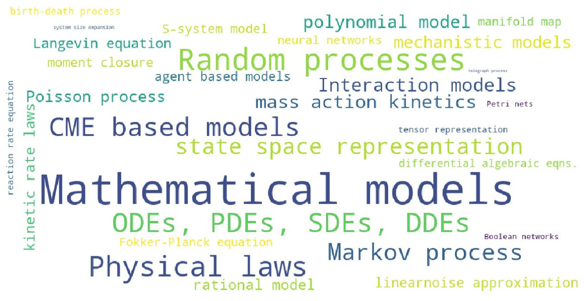 Figure 1
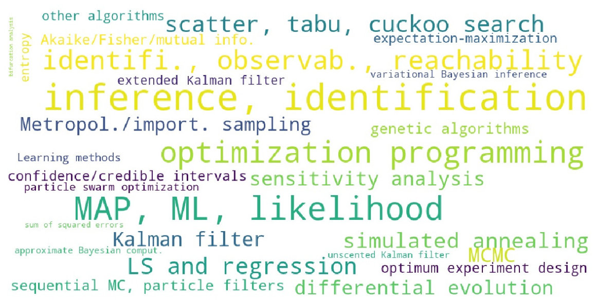 Figure 2
 Figure 3
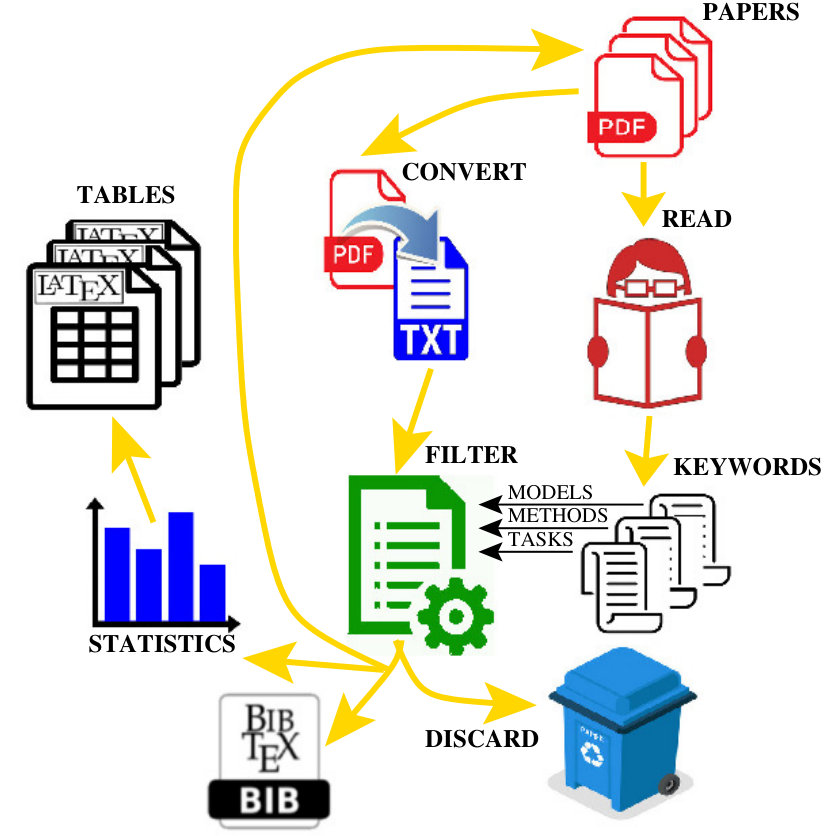 Figure 4
| Strategy | Assumptions | Objective | Estimator | Notes | |||||||||
| MMSE | , |
|
|||||||||||
| MAP | , | solve | |||||||||||
| MVUB |
|
|
|
||||||||||
| ML |
|
|
|
||||||||||
| LS |
|
|
|||||||||||
| MM |
|
asymptotically unbiased | |||||||||||
|
|||||||||||||
| Strategy | Motivation and key papers | |||
|---|---|---|---|---|
| Physical laws |
|
|||
| • kinetic rate laws |
|
|||
| • mass action kinetics |
|
|||
| • mechanistic models |
|
|||
| Random processes |
|
|||
| • Markov process |
|
|||
| • Poisson process |
|
|||
| • birth-death process |
|
|||
| • telegraph process | Veerman et al. (2018); Weber and Frey (2017) | |||
| Mathematical models | adopted models for dynamic systems | |||
| • quasi-state models |
|
|||
| • state space representation |
|
|||
| • ODEs, PDEs, SDEs, DDEs |
|
|||
| • path integral form of ODEs | Weber and Frey (2017) | |||
| • rational model |
|
|||
| • differential algebraic eqns. |
|
|||
| • tensor representation | Liao et al. (2015a); Wong et al. (2015); Smith and Grima (2018) | |||
| • S-system model |
|
|||
| • polynomial model |
|
|||
| • manifold map |
|
| Strategy | Motivation and key papers | |||
|---|---|---|---|---|
| Interaction models | qualitative modeling of chemical interactions | |||
| • Petri nets | Voit (2013); Chou and Voit (2009); Liu et al. (2012) | |||
| • Boolean networks | Emmert-Streib et al. (2012); Chou and Voit (2009) | |||
| • neural networks |
|
|||
| • agent based models |
|
|||
| CME based models | stochastic and deterministic approximations of CME | |||
| • Langevin equation |
|
|||
| • Fokker-Planck equation | Weber and Frey (2017); Schnoerr et al. (2017); Liao et al. (2015a) | |||
| • reaction rate equation |
|
|||
| • moment closure |
|
|||
| • linear noise approximation |
|
|||
| • system size expansion | Schnoerr et al. (2017); Fröhlich et al. (2016) |
|
|
|
|
|
|||||||||||||||||||||||||||||||
|
kinetic rate laws |
mass action kinetics |
mechanistic models |
Markov process |
Poisson process |
birth-death process |
telegraph process |
state space representation |
ODEs, PDEs, SDEs, DDEs |
rational model |
differential algebraic eqns. |
tensor representation |
S-system model |
polynomial model |
manifold map |
Petri nets |
Boolean networks |
neural networks |
agent based models |
Langevin equation |
Fokker-Planck equation |
reaction rate equation |
moment closure |
linear noise approximation |
system size expansion |
|||||||||||
| # papers | 59 | 104 | 82 | 166 | 72 | 22 | 2 | 150 | 216 | 58 | 27 | 19 | 39 | 89 | 35 | 13 | 13 | 36 | 43 | 55 | 35 | 19 | 45 | 50 | 4 | ||||||||||
|
|
|
|
|
|||||||||||||||||||||||||||||||
| Year |
kinetic rate laws |
mass action kinetics |
mechanistic models |
Markov process |
Poisson process |
birth-death process |
telegraph process |
state space representation |
ODEs, PDEs, SDEs, DDEs |
rational model |
differential algebraic eqns. |
tensor representation |
S-system model |
polynomial model |
manifold map |
Petri nets |
Boolean networks |
neural networks |
agent based models |
Langevin equation |
Fokker-Planck equation |
reaction rate equation |
moment closure |
linear noise approximation |
system size expansion |
||||||||||
| 2005 | 3 | 3 | 1 | 2 | 2 | . | . | 4 | 5 | . | 2 | . | . | . | . | . | . | . | . | 1 | 2 | . | . | . | . | ||||||||||
| 2006 | 2 | 4 | 2 | 2 | . | . | . | 2 | 3 | 4 | 1 | . | 1 | 3 | . | . | . | 2 | . | . | . | . | . | . | . | ||||||||||
| 2007 | . | 4 | 1 | 3 | 2 | . | . | 2 | 6 | 1 | 1 | . | 2 | 4 | 2 | . | . | 1 | 1 | 1 | . | . | . | . | . | ||||||||||
| 2008 | 1 | 4 | 2 | 2 | 1 | . | . | 6 | 6 | 1 | 1 | . | 2 | 2 | 1 | . | . | 2 | . | . | . | 1 | . | . | . | ||||||||||
| 2009 | 4 | 7 | 2 | 5 | 1 | . | . | 6 | 11 | 1 | 2 | 1 | 4 | 2 | 2 | 2 | 2 | 2 | 3 | 1 | 1 | . | . | 1 | . | ||||||||||
| 2010 | 7 | 11 | 5 | 12 | 3 | 1 | . | 8 | 13 | 6 | 2 | . | 4 | 5 | 5 | 1 | 1 | 2 | 5 | 7 | 2 | 1 | . | 2 | . | ||||||||||
| 2011 | 5 | 4 | 5 | 11 | 4 | . | . | 10 | 13 | 2 | . | . | 3 | 4 | 1 | . | . | 2 | 2 | 4 | 2 | 2 | 2 | 2 | . | ||||||||||
| 2012 | 6 | 11 | 6 | 21 | 11 | 3 | . | 14 | 19 | 5 | 4 | 1 | 5 | 6 | 3 | 2 | 3 | 6 | 6 | 9 | 6 | 1 | 4 | 9 | . | ||||||||||
| 2013 | 7 | 9 | 12 | 16 | 8 | 3 | . | 17 | 26 | 9 | 3 | 1 | 7 | 12 | 4 | 2 | . | 3 | 7 | 6 | 2 | 2 | 4 | 4 | . | ||||||||||
| 2014 | 8 | 13 | 14 | 33 | 11 | 4 | . | 26 | 33 | 7 | 4 | 2 | 5 | 14 | 2 | 1 | 3 | 7 | 6 | 7 | 5 | 5 | 10 | 9 | . | ||||||||||
| 2015 | 6 | 10 | 8 | 15 | 5 | 2 | . | 20 | 24 | 5 | 1 | 2 | 3 | 10 | 4 | 2 | 1 | 1 | 2 | 4 | 4 | . | 6 | 5 | . | ||||||||||
| 2016 | 4 | 8 | 13 | 19 | 5 | 2 | . | 14 | 23 | 4 | 1 | 2 | 3 | 10 | 5 | 1 | 2 | 4 | 7 | 6 | 3 | 3 | 7 | 8 | 2 | ||||||||||
| 2017 | 4 | 8 | 8 | 13 | 10 | 6 | 1 | 12 | 18 | 7 | 4 | 7 | . | 10 | 6 | 1 | 1 | 3 | 3 | 5 | 5 | 2 | 8 | 5 | 2 | ||||||||||
| 2018 | 2 | 8 | 3 | 11 | 8 | 1 | 1 | 7 | 13 | 5 | . | 3 | . | 5 | . | 1 | . | 1 | 1 | 4 | 3 | 2 | 4 | 5 | . | ||||||||||
| Reference | Focus | ||||
|---|---|---|---|---|---|
| (Banga and Canto, 2008) |
|
||||
| (Chou and Voit, 2009) |
|
||||
| (Ashyraliyev et al., 2009) |
|
||||
| (Smet and Marchal, 2010) |
|
||||
| (Tenazinha and Vinga, 2011) |
|
||||
| (Goutsias and Jenkinson, 2012) |
|
||||
| (Emmert-Streib et al., 2012) |
|
||||
| (Sun et al., 2012) |
|
||||
| (Kuwahara et al., 2013) |
|
||||
| (Voit, 2013) |
|
||||
| (Baker et al., 2015) |
|
||||
| (McGoff et al., 2015) |
|
||||
| (Weiss et al., 2016) | survey of transfer learning methods | ||||
| (Schnoerr et al., 2017) |
|
||||
| (Camacho et al., 2018) |
|
||||
| (Smith and Grima, 2018) |
|
| Thesis | Main research problems considered | ||
|---|---|---|---|
| (Dargatz, 2010) | Bayesian inference for biochemical models involving diffusion | ||
| (Mu, 2010) | rate and state estimation in S-system and linear fractional model (LFM) | ||
| (Palmisano, 2010) | software tools for modeling and parameter estimation in BRNs | ||
| (Mazur, 2012) | inference via stochastic sampling and Bayesian learning framework | ||
| (Srivastava, 2012) |
|
||
| (Gupta, 2013) |
|
||
| (Hasenauer, 2013) |
|
||
| (Linder, 2013) |
|
||
| (Flassig, 2014) | model identification for large scale gene regulatory networks | ||
| (Liu, 2014) | approximate Bayesian inference methods and sensitivity analysis | ||
| (Moritz, 2014) |
|
||
| (Paul, 2014) | analysis of MCMC based methods | ||
| (Ruess, 2014) |
|
||
| (Schenkendorf, 2014) |
|
||
| (Smadbeck, 2014) |
|
||
| (Schnoerr, 2016) |
|
||
| (Zechner, 2014) | inference from heterogeneous snapshot and time-lapse data | ||
| (Galagali, 2016) |
|
||
| (Hussain, 2016) |
|
||
| (Lakatos, 2017) | multivariate moment closure and reachability analysis | ||
| (Liao, 2017) | tensor representation and analysis of BRNs |
| Algorithm | Motivation and selected papers | ||
|---|---|---|---|
| Genetic algorithms (GAs) |
|
||
|
|||
| Genetic programming (GP) |
|
||
| Nobile et al. (2013); Chou and Voit (2009); Sun et al. (2012) | |||
| Evolutionary programming (EP) |
|
||
| Baker et al. (133, 2010); Sun et al. (2012); Revell and Zuliani (2018) | |||
| Simulated annealing (SA) |
|
||
|
|||
| Differential evolution (DE) |
|
||
|
|||
| Scatter search (SS) |
|
||
|
|||
| Particle swarm optimiz. (PSO) |
|
||
|
| Tasks | Measures |
|
|
|
Model fitting | XLR | ||||||||||||||||||||||||||||
|
identifi., observab., reachability |
optimum experiment design |
bifurcation analysis |
inference, identification |
sensitivity analysis |
confidence/credible intervals |
Akaike/Fisher/mutual info. |
entropy |
sum of squared errors |
MAP, ML, likelihood |
approximate Bayesian comput. |
expectation-maximization |
variational Bayesian inference |
MCMC |
Metropol./import. sampling |
sequential MC, particle filters |
Kalman filter |
extended Kalman filter |
unscented Kalman filter |
LS and regression |
genetic algorithms |
optimization programming |
simulated annealing |
differential evolution |
scatter, tabu, cuckoo search |
particle swarm optimization |
other algorithms |
mach./deep/transf. learning |
|||||||
| # papers | 149 | 61 | 9 | 288 | 81 | 63 | 68 | 50 | 21 | 233 | 30 | 57 | 33 | 82 | 78 | 77 | 87 | 53 | 30 | 110 | 77 | 191 | 97 | 83 | 113 | 40 | 56 | 45 | ||||||
| Tasks | Measures |
|
|
|
Model fitting | XLR | ||||||||||||||||||||||||||||
| Year |
identifi., observab., reachability |
optimum experiment design |
bifurcation analysis |
inference, identification |
sensitivity analysis |
confidence/credible intervals |
Akaike/Fisher/mutual info. |
entropy |
sum of squared errors |
MAP, ML, likelihood |
approximate Bayesian comput. |
expectation-maximization |
variational Bayesian inference |
MCMC |
Metropol./import. sampling |
sequential MC, particle filters |
Kalman filter |
extended Kalman filter |
unscented Kalman filter |
LS and regression |
genetic algorithms |
optimization programming |
simulated annealing |
differential evolution |
scatter, tabu, cuckoo search |
particle swarm optimization |
other algorithms |
mach./deep/transf. learning |
||||||
| 2005 | 3 | 2 | . | 7 | 1 | 1 | 1 | . | . | 3 | . | . | . | 2 | 2 | 1 | 2 | . | . | 1 | 1 | 3 | 1 | 1 | . | . | . | . | ||||||
| 2006 | 6 | 1 | . | 10 | 1 | 4 | 2 | . | 2 | 7 | . | 1 | 1 | . | . | . | . | . | . | 4 | 3 | 4 | 4 | 6 | 1 | . | 2 | 1 | ||||||
| 2007 | 2 | 2 | 1 | 8 | 1 | 2 | 1 | . | 2 | 5 | . | . | . | 1 | 1 | 2 | 2 | 1 | 1 | 4 | 4 | 5 | 4 | 3 | 1 | 1 | 2 | 2 | ||||||
| 2008 | 3 | 3 | . | 9 | 1 | 1 | 1 | . | 1 | 6 | . | 2 | . | 1 | 1 | 1 | 2 | 1 | 1 | 5 | 3 | 7 | 3 | 5 | 4 | . | 2 | 1 | ||||||
| 2009 | 8 | 4 | 1 | 13 | 4 | 4 | 4 | 2 | 1 | 11 | 1 | . | 2 | 3 | 3 | 2 | 4 | 1 | 2 | 7 | 8 | 9 | 7 | 7 | 6 | 3 | 4 | 1 | ||||||
| 2010 | 13 | 5 | . | 22 | 8 | 4 | 8 | 3 | 2 | 18 | 3 | 4 | 2 | 5 | 8 | 6 | 5 | 3 | 1 | 7 | 7 | 16 | 10 | 8 | 6 | 2 | 3 | 3 | ||||||
| 2011 | 9 | 5 | . | 18 | 6 | 3 | 2 | 1 | . | 15 | 1 | 4 | 2 | 6 | 7 | 4 | 4 | 4 | 2 | 4 | 4 | 11 | 6 | 4 | 6 | 2 | 2 | . | ||||||
| 2012 | 14 | 7 | 3 | 25 | 10 | 5 | 10 | 6 | . | 21 | 2 | 9 | 3 | 8 | 12 | 9 | 5 | 2 | 2 | 11 | 8 | 17 | 10 | 10 | 12 | 4 | 7 | 4 | ||||||
| 2013 | 19 | 6 | 2 | 30 | 11 | 6 | 11 | 8 | 3 | 28 | 3 | 4 | 4 | 12 | 6 | 10 | 14 | 11 | 2 | 14 | 12 | 21 | 9 | 7 | 15 | 10 | 7 | 8 | ||||||
| 2014 | 27 | 12 | 1 | 45 | 13 | 17 | 12 | 10 | 4 | 40 | 6 | 14 | 10 | 20 | 14 | 19 | 19 | 12 | 8 | 21 | 11 | 27 | 15 | 9 | 18 | 5 | 10 | 8 | ||||||
| 2015 | 16 | 3 | . | 27 | 8 | 4 | 3 | 4 | 1 | 22 | 5 | 8 | 1 | 9 | 7 | 10 | 13 | 8 | 7 | 11 | 4 | 19 | 7 | 4 | 8 | 3 | 4 | 3 | ||||||
| 2016 | 12 | 2 | 1 | 27 | 9 | 5 | 5 | 4 | 3 | 23 | 3 | 4 | 1 | 7 | 6 | 4 | 8 | 4 | 1 | 10 | 6 | 17 | 9 | 8 | 13 | 6 | 6 | 7 | ||||||
| 2017 | 10 | 7 | . | 23 | 7 | 6 | 4 | 5 | 2 | 15 | 3 | 3 | 5 | 4 | 5 | 3 | 4 | 2 | 1 | 6 | 3 | 19 | 7 | 8 | 15 | 4 | 5 | 2 | ||||||
| 2018 | 7 | 2 | . | 19 | 1 | 1 | 4 | 7 | . | 16 | 3 | 3 | 1 | 4 | 5 | 6 | 3 | 2 | 2 | 4 | 2 | 12 | 4 | 2 | 7 | . | 2 | 4 | ||||||
| Tasks | Measures |
|
|
|
Model fitting | XLR | |||||||||||||||||||||||||||||
|
identifi., observab., reachability |
optimum experiment design |
bifurcation analysis |
inference, identification |
sensitivity analysis |
confidence/credible intervals |
Akaike/Fisher/mutual info. |
entropy |
sum of squared errors |
MAP, ML, likelihood |
approximate Bayesian comput. |
expectation-maximization |
variational Bayesian inference |
MCMC |
Metropol./import. sampling |
sequential MC, particle filters |
Kalman filter |
extended Kalman filter |
unscented Kalman filter |
LS and regression |
genetic algorithms |
optimization programming |
simulated annealing |
differential evolution |
scatter, tabu, cuckoo search |
particle swarm optimization |
other algorithms |
mach./deep/transf. learning |
||||||||
| Physical laws | kinetic rate laws | 3 | 2 | . | 10 | 3 | 1 | . | 2 | . | 6 | 1 | . | 1 | 1 | . | 2 | 2 | 2 | 2 | 3 | 2 | 4 | 1 | 3 | 3 | 1 | 2 | . | ||||||
| mass action kinetics | 7 | 2 | . | 19 | 2 | 1 | . | 2 | 1 | 11 | . | 3 | 2 | 4 | 1 | . | . | . | . | 4 | 2 | 4 | 2 | 3 | 2 | 1 | 2 | . | |||||||
| mechanistic models | 5 | . | . | 15 | 2 | 5 | 1 | 1 | 1 | 12 | 3 | 3 | . | 3 | 1 | 3 | 1 | 1 | . | 2 | 1 | 4 | 2 | 2 | 2 | 2 | 2 | 1 | |||||||
| Random processes | Markov process | 22 | 3 | 1 | 99 | 10 | 11 | 8 | 9 | 1 | 85 | 15 | 7 | 7 | 49 | 30 | 27 | 11 | 4 | 3 | 16 | 3 | 12 | 5 | 3 | 7 | . | 3 | 4 | ||||||
| Poisson process | 6 | 2 | 1 | 22 | 4 | 2 | 3 | 6 | 1 | 17 | 2 | 3 | 4 | 12 | 9 | 4 | 2 | . | . | 4 | 2 | 4 | . | 1 | 3 | . | 1 | . | |||||||
| birth-death process | 3 | 1 | . | 9 | 1 | 1 | . | 1 | . | 8 | . | 1 | 2 | 3 | 2 | 1 | . | . | . | . | . | . | . | . | 1 | . | . | . | |||||||
| telegraph process | . | . | . | 2 | . | . | . | . | . | 1 | . | . | 1 | . | . | . | . | . | . | . | . | . | . | . | 1 | . | . | . | |||||||
| Mathematical models | state space representation | 16 | 5 | 1 | 53 | 7 | 4 | 5 | 6 | 1 | 45 | 5 | 5 | 3 | 15 | 13 | 14 | 15 | 7 | 7 | 7 | 2 | 8 | 3 | 1 | 5 | . | 2 | 2 | ||||||
| ODEs, PDEs, SDEs, DDEs | 43 | 8 | 1 | 132 | 16 | 15 | 12 | 8 | 3 | 90 | 8 | 14 | 6 | 32 | 16 | 20 | 19 | 12 | 9 | 19 | 8 | 25 | 11 | 15 | 14 | 9 | 7 | 3 | |||||||
| rational model | 4 | . | . | 6 | 2 | 2 | 1 | . | . | 5 | 2 | 1 | . | 2 | 2 | 4 | 1 | 1 | 1 | 2 | 1 | 3 | 3 | 1 | 1 | . | 1 | 2 | |||||||
| differential algebraic equations | 4 | 1 | . | 6 | 1 | 1 | . | . | . | 4 | 1 | . | . | . | 1 | . | 1 | . | . | 3 | 3 | 3 | 2 | 2 | . | 1 | . | . | |||||||
| tensor representation | 3 | 2 | . | 4 | 2 | 1 | 1 | 1 | . | 3 | . | . | . | . | . | . | 1 | 1 | 1 | 1 | . | . | 1 | . | . | . | 1 | . | |||||||
| S-system model | 4 | 2 | 1 | 25 | 3 | 2 | 1 | 2 | . | 9 | . | 2 | 2 | 2 | 1 | . | 3 | 3 | 2 | 11 | 5 | 6 | 3 | 7 | . | 2 | 2 | . | |||||||
| polynomial model | 10 | 3 | 1 | 25 | 5 | 4 | 2 | 3 | 1 | 12 | 1 | 2 | 2 | 5 | 4 | 1 | 2 | 1 | 2 | 8 | 2 | 11 | . | 2 | 1 | . | 2 | . | |||||||
| manifold map | 3 | . | . | 7 | 2 | 1 | . | 1 | . | 6 | 3 | 2 | . | 3 | 2 | 4 | 3 | 2 | 2 | 4 | . | . | 1 | . | 1 | . | 2 | 2 | |||||||
| Interaction models | Petri nets | 1 | . | 1 | 3 | 2 | . | 1 | 2 | . | 2 | . | 1 | . | 1 | 1 | . | . | . | . | 1 | 1 | 1 | . | . | . | . | 1 | . | ||||||
| Boolean networks | 2 | . | 1 | 2 | 1 | 1 | 2 | 1 | . | 2 | . | 1 | . | 1 | 1 | 1 | . | . | . | 2 | 1 | 2 | . | 1 | . | . | . | 1 | |||||||
| neural networks | 3 | . | . | 9 | 3 | 1 | 1 | 2 | . | 5 | 1 | 1 | . | 1 | 1 | 1 | 3 | 3 | 3 | 5 | 2 | 2 | 2 | 1 | 1 | 1 | 9 | 3 | |||||||
| agent based models | 2 | . | 1 | 9 | 2 | 1 | 1 | 2 | . | 7 | 1 | 2 | . | 3 | 3 | 5 | 2 | . | . | 1 | 2 | 3 | 2 | . | 2 | . | 1 | . | |||||||
| CME based models | Langevin equation | 4 | 1 | . | 17 | 4 | 2 | 2 | 3 | 1 | 15 | . | . | 3 | 9 | 8 | 4 | 3 | 1 | . | . | . | 2 | 1 | . | 3 | . | 1 | . | ||||||
| Fokker-Planck equation | 5 | 2 | . | 11 | 1 | 2 | 2 | 2 | 1 | 9 | . | . | 4 | 4 | 2 | 1 | 1 | . | . | . | . | 1 | . | . | 3 | . | . | . | |||||||
| reaction rate equation | 3 | 1 | . | 3 | 1 | 1 | 1 | . | . | 3 | . | . | . | 2 | 1 | . | 1 | . | . | . | . | 1 | . | . | 2 | . | . | . | |||||||
| moment closure | 8 | . | . | 24 | 4 | 1 | 3 | 5 | 2 | 17 | 1 | 1 | 4 | 5 | 2 | 3 | 2 | 1 | . | 1 | . | 2 | . | . | 5 | . | 1 | 1 | |||||||
| linear noise approximation | 10 | 1 | . | 29 | 6 | 3 | 4 | 4 | 2 | 25 | 2 | 2 | 1 | 12 | 5 | 6 | 2 | . | . | 1 | . | . | . | 1 | 5 | . | 1 | . | |||||||
| system size expansion | 2 | 1 | . | 4 | 1 | 1 | . | 1 | 2 | 4 | . | 1 | 1 | 2 | . | . | . | . | . | . | . | . | . | . | 1 | . | . | . | |||||||
| Measures |
|
|
|
Model fitting | XLR | |||||||||||||||||||||||||
|
confidence/credible intervals |
Akaike/Fisher/mutual info. |
entropy |
sum of squared errors |
MAP, ML, likelihood |
approximate Bayesian comput. |
expectation-maximization |
variational Bayesian inference |
MCMC |
Metropol./import. sampling |
sequential MC, particle filters |
Kalman filter |
extended Kalman filter |
unscented Kalman filter |
LS and regression |
genetic algorithms |
optimization programming |
simulated annealing |
differential evolution |
searches |
particle swarm optimiz. |
other algorithms |
mach./deep/transf. learning |
||||||||
| Tasks | identifi., observab., reachability | 44 | 54 | 28 | 10 | 131 | 20 | 25 | 21 | 45 | 37 | 43 | 49 | 27 | 15 | 71 | 42 | 96 | 56 | 45 | 60 | 19 | 23 | 26 | ||||||
| bifurcation analysis | 16 | 15 | 15 | 9 | 55 | 10 | 17 | 11 | 25 | 24 | 23 | 16 | 8 | 4 | 27 | 21 | 48 | 30 | 16 | 25 | 10 | 11 | 9 | |||||||
| optimum experiment | 4 | 7 | 3 | 2 | 9 | . | 4 | 2 | 2 | 3 | 2 | 3 | 1 | 1 | 5 | 4 | 7 | 4 | 5 | 4 | 2 | 5 | 3 | |||||||
| inference, identification | 63 | 68 | 50 | 21 | 233 | 30 | 57 | 33 | 82 | 78 | 77 | 87 | 53 | 30 | 110 | 77 | 191 | 97 | 83 | 113 | 40 | 56 | 45 | |||||||
| sensitivity analysis | 25 | 36 | 19 | 6 | 71 | 13 | 24 | 15 | 22 | 21 | 27 | 28 | 17 | 12 | 44 | 28 | 63 | 37 | 29 | 35 | 13 | 14 | 16 | |||||||
|
|
|
|
|
|||||||||||||||||||||||||||||||
| Reference |
kinetic rate laws |
mass action kinetics |
mechanistic models |
Markov process |
Poisson process |
birth-death process |
telegraph process |
state space representation |
ODEs, PDEs, SDEs, DDEs |
rational model |
differential algebraic eqns. |
tensor representation |
S-system model |
polynomial model |
manifold map |
Petri nets |
Boolean networks |
neural networks |
agent based models |
Langevin equation |
Fokker-Planck equation |
reaction rate equation |
moment closure |
linear noise approximation |
system size expansion |
||||||||||
| Abdullah et al. (2013c) | . | . | . | . | . | . | . | 1 | 1 | 1 | 1 | . | . | . | . | . | . | . | . | . | . | . | . | . | . | ||||||||||
| Abdullah et al. (2013b) | . | . | . | . | . | . | . | 2 | 4 | 4 | . | . | . | 1 | . | . | . | . | 1 | . | . | . | . | . | . | ||||||||||
| Abdullah et al. (2013a) | . | . | . | . | . | . | . | . | 7 | 1 | . | . | . | . | . | . | . | . | 3 | . | . | . | . | . | . | ||||||||||
| Alberton et al. (2013) | . | . | 1 | . | . | . | . | . | . | . | . | . | . | . | . | . | . | 1 | . | . | . | . | . | . | . | ||||||||||
| Ale et al. (2013) | 1 | . | . | . | . | . | . | . | 10 | . | . | . | . | 3 | . | . | . | . | . | . | . | . | 7 | 15 | . | ||||||||||
| Ali et al. (2015) | . | . | 2 | . | . | . | . | 4 | 1 | . | . | . | . | 3 | . | . | . | 21 | . | . | . | . | . | . | . | ||||||||||
| Amrein and Künsch (2012) | . | 2 | . | 33 | 3 | . | . | 9 | 1 | . | . | . | . | . | . | . | . | . | . | . | . | . | . | . | . | ||||||||||
| Anai et al. (2006) | . | . | . | . | . | . | . | . | 1 | . | . | . | . | 2 | . | . | . | . | . | . | . | . | . | . | . | ||||||||||
| Andreychenko et al. (2011) | . | . | . | 15 | . | . | . | 24 | 7 | . | . | . | . | . | . | . | . | . | . | . | . | . | . | . | . | ||||||||||
| Andreychenko et al. (2012) | . | . | . | 10 | . | . | . | 13 | 6 | . | . | . | . | . | . | . | . | . | . | . | . | . | . | 2 | . | ||||||||||
| Andreychenko (2014) | . | . | . | 12 | . | . | . | 12 | 4 | . | . | . | . | 3 | . | . | . | . | . | . | . | . | 33 | . | . | ||||||||||
| Andrieu et al. (2010) | . | . | 2 | 99 | 3 | . | . | 49 | . | . | . | . | . | . | 1 | . | . | . | . | 2 | . | . | . | . | . | ||||||||||
| Angius and Horváth (2011) | . | 9 | . | 4 | . | . | . | 5 | 9 | . | . | . | . | . | . | . | . | . | 9 | . | . | . | . | . | . | ||||||||||
| Arnold et al. (2014) | . | . | 1 | 3 | . | . | . | . | 5 | . | . | . | . | . | . | . | . | . | . | . | . | . | . | . | . | ||||||||||
| Ashyraliyev et al. (2009) | . | . | . | 5 | . | . | . | 1 | 1 | . | 10 | . | . | . | . | . | . | . | . | . | . | . | . | . | . | ||||||||||
| Atitey et al. (2018b) | . | . | . | 3 | . | . | . | . | . | . | . | 1 | . | . | . | . | . | . | . | . | . | . | . | . | . | ||||||||||
| Atitey et al. (2018a) | . | . | . | . | . | . | . | . | . | 1 | . | . | . | . | . | . | . | . | . | . | . | . | . | . | . | ||||||||||
| Atitey et al. (2019) | . | . | . | . | 2 | . | . | . | 1 | 1 | . | . | . | . | . | . | . | . | . | . | . | . | . | . | . | ||||||||||
| Azab et al. (2018) | . | 1 | . | . | . | . | . | . | . | . | . | . | . | . | . | . | . | . | . | . | . | . | . | . | . | ||||||||||
| Babtie and Stumpf (2017) | . | . | 7 | 1 | . | . | . | . | 4 | 1 | . | . | . | . | 1 | . | . | . | . | . | . | . | . | . | . | ||||||||||
| Backenköhler et al. (2016) | . | 6 | . | 3 | . | . | . | 4 | 1 | . | . | . | . | 2 | . | . | . | . | . | . | . | . | 7 | . | . | ||||||||||
| Backenköhler et al. (2018) | . | 7 | . | 3 | 1 | 1 | . | 4 | 1 | 1 | . | . | . | 2 | . | . | . | . | . | . | . | . | 8 | . | . | ||||||||||
| Baker et al. (133, 2010) | 2 | . | . | . | . | . | . | . | 2 | 1 | 1 | . | . | . | . | . | . | . | . | . | . | . | . | . | . | ||||||||||
| Baker et al. (2011) | 8 | . | 1 | . | . | . | . | 6 | 4 | . | . | . | . | . | . | . | . | . | . | . | . | . | . | . | . | ||||||||||
| Baker et al. (2013) | 5 | . | 2 | 4 | . | . | . | 14 | 10 | . | . | . | . | . | . | . | . | . | . | . | . | . | . | . | . | ||||||||||
| Baker et al. (2015) | 4 | . | 2 | . | . | . | . | 10 | 8 | 1 | . | . | . | . | . | . | . | . | . | . | . | . | . | . | . | ||||||||||
| Banga and Canto (2008) | . | . | 2 | . | . | . | . | 1 | 3 | . | 1 | . | . | . | . | . | . | . | . | . | . | . | . | . | . | ||||||||||
| Barnes et al. (2011) | . | . | 2 | 2 | . | . | . | 1 | 1 | . | . | . | . | . | . | . | . | . | . | . | . | . | . | . | . | ||||||||||
| Bayer et al. (2015) | . | 2 | . | 19 | . | 3 | . | 6 | 20 | . | . | . | . | 2 | 3 | . | . | . | . | 1 | 2 | . | 1 | . | . | ||||||||||
| Berrones et al. (2016) | . | . | . | 2 | . | . | . | . | . | . | . | . | 3 | . | . | . | . | 2 | . | . | . | . | . | . | . | ||||||||||
| Besozzi et al. (2009) | . | . | . | . | . | . | . | . | 3 | . | . | . | . | . | . | . | . | . | 4 | . | . | . | . | . | . | ||||||||||
| Bhaskar et al. (2010) | . | . | . | 3 | . | . | . | . | 2 | . | . | . | . | . | . | . | . | . | . | . | . | . | . | . | . | ||||||||||
| Bogomolov et al. (2015) | 1 | 1 | . | 6 | . | . | . | 2 | 10 | . | . | . | . | 1 | . | . | . | . | . | . | . | . | 27 | 1 | . | ||||||||||
| Bouraoui et al. (2015) | . | . | . | . | . | . | . | 1 | . | . | . | . | . | . | . | . | . | . | . | . | . | . | . | . | . | ||||||||||
| Farza et al. (2016) | . | . | . | . | . | . | . | 1 | 4 | . | . | . | . | . | . | . | . | . | . | . | . | . | . | . | . | ||||||||||
| Boys et al. (2008) | 3 | 1 | . | 7 | 6 | . | . | 2 | . | . | . | . | . | . | . | . | . | . | . | . | . | . | . | . | . | ||||||||||
| Brim et al. (2013) | . | 7 | . | 13 | 9 | 2 | . | 25 | 12 | . | . | . | . | 4 | . | . | . | . | . | . | . | . | 2 | . | . | ||||||||||
| Bronstein et al. (2015) | . | 1 | . | 11 | 2 | . | . | 2 | 13 | . | . | . | . | . | 1 | . | . | . | . | 2 | 4 | . | 2 | 18 | . | ||||||||||
| Bronstein and Koeppl (2017) | . | 1 | . | 9 | 50 | . | . | 3 | 1 | . | . | . | . | 4 | 2 | . | . | . | . | 1 | 5 | 1 | 70 | 2 | . | ||||||||||
| Busetto and Buhmann (2009) | 1 | 2 | . | 8 | . | . | . | 4 | 2 | . | . | 2 | . | . | . | . | . | . | . | 2 | 2 | . | . | . | . | ||||||||||
| Camacho et al. (2018) | . | . | 1 | . | . | . | . | . | 1 | 2 | . | . | . | . | . | . | . | 23 | . | . | . | . | . | . | . | ||||||||||
| Balsa-Canto et al. (2008) | . | . | . | . | . | . | . | . | 1 | . | . | . | . | . | . | . | . | . | . | . | . | . | . | . | . | ||||||||||
| Carmi et al. (2013) | . | . | . | 21 | 4 | . | . | 2 | 3 | . | . | . | . | . | . | . | . | . | 63 | . | . | . | . | . | . | ||||||||||
| Cazzaniga et al. (2015) | . | . | 1 | . | . | . | . | . | 1 | . | . | . | . | . | . | . | . | . | . | . | . | . | . | . | . | ||||||||||
| Cedersund et al. (2016) | . | . | 1 | . | . | . | . | 1 | 8 | 1 | . | . | . | . | . | . | . | 3 | 1 | . | . | . | . | . | . | ||||||||||
| Česka et al. (2014) | . | 6 | . | 10 | . | 2 | . | 19 | 13 | . | . | . | . | 2 | . | . | . | . | . | . | . | . | 1 | . | . | ||||||||||
| Češka et al. (2017) | . | 2 | . | 13 | 5 | 2 | . | 3 | 8 | . | . | . | . | 28 | . | . | 1 | . | . | . | . | . | . | . | . | ||||||||||
| Chen et al. (2017) | . | . | . | . | . | . | . | . | 1 | . | . | . | . | . | . | . | . | . | . | . | . | . | 2 | . | . | ||||||||||
| Chevaliera and Samadb (2011) | . | . | . | 3 | . | . | . | . | 1 | 3 | . | . | . | 4 | . | . | . | . | . | . | . | 1 | 25 | . | . | ||||||||||
|
|
|
|
|
|||||||||||||||||||||||||||||||
| Reference |
kinetic rate laws |
mass action kinetics |
mechanistic models |
Markov process |
Poisson process |
birth-death process |
telegraph process |
state space representation |
ODEs, PDEs, SDEs, DDEs |
rational model |
differential algebraic eqns. |
tensor representation |
S-system model |
polynomial model |
manifold map |
Petri nets |
Boolean networks |
neural networks |
agent based models |
Langevin equation |
Fokker-Planck equation |
reaction rate equation |
moment closure |
linear noise approximation |
system size expansion |
||||||||||
| Chong et al. (2012) | . | . | . | . | . | . | . | . | 4 | . | . | . | 1 | . | . | . | . | 1 | . | . | . | . | . | . | . | ||||||||||
| Chong et al. (2014) | . | . | . | . | . | . | . | . | 7 | . | . | . | . | . | . | . | . | . | . | . | . | . | . | . | . | ||||||||||
| Chou et al. (2006) | 1 | . | . | . | . | . | . | . | . | . | . | . | 23 | . | . | . | . | 1 | . | . | . | . | . | . | . | ||||||||||
| Chou and Voit (2009) | 9 | 6 | 10 | . | . | . | . | . | 5 | . | . | . | 82 | . | 2 | 1 | 2 | 6 | 1 | . | . | . | . | . | . | ||||||||||
| Cseke et al. (2016) | . | . | . | 22 | . | . | . | 4 | 14 | . | . | . | . | 2 | . | . | . | . | . | 6 | 5 | . | 14 | . | . | ||||||||||
| Dai and Lai (2010) | . | . | . | . | . | . | . | . | 7 | 1 | . | . | . | . | 1 | . | . | . | . | . | . | . | . | . | . | ||||||||||
| Daigle et al. (2012) | . | 2 | 5 | 2 | 47 | 17 | . | . | . | . | . | . | . | . | . | . | . | . | . | . | . | . | . | . | . | ||||||||||
| Dargatz (2010) | . | 1 | . | 195 | 25 | . | . | 83 | 144 | . | . | . | . | 9 | 1 | . | . | . | 1 | 33 | 13 | . | . | 2 | . | ||||||||||
| Dattner (2015) | . | . | . | . | . | . | . | 1 | 28 | . | . | . | . | 15 | . | . | . | . | 1 | . | . | . | . | . | . | ||||||||||
| Deng and Tian (2014) | . | . | 1 | 1 | . | . | . | . | 3 | . | 10 | . | 2 | 1 | . | . | . | . | . | . | . | . | . | 1 | . | ||||||||||
| Dey et al. (2018) | . | 1 | . | . | . | . | . | 1 | . | . | . | . | . | . | . | . | . | . | . | 8 | 1 | . | . | . | . | ||||||||||
| Dinh and Sidje (2017) | . | . | . | 2 | . | . | . | 9 | 18 | . | . | 1 | . | . | . | . | . | . | . | . | . | . | . | . | . | ||||||||||
| Dochain (2003) | . | . | . | . | . | . | . | 2 | . | . | . | . | . | 1 | . | . | . | . | . | . | . | . | . | . | . | ||||||||||
| Drovandi et al. (2016) | . | 1 | . | 36 | 4 | . | . | 2 | . | . | . | . | . | . | . | . | . | . | . | . | . | . | . | 1 | . | ||||||||||
| Eghtesadi and Mcauley (2014) | . | . | 3 | . | . | . | . | . | . | . | 2 | . | . | . | . | . | . | . | 1 | . | . | . | . | . | . | ||||||||||
| Eisenberg and Hayashi (2014) | . | . | . | . | . | . | . | 1 | 10 | . | . | . | . | . | . | . | . | . | . | . | . | . | . | . | . | ||||||||||
| Engl et al. (2009) | 20 | 7 | . | . | . | . | . | 1 | 44 | . | . | . | 6 | . | 3 | . | 1 | . | . | . | . | . | . | . | . | ||||||||||
| Erguler and Stumpf (2011) | . | . | 4 | . | . | . | . | . | 8 | . | . | . | . | . | . | . | . | . | . | . | . | . | . | . | . | ||||||||||
| Fages et al. (2015) | 1 | 4 | . | 1 | . | . | . | . | 91 | . | . | . | . | 8 | . | 8 | . | . | . | . | . | . | . | . | . | ||||||||||
| Famili et al. (2005) | 6 | 2 | 2 | . | . | . | . | . | . | . | . | . | . | . | . | . | . | . | . | . | . | . | . | . | . | ||||||||||
| Farina et al. (2006) | . | 9 | . | . | . | . | . | 1 | . | 1 | . | . | . | 1 | . | . | . | . | . | . | . | . | . | . | . | ||||||||||
| Fearnhead and Prangle (2012) | . | . | 1 | 39 | 1 | . | . | 3 | . | . | . | . | . | 4 | . | . | . | 4 | . | . | . | . | . | . | . | ||||||||||
| Fearnhead et al. (2014) | . | . | . | 7 | 3 | . | . | 4 | 86 | . | . | . | . | . | . | . | . | . | . | . | . | . | . | 125 | . | ||||||||||
| Rodriguez-Fernandez et al. (2006b) | . | . | . | . | . | . | . | 2 | 7 | . | 2 | . | . | . | . | . | . | . | . | . | . | . | . | . | . | ||||||||||
| Rodriguez-Fernandez et al. (2006a) | . | . | 1 | . | . | . | . | . | 3 | . | 2 | . | . | . | . | . | . | . | . | . | . | . | . | . | . | ||||||||||
| Rodriguez-Fernandez et al. (2013) | . | . | . | 1 | . | . | . | . | 2 | . | 6 | . | . | . | . | . | . | . | . | . | . | . | . | . | . | ||||||||||
| Fey et al. (2008) | . | 2 | . | . | . | . | . | 1 | 1 | . | . | . | . | . | 1 | . | . | . | . | . | . | . | . | . | . | ||||||||||
| Fey and Bullinger (2010) | . | 4 | . | . | . | . | . | . | 1 | . | . | . | . | 18 | . | . | . | . | . | . | . | . | . | . | . | ||||||||||
| Flassig (2014) | 2 | . | 5 | 5 | . | . | . | 1 | 71 | 16 | . | . | . | 4 | 1 | . | 7 | . | . | . | . | . | . | . | . | ||||||||||
| Folia and Rattray (2018) | . | . | . | 8 | . | . | . | . | 31 | . | . | . | . | . | . | . | . | . | . | . | . | . | . | 29 | . | ||||||||||
| Fröhlich et al. (2014) | . | . | . | 7 | . | . | . | . | 10 | . | . | . | . | . | . | . | . | . | . | . | . | . | . | . | . | ||||||||||
| Fröhlich et al. (2016) | . | . | 6 | 3 | . | . | . | . | 9 | . | . | 3 | . | . | 1 | . | . | . | 2 | 1 | 1 | 2 | 5 | 41 | 50 | ||||||||||
| Fröhlich et al. (2017) | 1 | 1 | 11 | 1 | . | . | . | . | 16 | 3 | 1 | 1 | . | 1 | 3 | . | . | . | . | 2 | . | . | . | . | . | ||||||||||
| Gábor and Banga (2014) | . | . | . | . | . | . | . | . | 3 | . | . | . | . | . | . | . | . | . | . | . | . | . | . | . | . | ||||||||||
| Gábor et al. (2017) | . | . | 2 | . | . | . | . | . | 3 | 1 | . | . | . | . | . | . | . | . | . | . | . | . | . | . | . | ||||||||||
| Galagali (2016) | . | 11 | 1 | 46 | 3 | . | . | 7 | 20 | . | . | . | . | . | . | . | 2 | . | . | 1 | . | . | . | 1 | . | ||||||||||
| Geffen et al. (2008) | . | 1 | . | . | . | . | . | 2 | . | . | . | . | . | . | . | . | . | . | . | . | . | . | . | . | . | ||||||||||
| Gennemark and Wedelin (2007) | . | . | . | . | . | . | . | . | 20 | . | . | . | 10 | 3 | . | . | . | . | . | . | . | . | . | . | . | ||||||||||
| Ghusinga et al. (2017) | 1 | . | . | . | 1 | . | . | 1 | . | . | . | . | . | 5 | . | . | . | 1 | . | . | . | . | 19 | . | . | ||||||||||
| Gillespie and Golightly (2012) | . | 1 | . | 5 | 1 | . | . | . | 24 | . | . | . | . | . | . | . | . | . | . | . | . | . | 1 | . | . | ||||||||||
| Golightly and Wilkinson (2006) | 1 | 2 | . | 6 | 1 | . | . | . | 3 | . | . | . | . | . | . | . | . | . | . | . | 2 | . | . | . | . | ||||||||||
| Golightly and Wilkinson (2005) | 1 | 4 | . | 12 | 2 | . | . | . | 9 | . | . | . | . | . | . | . | . | . | . | 1 | 4 | . | . | . | . | ||||||||||
| Golightly and Wilkinson (2011) | 2 | 1 | 1 | 24 | 1 | . | . | 4 | 9 | . | . | . | . | . | . | . | . | . | . | 4 | 2 | . | . | . | . | ||||||||||
| Golightly et al. (2012) | . | . | . | 23 | 2 | . | . | 2 | 15 | . | . | . | . | . | . | . | . | . | . | 8 | . | . | . | 76 | . | ||||||||||
| Golightly et al. (2015) | 1 | 1 | . | 26 | 4 | . | . | 3 | 16 | . | . | . | . | . | . | . | . | . | . | 8 | . | . | . | 109 | . | ||||||||||
| Golightly and Kypraios (2017) | . | 1 | . | 20 | 1 | . | . | 3 | . | . | . | . | . | . | . | . | . | . | . | . | . | . | . | . | . | ||||||||||
| Golightly et al. (2018) | 1 | 1 | . | 16 | 28 | . | . | 2 | 4 | . | . | . | . | . | . | . | . | . | . | 7 | . | . | . | . | . | ||||||||||
| González et al. (2013) | . | . | . | . | . | . | . | 2 | 27 | . | . | . | 5 | . | 2 | . | . | 1 | . | 1 | . | . | . | . | . | ||||||||||
| Gordon et al. (1993) | . | . | . | 1 | . | . | . | 9 | . | . | . | . | . | . | . | . | . | . | . | . | . | . | . | . | . | ||||||||||
|
|
|
|
|
|||||||||||||||||||||||||||||||
| Reference |
kinetic rate laws |
mass action kinetics |
mechanistic models |
Markov process |
Poisson process |
birth-death process |
telegraph process |
state space representation |
ODEs, PDEs, SDEs, DDEs |
rational model |
differential algebraic eqns. |
tensor representation |
S-system model |
polynomial model |
manifold map |
Petri nets |
Boolean networks |
neural networks |
agent based models |
Langevin equation |
Fokker-Planck equation |
reaction rate equation |
moment closure |
linear noise approximation |
system size expansion |
||||||||||
| Guillén-Gosálbez et al. (2013) | 3 | . | 1 | . | . | . | . | . | 1 | . | . | . | 2 | . | . | . | . | . | . | . | . | . | . | . | . | ||||||||||
| Goutsias and Jenkinson (2012) | 1 | 2 | . | 139 | 24 | . | . | 12 | 1 | . | . | . | . | 2 | . | 8 | . | 20 | 10 | 15 | 2 | . | 13 | 22 | . | ||||||||||
| Gratie et al. (2013) | . | 5 | 4 | 8 | . | . | . | 1 | 55 | 1 | . | . | . | 1 | . | 2 | . | . | 1 | . | . | . | . | . | . | ||||||||||
| Gupta (2013) | . | 2 | 1 | 72 | 6 | . | . | 17 | 48 | . | . | . | . | 1 | . | . | . | . | . | . | . | . | . | . | . | ||||||||||
| Gupta and Rawlings (2014) | . | 2 | 1 | 17 | . | . | . | 11 | 4 | 1 | . | . | . | . | . | . | . | . | . | . | . | . | . | . | . | ||||||||||
| Hagen et al. (2013) | . | 1 | 4 | . | . | . | . | . | 6 | 4 | . | . | . | . | . | . | . | . | . | . | . | . | . | 2 | . | ||||||||||
| Hasenauer et al. (2010) | . | 2 | . | . | . | . | . | . | . | 1 | . | . | . | 9 | . | . | . | . | . | . | . | . | . | . | . | ||||||||||
| Hasenauer (2013) | 3 | 3 | 12 | 43 | 1 | 4 | . | 2 | 99 | 3 | . | . | . | 6 | 2 | . | . | . | 2 | 21 | 30 | 10 | 1 | . | . | ||||||||||
| Mustafa et al. (2013) | . | . | . | 1 | . | . | . | . | . | . | . | . | . | . | . | . | . | . | . | . | . | . | . | . | . | ||||||||||
| Th and Manini (2008) | . | . | . | 2 | . | . | . | 1 | 12 | . | . | . | . | . | . | . | . | . | . | . | . | . | . | . | . | ||||||||||
| Hussain et al. (2015) | . | . | . | 8 | . | . | . | 2 | 3 | 11 | . | . | 1 | 3 | . | 1 | . | . | 49 | . | . | . | . | . | . | ||||||||||
| Hussain (2016) | . | . | . | 16 | . | . | . | 8 | 13 | 20 | . | . | 4 | 2 | . | 2 | 2 | . | 45 | . | . | . | . | . | . | ||||||||||
| Iwata et al. (2014) | 1 | . | . | . | . | . | . | . | . | . | . | . | 34 | 1 | . | . | . | . | . | . | . | . | . | . | . | ||||||||||
| Jagiella et al. (2017) | . | . | 7 | 5 | . | . | . | . | 13 | 3 | . | . | . | . | . | . | . | . | 15 | . | . | . | . | . | . | ||||||||||
| Jang et al. (2016) | . | . | . | 2 | . | . | . | 2 | 1 | . | . | . | . | . | . | . | . | . | . | . | . | . | . | . | . | ||||||||||
| Jaqaman and Danuser (2006) | . | . | 2 | 3 | . | . | . | . | . | 1 | . | . | . | 3 | . | . | . | . | . | . | . | . | . | . | . | ||||||||||
| Ji and Brown (2009) | . | . | . | . | . | . | . | 2 | 19 | . | . | . | . | . | . | . | . | . | . | . | . | . | . | . | . | ||||||||||
| Jia et al. (2011) | 1 | . | . | . | . | . | . | . | 65 | . | . | . | 10 | 5 | . | . | . | 1 | . | . | . | . | . | . | . | ||||||||||
| Joshia et al. (2006) | 6 | . | . | . | . | . | . | . | . | . | . | . | . | . | . | . | . | . | . | . | . | . | . | . | . | ||||||||||
| Karnaukhov et al. (2007) | . | 1 | . | . | . | . | . | . | . | . | . | . | . | . | . | . | . | . | . | . | . | . | . | . | . | ||||||||||
| Karimi and Mcauley (2013) | . | . | . | 3 | . | . | . | 1 | 36 | . | . | . | . | 2 | . | . | . | . | . | . | . | . | . | . | . | ||||||||||
| Karimi and Mcauley (2014b) | . | . | . | 5 | . | . | . | 4 | 31 | . | . | . | . | 2 | . | . | . | . | . | . | 1 | . | . | . | . | ||||||||||
| Karimi and Mcauley (2014a) | . | . | . | 5 | . | . | . | . | 32 | . | . | . | . | 3 | . | . | . | . | . | . | 1 | . | . | . | . | ||||||||||
| Kimura et al. (2015) | . | . | 1 | 3 | 2 | . | . | . | 2 | . | . | . | . | 5 | . | . | . | . | . | . | . | . | . | . | . | ||||||||||
| Kleinstein et al. (2006) | . | 1 | . | . | . | . | . | . | 2 | 1 | . | . | . | . | . | . | . | . | . | . | . | . | . | . | . | ||||||||||
| Ko et al. (2009) | 1 | 2 | . | . | . | . | . | . | . | . | . | . | 5 | . | . | . | . | . | . | . | . | . | . | . | . | ||||||||||
| Koblents and Míguez (2011) | . | . | . | . | . | . | . | . | 2 | . | . | . | . | . | . | . | . | . | . | . | . | . | . | . | . | ||||||||||
| Koblents and Míguez (2014) | . | . | . | 29 | 1 | . | . | 4 | . | . | . | . | . | . | . | . | . | . | . | 1 | . | . | 2 | . | . | ||||||||||
| Koeppl et al. (2010) | . | . | . | 11 | . | . | . | 2 | 1 | . | . | . | . | . | . | . | . | . | . | 1 | . | . | . | . | . | ||||||||||
| Koeppl et al. (2012) | 1 | 4 | 4 | 13 | 1 | . | . | 6 | 1 | 2 | . | . | . | . | . | . | . | . | . | . | . | 2 | . | . | . | ||||||||||
| Komorowski et al. (2009) | . | . | . | 4 | 4 | . | . | . | 6 | . | . | . | . | . | . | . | . | . | . | . | . | . | . | 24 | . | ||||||||||
| Komorowski et al. (2011) | . | . | . | 2 | 2 | . | . | . | 13 | . | . | . | . | . | . | . | . | . | . | . | . | . | . | 12 | . | ||||||||||
| Kravaris et al. (2013) | . | . | 1 | . | . | . | . | 2 | . | . | . | . | . | . | . | . | . | . | . | . | . | . | . | . | . | ||||||||||
| Kuepfer et al. (2007) | . | 7 | . | . | . | . | . | . | 5 | 1 | . | . | . | 10 | . | . | . | . | . | . | . | . | . | . | . | ||||||||||
| Kügler (2012) | 2 | 1 | . | 1 | . | 5 | . | 6 | 10 | . | . | 1 | . | . | . | . | . | . | 1 | 3 | 7 | . | 8 | 8 | . | ||||||||||
| Kulikov and Kulikova (2015a) | . | . | . | . | . | . | . | 4 | 35 | . | . | . | . | 1 | . | . | . | . | . | . | 1 | . | . | . | . | ||||||||||
| Kulikov and Kulikova (2015b) | . | . | . | . | . | . | . | 1 | 12 | . | . | . | . | . | . | . | . | . | . | . | . | . | . | . | . | ||||||||||
| Kulikov and Kulikova (2017) | . | . | . | . | . | . | . | 3 | 54 | . | . | . | . | . | . | . | . | . | . | . | . | . | . | . | . | ||||||||||
| Kuntz et al. (2017) | . | 1 | . | 21 | 1 | 1 | . | 14 | . | . | . | 1 | . | 19 | . | . | . | . | . | . | . | . | 2 | . | . | ||||||||||
| Kutalik et al. (2007) | . | 1 | . | . | . | . | . | . | 5 | . | . | . | 45 | 1 | 1 | . | . | . | . | . | . | . | . | . | . | ||||||||||
| Kuwahara et al. (2013) | . | . | 1 | . | . | . | . | 2 | 10 | 1 | . | . | . | 3 | . | . | . | . | . | . | . | . | . | . | . | ||||||||||
| Kyriakopoulos and Wolf (2015) | . | 1 | . | 7 | . | . | . | 8 | 1 | . | . | . | . | . | . | . | . | . | . | . | . | . | 1 | 2 | . | ||||||||||
| Lakatos et al. (2015) | 5 | . | . | 2 | 2 | . | . | . | 11 | . | . | . | . | . | . | . | . | . | . | . | . | . | 29 | 7 | . | ||||||||||
| Lakatos (2017) | 6 | . | 3 | 2 | 4 | . | . | 12 | 64 | 1 | 1 | . | . | 2 | . | . | . | . | . | . | . | . | 41 | 37 | . | ||||||||||
| Lang and Stelling (2016) | . | . | 1 | . | . | . | . | . | 4 | . | . | . | . | 2 | . | . | . | . | . | . | . | . | . | . | . | ||||||||||
| Lecca et al. (2009) | . | 1 | . | 1 | . | . | . | 1 | 1 | . | . | . | . | 1 | . | . | . | 1 | 1 | . | . | . | . | . | . | ||||||||||
| Li and Vu (2013) | . | . | 1 | . | . | . | . | . | 6 | . | 1 | . | 2 | . | . | . | . | . | . | . | . | . | . | . | . | ||||||||||
| Li and Vu (2015) | . | 1 | 1 | . | . | . | . | 1 | 2 | . | . | . | . | 7 | 1 | . | . | . | . | . | . | . | . | . | . | ||||||||||
| Liao et al. (2015a) | . | . | . | 3 | . | . | . | 7 | 17 | . | . | 67 | . | . | . | . | . | . | . | 2 | 7 | . | . | . | . | ||||||||||
|
|
|
|
|
|||||||||||||||||||||||||||||||
| Reference |
kinetic rate laws |
mass action kinetics |
mechanistic models |
Markov process |
Poisson process |
birth-death process |
telegraph process |
state space representation |
ODEs, PDEs, SDEs, DDEs |
rational model |
differential algebraic eqns. |
tensor representation |
S-system model |
polynomial model |
manifold map |
Petri nets |
Boolean networks |
neural networks |
agent based models |
Langevin equation |
Fokker-Planck equation |
reaction rate equation |
moment closure |
linear noise approximation |
system size expansion |
||||||||||
| Liao (2017) | . | . | 1 | 10 | 18 | 19 | . | 10 | 35 | . | . | 535 | . | 46 | 1 | . | . | . | . | 13 | 42 | 13 | . | 14 | 19 | ||||||||||
| Liepe et al. (2014) | . | . | 3 | 5 | . | . | . | . | 19 | . | . | . | . | . | . | . | . | . | . | . | . | . | . | 2 | . | ||||||||||
| Lillacci and Khammash (2010b) | . | 1 | . | 2 | . | . | . | 2 | 2 | 2 | . | . | . | . | . | . | . | . | 1 | . | . | . | . | . | . | ||||||||||
| Lillacci and Khammash (2012) | . | 1 | . | 2 | . | . | . | 4 | 4 | 1 | . | . | . | . | . | . | . | . | . | . | . | . | . | . | . | ||||||||||
| Linder (2013) | . | 23 | . | 6 | 16 | . | . | . | 56 | . | . | . | . | . | . | . | . | . | 1 | 2 | . | 4 | . | 53 | . | ||||||||||
| Lindera and Rempala (2015) | . | 10 | . | 9 | 2 | . | . | . | 13 | . | . | . | . | . | . | . | . | . | . | 1 | . | 2 | . | 18 | . | ||||||||||
| Liu et al. (2006) | . | . | . | . | . | . | . | . | . | . | . | . | . | . | . | . | . | . | . | . | . | . | . | . | . | ||||||||||
| Liu and Wang (2008a) | . | . | . | . | . | . | . | . | 1 | . | . | . | 42 | 2 | . | . | . | 1 | . | . | . | . | . | . | . | ||||||||||
| Liu and Wang (2008b) | . | 1 | . | . | . | . | . | . | . | . | . | . | 10 | . | . | . | . | 2 | . | . | . | 1 | . | . | . | ||||||||||
| Liu and Wang (2009) | . | 1 | . | . | . | . | . | . | . | . | . | . | 4 | 3 | . | . | . | . | . | . | . | . | . | . | . | ||||||||||
| Liu et al. (2012) | . | . | . | 2 | . | . | . | . | 3 | . | . | . | 52 | . | . | . | 1 | 1 | . | . | . | . | . | . | . | ||||||||||
| Liu and Gunawan (2014) | . | 2 | . | . | . | . | . | . | 61 | . | . | . | . | 4 | . | . | . | . | . | . | . | 4 | . | . | . | ||||||||||
| Liu (2014) | 1 | . | . | 28 | 4 | . | . | 50 | 26 | 7 | . | 3 | . | . | 14 | . | . | 6 | . | 1 | . | . | . | . | . | ||||||||||
| Loos et al. (2016) | . | . | 3 | . | . | . | . | . | 7 | . | . | . | . | . | . | . | . | . | . | . | . | 2 | . | . | . | ||||||||||
| Lötstedt (2018) | . | . | . | 7 | 4 | . | . | . | 12 | . | . | . | . | 1 | . | . | . | . | . | . | 1 | 1 | . | 31 | . | ||||||||||
| Lück and Wolf (2016) | . | 2 | . | 7 | . | . | . | 3 | . | . | . | . | . | 1 | . | . | . | . | . | . | . | . | 14 | 3 | . | ||||||||||
| Mancini et al. (2015) | . | . | . | . | . | . | . | 1 | 11 | 1 | 1 | . | . | . | . | . | . | . | . | . | . | . | . | . | . | ||||||||||
| Mannakee et al. (2016) | . | . | 3 | 7 | . | . | . | . | 4 | . | . | . | . | 1 | 50 | . | . | . | . | 1 | . | 1 | . | . | . | ||||||||||
| Mansouri et al. (2014) | . | 2 | . | 1 | . | . | . | 4 | . | 1 | . | . | 25 | . | . | . | . | . | . | . | . | . | . | . | . | ||||||||||
| Mansouri et al. (2015) | . | 2 | . | 1 | . | . | . | 3 | . | 1 | . | . | 20 | . | . | . | . | . | . | . | . | . | . | . | . | ||||||||||
| Matsubara et al. (2006) | . | 1 | . | . | . | . | . | . | . | 1 | . | . | . | . | . | . | . | 7 | . | . | . | . | . | . | . | ||||||||||
| Mazur (2012) | . | . | . | 140 | 5 | . | . | 35 | 123 | . | 1 | . | 9 | 11 | . | 43 | 42 | 2 | 7 | 2 | . | . | . | . | . | ||||||||||
| Mazur and Kaderali (2013) | . | . | . | 7 | . | . | . | 3 | 4 | . | . | . | . | . | . | . | . | . | . | . | . | . | . | . | . | ||||||||||
| McGoff et al. (2015) | . | . | . | 30 | . | . | . | 22 | 18 | . | . | . | . | . | 9 | . | . | . | . | . | . | . | . | . | . | ||||||||||
| Meskin et al. (2011) | . | . | . | . | . | . | . | 1 | . | . | . | . | 50 | 1 | . | . | . | . | . | . | . | . | . | . | . | ||||||||||
| Meskin et al. (2013) | . | . | . | . | . | . | . | 2 | 1 | . | . | . | 31 | . | . | . | . | . | . | . | . | . | . | . | . | ||||||||||
| Michailidis and d’Alché Buc (2013) | . | . | . | 10 | . | . | . | 1 | 5 | . | . | . | 1 | 1 | . | . | . | . | . | . | . | . | . | . | . | ||||||||||
| Michalik et al. (2009) | . | . | . | . | . | . | . | . | 3 | . | 12 | . | . | . | . | . | . | . | . | . | . | . | . | . | . | ||||||||||
| Mihaylova et al. (2012) | . | . | . | . | . | . | . | 11 | . | . | . | . | . | . | . | . | . | . | . | . | . | . | . | . | . | ||||||||||
| Mihaylova et al. (2014) | . | . | . | 14 | 20 | . | . | 5 | . | . | . | . | . | . | . | . | . | . | 7 | . | . | . | . | . | . | ||||||||||
| Mikeev and Wolf (2012) | . | . | . | 32 | . | . | . | 12 | 22 | . | . | . | . | 2 | . | . | . | . | . | . | . | . | 3 | . | . | ||||||||||
| Mikelson and Khammash (2016) | . | 1 | 2 | 6 | . | 5 | . | . | 2 | . | . | . | . | . | . | . | . | . | . | . | . | . | . | 2 | . | ||||||||||
| Milios et al. (2018) | . | 1 | . | 20 | . | . | . | 19 | 5 | . | . | . | . | 2 | . | . | . | . | 4 | . | . | . | 16 | 4 | . | ||||||||||
| Milner et al. (2013) | 3 | 1 | . | 1 | 3 | . | . | . | 20 | . | . | . | . | . | . | . | . | . | . | 1 | . | . | 30 | 1 | . | ||||||||||
| Mizera et al. (2014) | . | . | . | 32 | . | . | . | 2 | . | . | . | . | . | . | . | . | 1 | . | . | . | . | . | 2 | . | . | ||||||||||
| Moles et al. (2003) | . | . | . | . | . | . | . | . | 3 | . | 2 | . | . | 1 | . | . | . | . | . | . | . | . | . | . | . | ||||||||||
| Jaime and Denis (2015) | . | . | . | . | . | . | . | 2 | 1 | . | 1 | . | . | . | . | . | . | . | . | . | . | . | . | . | . | ||||||||||
| Moritz (2014) | 1 | 1 | 4 | . | . | . | . | 10 | 29 | 2 | 4 | . | . | 11 | . | . | 1 | . | . | . | . | 2 | . | . | . | ||||||||||
| Mozgunov et al. (2018) | . | . | . | 13 | 25 | . | . | 5 | 5 | . | . | . | . | . | . | 2 | . | . | . | 2 | . | . | . | . | . | ||||||||||
| Mu (2010) | 4 | 2 | 1 | . | . | . | . | 2 | 20 | 1 | . | . | 59 | . | . | . | . | 1 | . | . | . | . | . | . | . | ||||||||||
| Müller et al. (2011) | . | . | 1 | 15 | 2 | . | . | . | . | . | . | . | . | . | . | . | . | . | . | 1 | 1 | 1 | . | . | . | ||||||||||
| Murakami (2014) | . | . | . | 7 | . | . | . | . | . | 1 | . | . | . | . | . | . | . | . | 1 | . | . | . | . | . | . | ||||||||||
| Nemeth et al. (2014) | . | . | . | 6 | . | . | . | 4 | . | . | . | . | . | . | . | . | . | . | . | . | . | . | . | . | . | ||||||||||
| Nienaltowski et al. (2015) | . | . | 1 | . | . | . | . | 1 | 5 | . | . | . | . | . | . | . | . | . | . | . | . | . | . | . | . | ||||||||||
| Nim et al. (2013) | . | . | . | . | . | . | . | . | 19 | 1 | . | . | . | 3 | . | . | . | . | . | . | . | . | . | . | . | ||||||||||
| Nobile et al. (2013) | 1 | 1 | 5 | . | . | . | . | . | 6 | . | . | . | 1 | . | . | . | . | . | 3 | . | . | . | . | . | . | ||||||||||
| Nobile et al. (2016) | 1 | . | 2 | . | . | . | . | . | 6 | . | . | . | . | . | . | . | . | . | 1 | . | . | . | . | . | . | ||||||||||
| Pahle et al. (2012) | . | . | 1 | 1 | . | . | . | . | 4 | 1 | . | . | . | . | . | . | . | . | . | . | 2 | . | . | 53 | . | ||||||||||
| Palmisano (2010) | 2 | 19 | 1 | 20 | . | . | . | 5 | 111 | 9 | . | . | 3 | 1 | . | 3 | 2 | . | 10 | 1 | . | . | . | . | . | ||||||||||
|
|
|
|
|
|||||||||||||||||||||||||||||||
| Reference |
kinetic rate laws |
mass action kinetics |
mechanistic models |
Markov process |
Poisson process |
birth-death process |
telegraph process |
state space representation |
ODEs, PDEs, SDEs, DDEs |
rational model |
differential algebraic eqns. |
tensor representation |
S-system model |
polynomial model |
manifold map |
Petri nets |
Boolean networks |
neural networks |
agent based models |
Langevin equation |
Fokker-Planck equation |
reaction rate equation |
moment closure |
linear noise approximation |
system size expansion |
||||||||||
| Pan and Yang (2010) | . | . | . | 6 | . | . | . | . | . | . | . | . | . | . | 4 | . | . | . | . | . | . | . | . | . | . | ||||||||||
| Pantazis et al. (2013) | . | 2 | . | 15 | 2 | 3 | . | . | 8 | . | . | . | . | 1 | . | . | . | . | . | 6 | 1 | . | . | 15 | . | ||||||||||
| Paul (2014) | . | 1 | . | 12 | 16 | 26 | . | 2 | 12 | . | . | . | . | . | . | . | . | . | . | 1 | . | . | 2 | . | . | ||||||||||
| Penas et al. (2017) | . | . | . | . | . | . | . | . | 10 | 1 | 4 | . | . | . | . | . | . | . | . | . | . | . | . | . | . | ||||||||||
| Plesa et al. (2017) | . | . | . | . | . | . | . | 5 | 35 | . | . | 1 | . | 9 | 2 | . | . | . | . | . | . | . | . | . | . | ||||||||||
| Poovathingal and Gunawan (2010) | . | . | . | 1 | . | . | . | . | 1 | . | . | . | . | . | . | . | . | . | . | 1 | . | . | . | . | . | ||||||||||
| Pullen and Morris (2014) | . | . | 7 | 6 | . | . | . | 1 | 6 | . | . | . | . | . | . | . | . | 1 | 1 | . | . | . | . | . | . | ||||||||||
| Quach et al. (2007) | . | 3 | . | 3 | . | . | . | 16 | 23 | . | . | . | . | . | . | . | . | . | . | . | . | . | . | . | . | ||||||||||
| Radulescu et al. (2012) | . | 2 | 6 | 1 | . | . | . | . | 6 | . | . | . | 3 | 17 | 31 | . | . | . | 1 | 1 | 1 | . | . | . | . | ||||||||||
| Rakhshania et al. (2016) | . | . | 1 | 2 | . | . | . | . | 3 | . | . | . | . | . | . | . | . | 2 | . | . | . | . | . | . | . | ||||||||||
| J. O. Ramsay and Cao (2007) | . | . | 3 | 13 | 2 | . | . | 13 | 81 | . | 9 | . | . | 2 | 2 | . | . | 1 | 1 | . | . | . | . | . | . | ||||||||||
| Rapaport and Dochain (2005) | . | . | . | . | . | . | . | 1 | . | . | . | . | . | . | . | . | . | . | . | . | . | . | . | . | . | ||||||||||
| Reinker et al. (2006) | . | 2 | . | 10 | . | . | . | 6 | . | . | . | . | . | . | . | . | . | . | . | . | . | . | . | . | . | ||||||||||
| Reis et al. (2018) | . | . | . | 2 | 65 | . | . | . | 40 | . | . | . | . | 11 | . | . | . | . | . | . | . | 1 | 1 | . | . | ||||||||||
| Remlia et al. (2017) | . | . | 1 | . | . | . | . | . | 6 | . | . | . | . | . | . | . | . | . | 1 | . | . | . | . | . | . | ||||||||||
| Rempala (2012) | . | 5 | . | 10 | 4 | . | . | . | 15 | . | . | . | . | . | . | . | . | . | . | 1 | . | . | . | 1 | . | ||||||||||
| Revell and Zuliani (2018) | . | 2 | . | 4 | 1 | . | . | 2 | 3 | . | . | 1 | . | . | . | . | . | . | . | . | 1 | . | . | 5 | . | ||||||||||
| Rosati et al. (2018) | . | . | . | . | . | . | . | . | 29 | . | . | . | . | 1 | . | . | . | . | . | . | . | . | . | . | . | ||||||||||
| Ruess et al. (2011) | . | . | . | 1 | . | . | . | 3 | . | . | . | . | . | . | . | . | . | . | . | . | . | . | 33 | . | . | ||||||||||
| Ruess (2014) | 1 | . | 4 | 18 | 10 | 1 | . | 8 | 13 | . | . | . | . | 3 | . | . | . | . | 4 | 5 | 5 | 6 | 34 | 20 | . | ||||||||||
| Ruess and Lygeros (2015) | . | 1 | 1 | 8 | 2 | . | . | 3 | 1 | . | . | . | . | 1 | . | . | . | . | . | . | . | . | 21 | . | . | ||||||||||
| Rumschinski et al. (2010) | 1 | 3 | . | . | . | . | . | 1 | . | . | . | . | 1 | 8 | . | . | . | . | 1 | . | . | . | . | . | . | ||||||||||
| Ruttor and Opper (2010) | 1 | 1 | . | 3 | . | . | . | . | . | . | . | . | . | . | . | . | . | 1 | . | . | 2 | . | . | . | . | ||||||||||
| Sadamoto et al. (2017) | . | . | . | . | . | . | . | . | . | . | . | . | . | . | . | . | . | . | . | . | . | . | . | . | . | ||||||||||
| Sagar et al. (2017) | 1 | 1 | . | . | . | . | . | . | . | . | . | . | . | . | . | . | . | . | . | . | . | . | . | . | . | ||||||||||
| Schenkendorf (2014) | . | . | 2 | . | . | . | . | 1 | 102 | . | . | 5 | . | 25 | . | . | . | 6 | . | . | . | . | . | . | . | ||||||||||
| Schilling et al. (2016) | 1 | 2 | . | 7 | . | . | . | 4 | 10 | . | . | . | . | 2 | . | . | . | . | . | . | . | . | 44 | 1 | . | ||||||||||
| Schnoerr (2016) | . | . | 1 | 19 | 143 | 5 | . | 16 | 73 | . | . | . | 5 | 19 | . | . | . | . | 1 | 80 | 23 | . | 108 | 28 | 14 | ||||||||||
| Schnoerr et al. (2017) | . | 7 | . | 23 | 20 | 4 | . | 15 | 5 | . | 1 | 2 | . | 3 | . | 2 | . | 1 | 1 | 23 | 7 | . | 76 | 65 | 68 | ||||||||||
| Septier and Peters (2016) | . | . | . | 50 | 1 | . | . | 10 | 7 | . | . | 1 | . | . | 15 | . | . | . | . | 25 | . | . | . | . | . | ||||||||||
| Shacham and Brauner (2014) | . | . | 4 | . | . | . | . | . | 3 | . | 1 | . | . | 11 | . | . | . | 2 | . | . | . | . | . | . | . | ||||||||||
| Sherlock et al. (2014) | . | 2 | . | 25 | 8 | . | . | 2 | 46 | . | . | . | . | . | . | . | . | . | . | 5 | . | . | . | 54 | . | ||||||||||
| Shiang (2009) | . | . | . | . | . | . | . | . | 39 | 3 | . | . | . | . | . | . | . | . | . | . | . | . | . | . | . | ||||||||||
| Zamora-Sillero et al. (2011) | . | 1 | . | 2 | . | . | . | 2 | . | . | . | . | . | . | . | . | . | . | 2 | . | . | . | . | . | . | ||||||||||
| Singh and Hahn (2005) | . | . | . | . | . | . | . | 1 | 3 | . | . | . | . | . | . | . | . | . | . | . | . | . | . | . | . | ||||||||||
| Slezak et al. (2010) | 1 | . | 3 | . | . | . | . | . | . | . | . | . | . | . | . | . | . | . | 1 | . | . | . | . | . | . | ||||||||||
| Smadbeck (2014) | 32 | 1 | 1 | 6 | 13 | . | . | 10 | 22 | . | . | . | . | 39 | . | . | . | . | . | 1 | . | 1 | 50 | . | . | ||||||||||
| Smet and Marchal (2010) | . | . | 1 | . | . | . | . | . | . | . | . | . | . | . | . | . | . | . | . | . | . | . | . | . | . | ||||||||||
| Smith and Grima (2018) | 1 | 14 | . | 2 | 1 | . | . | . | 4 | 1 | . | 5 | . | . | . | . | . | . | . | 10 | . | . | 1 | . | . | ||||||||||
| He et al. (2004) | . | . | . | . | . | . | . | . | 3 | . | . | . | . | . | . | . | . | . | . | . | . | . | . | . | . | ||||||||||
| Srinath and Gunawan (2010) | . | 1 | . | . | . | . | . | . | 11 | . | . | . | 8 | . | . | . | . | . | . | . | . | . | . | . | . | ||||||||||
| Srinivas and Rangaiah (2007) | . | . | . | . | . | . | . | . | . | . | . | . | . | . | . | . | . | . | . | . | . | . | . | . | . | ||||||||||
| Srivastava (2012) | . | 1 | . | 13 | 2 | . | . | 5 | 3 | . | . | . | . | . | . | . | . | . | . | 6 | 3 | . | . | 1 | . | ||||||||||
| Srivastavaa and Rawlingsb (2014) | . | 1 | . | 5 | . | . | . | 1 | 1 | . | . | . | . | . | . | . | . | . | . | . | 1 | . | . | . | . | ||||||||||
| von Stosch et al. (2014) | . | . | 31 | . | . | . | . | . | 5 | . | . | . | . | . | . | . | . | 51 | . | . | . | . | . | . | . | ||||||||||
| Emmert-Streib et al. (2012) | . | . | . | 3 | . | . | . | . | . | . | . | . | . | . | . | . | 2 | . | . | . | . | . | . | . | . | ||||||||||
| Sun et al. (2008) | . | . | 2 | . | . | . | . | 22 | 1 | 1 | . | . | . | 1 | . | . | . | . | . | . | . | . | . | . | . | ||||||||||
| Sun et al. (2012) | . | 1 | . | 2 | . | . | . | . | 11 | 4 | 5 | . | 34 | 1 | . | . | . | 2 | 1 | 1 | . | . | . | . | . | ||||||||||
| Sun et al. (2014) | 2 | . | . | 2 | . | . | . | . | . | . | . | . | 4 | . | . | . | . | 1 | . | . | . | . | . | . | . | ||||||||||
|
|
|
|
|
|||||||||||||||||||||||||||||||
| Reference |
kinetic rate laws |
mass action kinetics |
mechanistic models |
Markov process |
Poisson process |
birth-death process |
telegraph process |
state space representation |
ODEs, PDEs, SDEs, DDEs |
rational model |
differential algebraic eqns. |
tensor representation |
S-system model |
polynomial model |
manifold map |
Petri nets |
Boolean networks |
neural networks |
agent based models |
Langevin equation |
Fokker-Planck equation |
reaction rate equation |
moment closure |
linear noise approximation |
system size expansion |
||||||||||
| Swaminathan and Murray (2014) | . | . | . | 21 | . | . | . | 1 | . | . | . | . | . | . | . | . | . | . | . | . | . | . | . | . | . | ||||||||||
| Tanevski et al. (2010) | . | 2 | . | 6 | 5 | . | . | 1 | 1 | . | . | . | . | . | . | . | . | . | . | . | . | 1 | . | . | . | ||||||||||
| Tangherloni et al. (2016) | 1 | . | 1 | 1 | . | . | . | . | 6 | . | . | . | . | . | . | . | . | . | . | . | . | . | . | . | . | ||||||||||
| Teijeiro et al. (2017) | . | . | . | . | . | . | . | . | 48 | 2 | . | . | . | . | . | . | . | . | . | . | . | . | . | . | . | ||||||||||
| Tenazinha and Vinga (2011) | 1 | 1 | 3 | . | . | . | . | 1 | 39 | . | . | . | . | . | . | . | . | . | . | 1 | . | . | . | . | . | ||||||||||
| Thomas et al. (2012) | 5 | . | . | . | 4 | . | . | . | . | . | . | . | . | . | . | . | . | . | . | 35 | 4 | . | . | 175 | . | ||||||||||
| Tian et al. (2007) | . | . | . | 1 | 7 | . | . | . | 29 | . | . | . | . | . | . | . | . | . | . | 1 | . | . | . | . | . | ||||||||||
| Tian et al. (2010) | . | . | . | . | . | . | . | . | . | . | . | . | . | . | . | . | . | . | . | . | . | . | . | . | . | ||||||||||
| Toni and Stumpf (2009) | . | 2 | 3 | 2 | . | . | . | 1 | 8 | . | . | . | . | . | . | 1 | . | . | . | . | . | . | . | . | . | ||||||||||
| Transtrum and Qiu (2012) | . | . | . | 1 | . | . | . | . | . | . | . | . | . | . | 3 | . | . | . | 2 | . | . | . | . | . | . | ||||||||||
| Siegal-Gaskins et al. (2015) | . | 5 | . | 1 | . | . | . | . | 12 | . | . | . | . | . | . | . | . | . | . | . | . | . | . | . | . | ||||||||||
| Vanlier et al. (2013) | . | . | 1 | 8 | . | . | . | 1 | 3 | 7 | . | . | . | . | 2 | . | . | . | . | 1 | . | . | . | . | . | ||||||||||
| Vargas et al. (2014) | . | . | . | . | . | . | . | . | . | . | . | . | . | . | . | . | . | . | . | . | . | . | . | . | . | ||||||||||
| Veerman et al. (2018) | . | . | . | . | 3 | . | 12 | . | . | . | . | . | . | . | . | . | . | . | . | . | . | . | . | . | . | ||||||||||
| Venayak et al. (2018) | . | . | . | . | . | . | . | . | . | . | . | . | . | . | . | . | . | . | . | . | . | . | . | . | . | ||||||||||
| Villaverde et al. (2012) | 8 | 2 | 1 | . | . | . | . | . | 5 | . | 1 | . | . | . | . | . | . | . | . | . | . | . | . | . | . | ||||||||||
| Villaverde et al. (2014) | . | . | . | 1 | . | . | . | . | . | . | . | . | . | . | . | . | . | 1 | 1 | . | . | . | . | . | . | ||||||||||
| Villaverde et al. (2016) | . | . | . | . | . | . | . | . | 3 | 4 | . | . | . | 3 | . | . | . | . | . | . | . | . | . | . | . | ||||||||||
| Villaverde and Barreiro (2016) | . | . | 1 | . | . | . | . | 1 | 13 | . | . | . | . | 1 | . | . | . | . | . | . | . | . | . | . | . | ||||||||||
| Voit (2013) | 6 | 5 | 3 | . | 1 | . | . | . | 13 | 3 | . | 1 | 200 | 9 | 1 | 4 | . | 4 | . | . | . | . | . | . | . | ||||||||||
| Vrettas et al. (2011) | . | . | . | 14 | . | . | . | 1 | 19 | . | . | . | . | 53 | . | . | . | . | . | 3 | . | . | . | . | . | ||||||||||
| Wang et al. (2010) | 3 | 1 | . | 12 | . | 5 | . | . | . | . | . | . | . | . | . | . | . | . | . | 2 | . | . | . | . | . | ||||||||||
| Weber and Frey (2017) | . | 1 | . | 44 | 109 | 8 | 5 | 48 | 84 | . | . | 1 | . | 20 | 2 | . | . | 4 | . | 8 | 58 | . | 4 | . | . | ||||||||||
| Weiss et al. (2016) | . | . | . | 1 | . | . | . | . | . | . | . | . | . | . | 14 | . | . | 5 | . | . | . | . | . | . | . | ||||||||||
| Whitaker et al. (2017) | . | . | 1 | 13 | 1 | 1 | . | . | 50 | . | . | . | . | . | . | . | . | . | . | . | 2 | . | 1 | 75 | . | ||||||||||
| White et al. (2015) | . | . | . | 12 | . | . | . | 1 | 3 | . | . | . | . | . | . | . | . | . | . | . | . | . | . | . | . | ||||||||||
| White et al. (2016) | . | 2 | 37 | . | . | . | . | . | 2 | . | . | . | . | . | 22 | . | . | . | 1 | . | . | . | . | . | . | ||||||||||
| Wong et al. (2015) | . | 31 | 7 | . | . | . | . | . | 5 | . | . | 16 | . | . | . | . | . | . | . | . | . | . | . | . | . | ||||||||||
| Woodcock et al. (2011) | 1 | . | . | 5 | . | . | . | . | 12 | 1 | . | . | . | . | . | . | . | . | . | . | . | . | . | 17 | . | ||||||||||
| Xiong and Zhou (2013) | . | . | . | 1 | . | . | . | 12 | . | . | . | . | . | . | . | . | . | . | . | . | . | . | . | . | . | ||||||||||
| Yang et al. (2014) | . | . | 5 | 2 | . | . | . | 2 | 2 | . | . | . | . | . | . | . | . | . | . | . | . | . | . | . | . | ||||||||||
| Yang et al. (2012) | . | . | . | . | . | . | . | . | . | . | . | . | 16 | . | . | . | 1 | . | . | . | . | . | . | . | . | ||||||||||
| Yenkie et al. (2016) | . | 2 | . | 2 | 4 | . | . | . | 67 | . | . | . | . | . | . | . | . | . | . | . | . | . | . | . | . | ||||||||||
| Zechner et al. (2011) | . | . | . | 6 | 1 | . | . | 5 | . | . | . | . | . | . | . | . | . | . | . | . | . | . | . | . | . | ||||||||||
| Zechner et al. (2012) | . | . | . | 5 | 1 | 3 | . | 1 | 4 | . | . | . | . | . | . | . | . | . | . | . | . | . | 1 | . | . | ||||||||||
| Zechner (2014) | . | . | . | 56 | 20 | 10 | . | 12 | 38 | . | . | . | . | 3 | . | . | . | . | . | . | 2 | . | 5 | 4 | . | ||||||||||
| Zhan and Yeung (2011) | . | . | . | . | . | . | . | . | 16 | . | . | . | 6 | . | 1 | . | . | 1 | . | . | . | . | . | . | . | ||||||||||
| Zhan et al. (2014) | . | . | . | . | . | . | . | . | 52 | . | . | . | 7 | . | . | 3 | . | . | . | . | . | . | . | . | . | ||||||||||
| Zimmer et al. (2014) | . | . | . | 3 | . | . | . | . | 14 | . | 1 | . | . | . | 4 | . | . | . | . | 1 | . | . | . | 4 | . | ||||||||||
| Zimmer and Sahle (2012) | 1 | . | . | 4 | . | . | . | 5 | 51 | 1 | 1 | . | . | . | 1 | . | . | . | . | . | . | . | . | 2 | . | ||||||||||
| Zimmer and Sahle (2015) | 4 | 1 | . | 5 | . | . | . | 2 | 17 | 1 | . | . | . | . | . | . | . | . | . | . | . | . | . | 23 | . | ||||||||||
| Zimmer (2015) | 3 | . | . | 13 | . | 1 | . | 5 | 12 | 3 | . | . | . | . | . | . | . | . | . | . | . | . | 1 | 13 | . | ||||||||||
| Zimmer (2016) | 4 | . | . | 1 | . | . | . | 5 | 15 | 3 | 2 | . | . | . | . | . | . | . | 1 | . | . | . | 4 | 47 | . | ||||||||||
| # papers | 59 | 104 | 82 | 166 | 72 | 22 | 2 | 150 | 216 | 58 | 27 | 19 | 39 | 89 | 35 | 13 | 13 | 36 | 43 | 55 | 35 | 19 | 45 | 50 | 4 | ||||||||||
| Tasks | Measures |
|
|
|
Model fitting | XLR | ||||||||||||||||||||||||||||
| Reference |
identifi., observab., reachability |
optimum experiment design |
bifurcation analysis |
inference, identification |
sensitivity analysis |
confidence/credible intervals |
Akaike/Fisher/mutual info. |
entropy |
sum of squared errors |
MAP, ML, likelihood |
approximate Bayesian comput. |
expectation-maximization |
variational Bayesian inference |
MCMC |
Metropol./import. sampling |
sequential MC, particle filters |
Kalman filter |
extended Kalman filter |
unscented Kalman filter |
LS and regression |
genetic algorithms |
optimization programming |
simulated annealing |
differential evolution |
scatter, tabu, cuckoo search |
particle swarm optimization |
other algorithms |
mach./deep/transf. learning |
||||||
| Abdullah et al. (2013c) | . | . | . | 37 | . | . | . | . | . | 2 | . | . | . | . | . | . | 1 | 4 | . | . | 5 | . | . | 35 | 2 | 59 | . | . | ||||||
| Abdullah et al. (2013b) | 11 | . | . | 60 | . | . | 2 | . | . | 2 | . | . | . | . | . | . | 4 | 4 | . | . | 4 | . | 1 | 27 | 2 | 6 | 9 | 1 | ||||||
| Abdullah et al. (2013a) | 15 | . | . | 57 | . | . | 1 | . | . | 4 | . | . | . | . | . | . | . | . | . | 1 | 3 | . | 2 | 12 | 2 | 27 | 12 | 1 | ||||||
| Alberton et al. (2013) | 60 | . | 1 | 66 | 5 | . | 2 | . | . | 1 | . | . | . | . | . | . | . | . | . | . | 2 | 2 | . | . | . | 2 | 1 | 1 | ||||||
| Ale et al. (2013) | 1 | 1 | . | 20 | 6 | . | . | 2 | . | 4 | . | . | . | . | . | . | . | . | . | . | . | . | . | . | 2 | . | . | . | ||||||
| Ali et al. (2015) | 45 | . | . | 119 | . | . | . | . | . | 1 | . | 1 | . | . | . | 1 | 25 | 23 | 7 | . | 4 | 2 | 1 | . | 1 | . | 22 | . | ||||||
| Amrein and Künsch (2012) | . | 1 | . | 18 | . | . | . | . | . | 16 | . | . | . | 9 | 4 | 1 | . | . | . | . | . | . | . | . | . | . | . | . | ||||||
| Anai et al. (2006) | . | . | . | 33 | . | 3 | . | . | . | . | . | . | . | . | . | . | . | . | . | 1 | . | 2 | . | 1 | . | . | . | . | ||||||
| Andreychenko et al. (2011) | . | . | . | 36 | . | . | . | . | . | 76 | . | . | . | . | . | . | . | . | . | . | . | . | . | . | . | . | . | . | ||||||
| Andreychenko et al. (2012) | 5 | . | . | 50 | . | . | 5 | . | . | 48 | . | . | . | . | . | . | . | . | . | . | . | 1 | . | . | 2 | . | . | . | ||||||
| Andreychenko (2014) | . | . | . | 7 | . | . | . | 54 | . | 3 | . | . | . | . | . | . | . | . | . | 1 | . | 2 | . | . | 1 | . | . | . | ||||||
| Andrieu et al. (2010) | 2 | . | . | 85 | . | . | . | 1 | . | 127 | 12 | . | . | 210 | 80 | 278 | 6 | . | . | . | . | 3 | 1 | . | . | . | . | . | ||||||
| Angius and Horváth (2011) | . | . | . | 27 | . | . | . | . | . | 22 | . | 12 | . | . | . | . | . | . | . | . | . | 1 | . | . | . | . | . | . | ||||||
| Arnold et al. (2014) | 1 | . | . | 35 | 3 | . | . | . | . | 16 | . | . | . | 3 | . | 4 | 26 | . | . | . | . | . | 1 | . | . | . | . | . | ||||||
| Ashyraliyev et al. (2009) | 24 | 1 | . | 56 | . | 8 | . | . | . | 22 | . | . | 2 | . | 5 | . | . | . | . | 5 | 6 | 6 | 17 | 2 | 3 | 1 | . | . | ||||||
| Atitey et al. (2018b) | . | . | . | 5 | . | . | . | . | . | 12 | . | . | . | 1 | 1 | . | . | . | . | . | . | 1 | . | . | 8 | . | . | . | ||||||
| Atitey et al. (2018a) | . | . | . | 2 | . | . | . | . | . | 1 | . | . | . | . | . | . | . | . | . | . | . | 3 | 1 | . | . | . | . | . | ||||||
| Atitey et al. (2019) | . | . | . | 2 | . | . | . | . | . | . | . | . | . | . | . | . | . | . | . | . | . | . | . | . | 20 | . | . | . | ||||||
| Azab et al. (2018) | . | . | . | 28 | . | . | . | 3 | . | 1 | . | . | . | . | 3 | 3 | . | . | . | 1 | . | . | . | . | . | . | 3 | 77 | ||||||
| Babtie and Stumpf (2017) | 11 | . | . | 54 | 4 | 3 | 1 | . | . | 36 | 5 | 2 | . | . | . | . | . | . | . | . | . | . | . | . | 1 | . | . | . | ||||||
| Backenköhler et al. (2016) | . | . | . | 52 | . | . | . | . | . | 19 | 2 | . | . | . | . | . | . | . | . | . | . | . | . | . | 1 | . | . | . | ||||||
| Backenköhler et al. (2018) | 5 | . | . | 81 | . | . | 1 | 1 | . | 20 | 2 | . | . | . | . | . | . | . | . | 3 | 2 | 2 | . | . | 1 | . | . | 1 | ||||||
| Baker et al. (133, 2010) | . | . | . | 17 | . | . | . | . | . | . | . | . | . | . | . | . | . | . | . | . | 8 | 10 | 16 | . | . | 15 | . | . | ||||||
| Baker et al. (2011) | 54 | . | . | 46 | 4 | . | . | . | . | 5 | . | . | . | . | . | . | 22 | 10 | 47 | 2 | 2 | . | 3 | . | . | . | . | . | ||||||
| Baker et al. (2013) | 1 | . | . | 79 | . | . | . | . | . | 7 | . | . | . | 2 | . | 9 | 30 | 13 | 69 | . | 1 | 1 | 4 | . | . | 1 | . | . | ||||||
| Baker et al. (2015) | 130 | . | . | 151 | 1 | 21 | 1 | . | . | 77 | . | . | . | 1 | . | 7 | 26 | 4 | 69 | 4 | . | 1 | . | . | 1 | . | . | . | ||||||
| Banga and Canto (2008) | 17 | . | . | 50 | 1 | 8 | 3 | . | . | 4 | . | . | . | . | . | . | . | . | . | 2 | . | 2 | . | 2 | 2 | . | . | 1 | ||||||
| Barnes et al. (2011) | 1 | 9 | . | 41 | 3 | . | 1 | . | . | 45 | 27 | . | . | 3 | . | 11 | 16 | 1 | 25 | . | . | 1 | . | 1 | 1 | . | . | . | ||||||
| Bayer et al. (2015) | . | . | . | 34 | . | 4 | . | . | . | 38 | . | 35 | . | 5 | . | . | . | . | . | . | . | . | . | . | . | . | . | . | ||||||
| Berrones et al. (2016) | . | . | . | 29 | . | . | . | 1 | . | 19 | . | . | . | . | . | . | 1 | 1 | . | . | 10 | 5 | . | 3 | . | 2 | 9 | . | ||||||
| Besozzi et al. (2009) | . | . | . | 10 | . | . | . | . | . | . | . | . | . | . | . | . | . | . | . | . | 15 | . | . | . | . | 104 | 1 | . | ||||||
| Bhaskar et al. (2010) | . | . | . | 11 | . | . | . | . | . | 1 | . | . | . | . | . | . | . | . | . | . | . | . | . | 2 | . | . | . | . | ||||||
| Bogomolov et al. (2015) | . | . | . | 34 | . | . | . | . | . | 25 | . | . | . | . | 1 | . | 1 | 1 | . | . | . | 2 | . | . | . | . | . | . | ||||||
| Bouraoui et al. (2015) | . | . | . | 42 | . | . | . | . | . | . | . | . | . | . | . | . | . | . | . | . | . | . | . | . | . | . | . | . | ||||||
| Farza et al. (2016) | 2 | . | . | 28 | . | . | . | . | . | . | . | . | . | . | . | . | . | . | . | . | . | . | 5 | . | . | . | . | . | ||||||
| Boys et al. (2008) | . | 1 | . | 27 | . | . | . | . | . | 25 | . | . | . | 15 | 5 | . | . | . | . | . | 1 | 1 | . | . | 1 | . | . | . | ||||||
| Brim et al. (2013) | 2 | 3 | . | 10 | 1 | . | . | . | . | 4 | . | . | . | . | . | . | . | . | . | . | . | 2 | . | . | . | . | . | . | ||||||
| Bronstein et al. (2015) | 5 | . | . | 76 | . | . | . | 4 | . | 55 | 5 | 1 | 1 | 10 | 2 | 11 | 1 | . | . | . | . | 2 | . | . | 10 | . | . | 1 | ||||||
| Bronstein and Koeppl (2017) | . | . | . | 5 | . | . | 7 | 32 | . | . | . | . | 48 | . | . | . | . | . | . | . | . | 1 | . | . | 1 | . | . | . | ||||||
| Busetto and Buhmann (2009) | 4 | . | . | 54 | . | . | . | . | . | 26 | . | . | . | 5 | 3 | 11 | . | . | . | . | . | 1 | . | . | . | . | . | . | ||||||
| Camacho et al. (2018) | . | . | . | 22 | . | . | . | 1 | . | . | . | . | . | . | . | . | . | . | . | 10 | . | 4 | . | . | 1 | . | 24 | 126 | ||||||
| Balsa-Canto et al. (2008) | . | 1 | . | 28 | . | . | . | . | . | 2 | . | . | . | . | . | . | . | . | . | . | 2 | 4 | 1 | 8 | 2 | . | . | . | ||||||
| Carmi et al. (2013) | 2 | . | . | 47 | . | 1 | 1 | 3 | . | 24 | . | . | . | 27 | 10 | 12 | 6 | . | . | . | . | 1 | . | . | . | 1 | . | . | ||||||
| Cazzaniga et al. (2015) | . | . | . | 11 | . | . | . | . | . | . | . | . | . | . | . | . | . | . | . | . | 2 | . | . | 3 | . | 54 | 1 | . | ||||||
| Cedersund et al. (2016) | 2 | . | . | 39 | . | . | . | . | . | 7 | . | . | . | . | . | . | . | . | . | . | 5 | 5 | 7 | . | 9 | 12 | 4 | 2 | ||||||
| Česka et al. (2014) | 3 | 3 | . | 10 | 1 | . | . | . | . | 4 | . | 1 | . | . | . | . | . | . | . | . | . | 2 | . | . | . | . | . | . | ||||||
| Češka et al. (2017) | 8 | 2 | . | 8 | 1 | . | . | . | . | . | . | . | . | . | . | . | . | . | . | 1 | . | 1 | . | . | . | . | . | . | ||||||
| Chen et al. (2017) | . | . | . | 13 | . | . | . | . | . | 5 | . | . | . | . | . | . | . | . | . | . | . | . | . | . | . | . | . | . | ||||||
| Chevaliera and Samadb (2011) | . | . | . | 6 | . | . | . | . | . | . | . | . | . | . | . | . | . | . | . | . | . | . | . | . | . | . | . | . | ||||||
| Tasks | Measures |
|
|
|
Model fitting | XLR | ||||||||||||||||||||||||||||
| Reference |
identifi., observab., reachability |
optimum experiment design |
bifurcation analysis |
inference, identification |
sensitivity analysis |
confidence/credible intervals |
Akaike/Fisher/mutual info. |
entropy |
sum of squared errors |
MAP, ML, likelihood |
approximate Bayesian comput. |
expectation-maximization |
variational Bayesian inference |
MCMC |
Metropol./import. sampling |
sequential MC, particle filters |
Kalman filter |
extended Kalman filter |
unscented Kalman filter |
LS and regression |
genetic algorithms |
optimization programming |
simulated annealing |
differential evolution |
scatter, tabu, cuckoo search |
particle swarm optimization |
other algorithms |
mach./deep/transf. learning |
||||||
| Chong et al. (2012) | . | 1 | . | 38 | . | . | . | . | . | . | . | . | . | . | . | . | 10 | . | 1 | . | 5 | 3 | 9 | 38 | . | 1 | 1 | . | ||||||
| Chong et al. (2014) | . | . | . | 65 | . | . | . | . | . | . | . | . | . | . | . | 1 | 6 | . | 1 | . | 6 | . | 15 | 61 | 3 | 7 | 14 | . | ||||||
| Chou et al. (2006) | . | . | . | 43 | . | . | . | . | 3 | 1 | . | . | . | . | . | . | . | . | . | 42 | 2 | . | . | . | . | . | 1 | . | ||||||
| Chou and Voit (2009) | 3 | 1 | . | 232 | . | . | . | 3 | 2 | 6 | . | . | . | . | . | . | 1 | . | . | 25 | 15 | 26 | 10 | 8 | . | 10 | 7 | . | ||||||
| Cseke et al. (2016) | . | . | . | 46 | . | . | . | . | . | 49 | . | . | 23 | 1 | . | . | 1 | . | . | 1 | . | . | . | 1 | 2 | . | . | 1 | ||||||
| Dai and Lai (2010) | 1 | . | . | 25 | . | . | 1 | . | 1 | 1 | . | . | . | . | 3 | . | . | . | . | . | 1 | 4 | 18 | 10 | 2 | . | . | . | ||||||
| Daigle et al. (2012) | . | . | . | 32 | 1 | 6 | . | 15 | . | 89 | 4 | 16 | . | . | 3 | 1 | . | . | . | . | 3 | 1 | . | . | 2 | . | . | . | ||||||
| Dargatz (2010) | 1 | 2 | . | 527 | 1 | 17 | 3 | . | . | 251 | . | 3 | 1 | 100 | 22 | 11 | 1 | . | . | 1 | . | 1 | . | . | . | . | . | . | ||||||
| Dattner (2015) | 19 | . | . | 76 | . | . | . | . | . | . | . | . | . | . | . | . | . | . | . | 5 | . | 1 | . | . | . | . | . | . | ||||||
| Deng and Tian (2014) | 2 | 1 | . | 51 | 1 | . | . | . | . | 22 | 5 | . | . | 1 | . | 3 | . | . | . | . | 13 | 1 | 2 | . | . | . | . | . | ||||||
| Dey et al. (2018) | 1 | . | . | 35 | . | . | . | . | . | 5 | . | . | . | . | . | 3 | 39 | 26 | 1 | . | . | . | . | . | . | . | . | . | ||||||
| Dinh and Sidje (2017) | 1 | . | . | 22 | . | . | . | . | . | 71 | . | . | . | . | 1 | . | . | . | . | . | . | 2 | 6 | . | 4 | . | . | . | ||||||
| Dochain (2003) | . | . | . | 28 | . | . | . | . | . | . | . | . | . | . | . | . | 7 | 2 | . | . | . | 1 | . | . | . | . | . | . | ||||||
| Drovandi et al. (2016) | . | . | . | 48 | . | . | . | . | . | 111 | 38 | . | . | 47 | 9 | 3 | . | . | . | . | . | . | . | . | . | . | . | . | ||||||
| Eghtesadi and Mcauley (2014) | 6 | . | . | 47 | 3 | 3 | 5 | . | . | 2 | . | 12 | . | . | . | . | . | . | . | 16 | 1 | . | . | . | . | . | . | . | ||||||
| Eisenberg and Hayashi (2014) | 77 | . | . | 15 | . | 1 | 6 | . | . | 39 | . | . | . | . | . | . | . | . | . | . | . | . | . | . | . | . | . | . | ||||||
| Engl et al. (2009) | . | 109 | . | 49 | . | 2 | 1 | 5 | . | 9 | . | . | 5 | . | . | . | . | . | . | 4 | 3 | 3 | . | 1 | 1 | . | . | . | ||||||
| Erguler and Stumpf (2011) | . | 14 | . | 16 | 9 | 3 | 2 | . | . | 36 | . | . | . | . | . | . | . | . | . | . | . | . | . | . | 2 | . | . | . | ||||||
| Fages et al. (2015) | 1 | 2 | . | 21 | 2 | . | . | . | . | 29 | . | . | . | . | . | . | . | . | . | . | . | 1 | . | . | 1 | . | . | 1 | ||||||
| Famili et al. (2005) | . | . | . | 5 | . | . | . | . | . | . | . | . | . | . | . | . | . | . | . | . | . | 3 | . | . | . | . | . | . | ||||||
| Farina et al. (2006) | 38 | . | . | 39 | . | . | . | . | . | 1 | . | . | . | . | . | . | . | . | . | . | . | . | . | 2 | . | . | . | . | ||||||
| Fearnhead and Prangle (2012) | . | . | . | 148 | . | 3 | 2 | . | . | 235 | 524 | . | . | 18 | 22 | 26 | . | . | . | 84 | . | 2 | 2 | . | . | . | 449 | 1 | ||||||
| Fearnhead et al. (2014) | . | . | . | 52 | . | 11 | . | . | 1 | 35 | . | . | . | 15 | 3 | 22 | 1 | . | . | . | . | . | . | . | . | . | . | . | ||||||
| Rodriguez-Fernandez et al. (2006b) | 60 | 1 | . | 58 | 2 | 8 | 13 | . | . | 11 | . | . | . | . | . | . | . | . | . | 1 | 2 | 4 | 4 | . | . | . | . | . | ||||||
| Rodriguez-Fernandez et al. (2006a) | 31 | . | . | 58 | 2 | 9 | 4 | . | . | 16 | . | . | 1 | . | . | . | . | . | . | 1 | 4 | 7 | 2 | 8 | 16 | . | . | 1 | ||||||
| Rodriguez-Fernandez et al. (2013) | 22 | . | . | 47 | 10 | 2 | 3 | . | . | 11 | . | . | . | 1 | . | . | 1 | . | . | 1 | . | 12 | . | . | 3 | . | . | . | ||||||
| Fey et al. (2008) | 23 | . | . | 24 | . | . | . | . | 1 | 1 | . | . | . | . | . | . | 1 | . | . | 2 | . | . | . | . | . | . | . | . | ||||||
| Fey and Bullinger (2010) | 5 | . | . | 25 | 1 | . | . | . | . | 1 | . | . | . | . | . | . | . | . | . | . | . | 21 | . | . | . | . | . | . | ||||||
| Flassig (2014) | 62 | . | . | 185 | 1 | 23 | 10 | 3 | . | 168 | . | . | 1 | 3 | . | 5 | 2 | . | . | 42 | 2 | 6 | . | 18 | 1 | . | . | 5 | ||||||
| Folia and Rattray (2018) | 2 | . | . | 45 | . | . | . | . | . | 37 | . | . | . | 34 | 3 | . | 14 | . | . | . | . | . | . | . | 1 | . | . | . | ||||||
| Fröhlich et al. (2014) | 1 | . | . | 23 | . | 3 | . | . | . | 49 | . | . | 1 | 15 | . | . | . | . | . | 17 | . | . | . | . | . | . | . | . | ||||||
| Fröhlich et al. (2016) | 15 | 1 | . | 145 | 2 | 7 | . | . | 38 | 40 | . | 45 | . | 5 | . | . | . | . | . | 1 | . | 1 | 1 | 1 | . | . | . | . | ||||||
| Fröhlich et al. (2017) | 2 | . | . | 53 | 98 | . | 3 | . | . | 20 | . | . | 1 | 1 | . | . | . | . | . | 2 | 2 | 3 | 4 | 1 | 2 | 1 | . | . | ||||||
| Gábor and Banga (2014) | 1 | . | . | 79 | . | . | 1 | . | . | 3 | . | . | . | . | . | . | . | . | . | 11 | . | . | . | . | . | . | . | 1 | ||||||
| Gábor et al. (2017) | 51 | . | . | 44 | 5 | 1 | 1 | . | . | 1 | . | . | . | . | . | . | . | . | . | 3 | 1 | 2 | 1 | . | 5 | . | . | . | ||||||
| Galagali (2016) | . | . | . | 287 | 1 | . | 1 | 3 | . | 414 | . | 32 | . | 155 | 51 | . | . | . | . | 5 | . | 1 | . | 4 | . | . | . | 1 | ||||||
| Geffen et al. (2008) | 94 | . | . | 11 | . | . | . | . | . | . | . | . | . | . | . | . | . | . | . | . | . | . | . | 2 | . | . | . | . | ||||||
| Gennemark and Wedelin (2007) | . | . | . | 86 | . | . | . | . | . | 9 | . | . | . | . | . | . | . | . | . | . | 3 | 3 | . | . | . | . | . | 1 | ||||||
| Ghusinga et al. (2017) | . | . | . | 10 | . | . | . | 1 | . | . | . | . | . | . | . | . | . | . | . | . | . | 7 | . | 2 | 2 | . | 1 | . | ||||||
| Gillespie and Golightly (2012) | . | . | . | 29 | . | . | . | . | . | 11 | . | . | . | 3 | . | 3 | . | . | . | . | . | . | . | . | . | . | . | . | ||||||
| Golightly and Wilkinson (2006) | . | 1 | . | 30 | . | . | . | . | . | 28 | . | . | . | 20 | 1 | 4 | . | . | . | . | . | . | . | . | . | . | . | . | ||||||
| Golightly and Wilkinson (2005) | . | . | . | 31 | . | . | . | . | . | 17 | . | . | . | 19 | 4 | . | . | . | . | . | . | . | . | . | . | . | . | . | ||||||
| Golightly and Wilkinson (2011) | . | 1 | . | 43 | . | . | . | . | . | 60 | . | . | . | 21 | 10 | 39 | . | . | . | . | . | 1 | . | . | . | . | . | . | ||||||
| Golightly et al. (2012) | 1 | . | . | 30 | . | . | . | . | . | 98 | . | . | . | 18 | 9 | 37 | . | . | . | . | . | . | . | . | . | . | . | . | ||||||
| Golightly et al. (2015) | 1 | . | . | 32 | . | . | . | . | . | 129 | . | . | . | 13 | 12 | 34 | 1 | . | 1 | . | . | . | . | . | . | . | . | . | ||||||
| Golightly and Kypraios (2017) | . | 1 | . | 25 | . | 2 | . | . | . | 64 | . | . | . | 67 | 16 | 93 | . | . | . | . | . | . | 1 | . | . | . | . | . | ||||||
| Golightly et al. (2018) | . | . | . | 40 | . | . | . | . | . | 48 | . | . | . | 8 | 14 | 3 | . | . | . | . | . | . | . | . | . | . | . | . | ||||||
| González et al. (2013) | . | . | . | 43 | . | 9 | . | . | . | 42 | . | 9 | . | . | . | . | 1 | 1 | . | 1 | . | . | . | . | 4 | . | 2 | 1 | ||||||
| Gordon et al. (1993) | . | . | . | 16 | . | . | . | . | . | 39 | . | . | . | . | 1 | . | 7 | 29 | . | . | . | 1 | . | . | . | . | . | . | ||||||
| Tasks | Measures |
|
|
|
Model fitting | XLR | ||||||||||||||||||||||||||||
| Reference |
identifi., observab., reachability |
optimum experiment design |
bifurcation analysis |
inference, identification |
sensitivity analysis |
confidence/credible intervals |
Akaike/Fisher/mutual info. |
entropy |
sum of squared errors |
MAP, ML, likelihood |
approximate Bayesian comput. |
expectation-maximization |
variational Bayesian inference |
MCMC |
Metropol./import. sampling |
sequential MC, particle filters |
Kalman filter |
extended Kalman filter |
unscented Kalman filter |
LS and regression |
genetic algorithms |
optimization programming |
simulated annealing |
differential evolution |
scatter, tabu, cuckoo search |
particle swarm optimization |
other algorithms |
mach./deep/transf. learning |
||||||
| Guillén-Gosálbez et al. (2013) | 4 | . | . | 43 | . | . | . | . | . | 1 | . | . | . | . | . | . | . | . | . | 1 | . | 5 | . | . | . | . | . | . | ||||||
| Goutsias and Jenkinson (2012) | . | 2 | . | 34 | 11 | . | . | 42 | . | 2 | . | . | . | . | 1 | . | 1 | . | . | . | . | 1 | 2 | . | . | . | 20 | . | ||||||
| Gratie et al. (2013) | 9 | . | . | 23 | 16 | . | . | . | . | . | . | . | . | . | . | . | . | . | . | . | . | . | 1 | . | . | . | . | . | ||||||
| Gupta (2013) | . | 8 | . | 156 | . | . | . | 1 | 1 | 280 | 6 | . | . | 174 | 64 | . | . | . | . | 10 | . | 6 | . | . | 1 | . | . | 1 | ||||||
| Gupta and Rawlings (2014) | . | 2 | . | 56 | . | . | . | . | . | 93 | . | . | . | 54 | 10 | . | . | . | . | . | . | . | . | . | . | . | . | . | ||||||
| Hagen et al. (2013) | 1 | . | . | 7 | . | . | 15 | 1 | . | 10 | . | . | . | . | . | . | . | . | . | . | . | 2 | . | . | . | . | . | . | ||||||
| Hasenauer et al. (2010) | 4 | . | . | 38 | . | 3 | 4 | . | . | 26 | . | . | . | . | . | . | . | . | . | . | . | 10 | 1 | 2 | . | . | . | . | ||||||
| Hasenauer (2013) | 16 | 4 | . | 210 | 1 | 49 | 1 | 2 | . | 256 | . | . | 1 | 37 | 10 | 2 | 2 | 2 | . | 1 | . | 7 | . | . | 10 | 1 | . | . | ||||||
| Mustafa et al. (2013) | . | . | . | 49 | . | . | . | . | . | 1 | . | . | . | . | . | 1 | 3 | . | . | . | . | 2 | . | . | 1 | . | . | . | ||||||
| Th and Manini (2008) | . | . | . | 19 | . | . | . | . | . | 25 | . | 17 | . | . | . | . | . | . | . | . | . | 1 | . | . | . | . | . | . | ||||||
| Hussain et al. (2015) | . | . | . | 48 | 3 | . | . | . | . | 4 | . | 2 | . | . | . | 6 | 1 | . | . | . | . | 3 | 13 | . | . | . | . | 1 | ||||||
| Hussain (2016) | 1 | . | . | 94 | 3 | . | . | . | . | 5 | . | . | . | . | 1 | 5 | 2 | . | . | 4 | 6 | 19 | 30 | . | . | . | . | 2 | ||||||
| Iwata et al. (2014) | 1 | . | . | 32 | . | . | . | . | 3 | . | . | . | . | . | . | . | . | . | . | 4 | 1 | . | . | . | . | . | . | . | ||||||
| Jagiella et al. (2017) | 2 | . | . | 53 | . | 11 | . | . | . | 18 | 86 | . | . | . | 1 | 65 | . | . | . | 1 | . | 1 | . | 4 | 6 | . | . | . | ||||||
| Jang et al. (2016) | 2 | . | . | 69 | . | . | . | . | . | 82 | . | . | . | . | . | . | . | . | . | 1 | . | 1 | . | . | . | . | . | . | ||||||
| Jaqaman and Danuser (2006) | 15 | . | . | 38 | . | . | . | . | . | 21 | . | . | . | . | . | . | . | . | . | 68 | . | . | . | . | . | . | . | . | ||||||
| Ji and Brown (2009) | 1 | . | . | 130 | 1 | . | . | . | . | 4 | . | . | . | . | . | . | 36 | 109 | 3 | . | . | . | . | 16 | . | . | 1 | . | ||||||
| Jia et al. (2011) | 8 | . | . | 77 | . | . | . | . | . | 2 | . | . | . | . | . | . | . | . | . | . | . | 1 | . | . | 2 | . | 1 | . | ||||||
| Joshia et al. (2006) | 1 | . | . | 23 | . | 33 | . | . | . | . | . | . | . | . | . | . | . | . | . | . | . | . | . | . | . | . | . | . | ||||||
| Karnaukhov et al. (2007) | . | . | . | 38 | . | . | . | . | . | . | . | . | . | . | . | . | . | . | . | . | . | . | . | . | . | . | . | . | ||||||
| Karimi and Mcauley (2013) | . | . | . | 58 | . | 4 | . | . | 1 | 127 | . | 30 | . | 13 | . | 4 | 2 | 9 | . | . | . | 4 | 2 | 2 | . | . | . | 1 | ||||||
| Karimi and Mcauley (2014b) | . | . | . | 64 | . | 9 | . | . | . | 214 | . | 7 | . | 8 | . | 4 | 4 | 5 | . | . | . | 2 | 1 | . | . | . | . | . | ||||||
| Karimi and Mcauley (2014a) | . | . | . | 40 | . | 7 | . | . | . | 115 | . | 20 | . | 17 | . | 1 | 7 | 8 | 1 | . | . | 2 | . | 2 | . | . | 1 | . | ||||||
| Kimura et al. (2015) | . | 2 | . | 33 | . | . | . | . | 21 | 123 | 5 | . | . | . | 9 | 1 | 1 | . | . | 13 | 2 | . | 3 | . | . | . | . | . | ||||||
| Kleinstein et al. (2006) | . | . | . | 14 | . | . | . | . | 3 | 3 | . | . | . | . | . | . | . | . | . | . | . | 1 | 3 | 29 | . | . | . | . | ||||||
| Ko et al. (2009) | 1 | . | . | 71 | 6 | . | 1 | . | . | 1 | . | . | . | . | . | . | . | . | . | 3 | 2 | . | 1 | 5 | . | . | . | . | ||||||
| Koblents and Míguez (2011) | . | . | . | 13 | . | . | . | . | . | 42 | . | . | . | . | 4 | . | . | . | . | . | . | 3 | . | 1 | 1 | . | . | . | ||||||
| Koblents and Míguez (2014) | . | . | . | 27 | . | . | . | . | . | 48 | . | . | . | 99 | 9 | 21 | . | . | . | . | . | 2 | . | . | 1 | . | . | . | ||||||
| Koeppl et al. (2010) | 3 | . | . | 9 | . | . | . | . | . | 3 | . | 1 | 3 | . | . | . | . | . | . | . | . | 1 | . | . | 4 | . | . | . | ||||||
| Koeppl et al. (2012) | . | . | . | 28 | . | . | . | . | . | 30 | . | 1 | 3 | 6 | 6 | . | . | . | . | 2 | . | 1 | . | . | 4 | . | . | . | ||||||
| Komorowski et al. (2009) | 1 | . | . | 49 | . | . | . | . | . | 29 | . | . | . | 1 | 1 | . | 1 | . | . | . | . | 1 | 1 | 1 | 1 | . | . | . | ||||||
| Komorowski et al. (2011) | 12 | . | . | 6 | 5 | 1 | 6 | . | . | 11 | . | . | . | . | . | . | . | . | . | . | . | . | . | . | . | . | . | . | ||||||
| Kravaris et al. (2013) | 10 | . | . | 120 | 13 | . | 4 | . | . | 4 | . | . | . | . | . | 2 | 4 | 3 | . | 16 | 3 | 2 | . | . | . | . | . | . | ||||||
| Kuepfer et al. (2007) | . | . | . | 22 | . | . | . | . | . | 3 | . | . | . | . | . | . | . | . | . | 1 | . | 9 | . | . | . | . | . | . | ||||||
| Kügler (2012) | 11 | . | . | 62 | 1 | . | . | . | . | 14 | . | . | . | 4 | 3 | . | 2 | . | . | 3 | . | . | . | 1 | . | . | . | . | ||||||
| Kulikov and Kulikova (2015a) | . | . | . | 67 | 1 | . | . | . | . | 3 | . | . | . | . | . | . | 38 | 171 | 2 | . | . | 1 | . | . | . | . | . | . | ||||||
| Kulikov and Kulikova (2015b) | . | . | . | 32 | . | . | . | . | . | . | . | . | . | . | . | . | 34 | 78 | 25 | . | . | 1 | . | . | . | . | 1 | . | ||||||
| Kulikov and Kulikova (2017) | . | . | . | 61 | 1 | . | . | . | . | 2 | . | . | . | . | . | . | 36 | 77 | 28 | . | . | 1 | . | . | . | . | 1 | . | ||||||
| Kuntz et al. (2017) | . | 1 | . | 5 | . | . | . | . | . | 1 | . | . | . | . | . | . | . | . | . | . | . | 17 | . | . | 2 | . | . | . | ||||||
| Kutalik et al. (2007) | 1 | . | . | 34 | . | . | . | . | . | . | . | . | . | . | . | . | . | . | . | 2 | 1 | . | 2 | 1 | . | . | . | . | ||||||
| Kuwahara et al. (2013) | . | 1 | . | 68 | . | . | . | . | . | 2 | . | 1 | . | . | . | 1 | 6 | 20 | . | . | 1 | 1 | 5 | . | . | . | . | . | ||||||
| Kyriakopoulos and Wolf (2015) | 2 | . | . | 14 | . | 2 | 19 | . | . | 7 | . | . | . | . | . | . | . | . | . | . | . | . | . | . | 1 | . | . | . | ||||||
| Lakatos et al. (2015) | 1 | . | . | 19 | 1 | . | . | 1 | . | 3 | 2 | . | . | . | . | . | . | . | . | . | . | 1 | . | . | 6 | . | . | . | ||||||
| Lakatos (2017) | 30 | 2 | . | 61 | 7 | . | . | 2 | . | 14 | 24 | 3 | . | . | . | 7 | . | . | . | . | . | 3 | . | . | 58 | . | . | . | ||||||
| Lang and Stelling (2016) | 4 | . | . | 56 | . | . | . | . | . | 4 | . | . | . | . | . | . | . | . | . | . | . | 4 | . | . | 1 | . | . | . | ||||||
| Lecca et al. (2009) | . | . | . | 24 | . | . | . | . | . | 10 | . | . | . | . | . | . | . | . | . | 4 | 3 | 2 | . | . | 1 | . | 1 | 1 | ||||||
| Li and Vu (2013) | 37 | . | . | 48 | 2 | . | 1 | . | . | 7 | . | . | . | . | . | . | . | . | . | . | 2 | 2 | 2 | . | . | . | . | . | ||||||
| Li and Vu (2015) | 72 | . | . | 40 | . | . | . | . | . | 4 | . | . | . | . | . | . | . | . | . | . | . | 1 | . | . | . | . | . | . | ||||||
| Liao et al. (2015a) | 9 | 29 | . | 29 | 1 | . | . | . | . | 7 | . | 2 | . | . | . | . | . | . | . | 1 | . | 3 | . | . | . | . | . | . | ||||||
| Tasks | Measures |
|
|
|
Model fitting | XLR | ||||||||||||||||||||||||||||
| Reference |
identifi., observab., reachability |
optimum experiment design |
bifurcation analysis |
inference, identification |
sensitivity analysis |
confidence/credible intervals |
Akaike/Fisher/mutual info. |
entropy |
sum of squared errors |
MAP, ML, likelihood |
approximate Bayesian comput. |
expectation-maximization |
variational Bayesian inference |
MCMC |
Metropol./import. sampling |
sequential MC, particle filters |
Kalman filter |
extended Kalman filter |
unscented Kalman filter |
LS and regression |
genetic algorithms |
optimization programming |
simulated annealing |
differential evolution |
scatter, tabu, cuckoo search |
particle swarm optimization |
other algorithms |
mach./deep/transf. learning |
||||||
| Liao (2017) | 13 | 40 | . | 34 | 7 | . | . | . | 3 | 8 | . | . | 1 | . | . | . | . | . | . | 1 | . | 2 | . | . | . | . | . | . | ||||||
| Liepe et al. (2014) | 2 | 1 | . | 67 | 1 | . | . | 1 | . | 78 | 129 | . | . | 4 | 1 | 30 | . | . | . | 1 | . | 5 | 1 | . | 1 | . | . | . | ||||||
| Lillacci and Khammash (2010b) | 11 | . | . | 93 | . | . | . | . | . | 20 | . | . | . | . | . | 2 | 46 | 41 | 1 | . | 8 | 1 | 2 | . | 1 | . | . | . | ||||||
| Lillacci and Khammash (2012) | 20 | . | . | 56 | . | . | . | . | . | 21 | . | . | . | . | 1 | 5 | 9 | 6 | . | . | 2 | . | 3 | . | . | . | . | . | ||||||
| Linder (2013) | 7 | . | . | 73 | . | . | . | . | . | 40 | . | 9 | . | 6 | . | . | . | . | . | 6 | . | . | . | 5 | 1 | . | . | . | ||||||
| Lindera and Rempala (2015) | 3 | . | . | 12 | . | . | . | . | . | 8 | . | 4 | . | . | . | . | . | . | . | 4 | . | . | . | . | . | . | . | . | ||||||
| Liu et al. (2006) | 2 | . | . | 14 | . | . | . | . | . | . | . | . | . | . | . | . | . | . | . | . | . | . | 1 | 1 | . | . | . | . | ||||||
| Liu and Wang (2008a) | . | . | . | 81 | . | . | . | . | . | . | . | . | . | . | . | . | . | . | . | 5 | 3 | 2 | 2 | 6 | 1 | . | 1 | . | ||||||
| Liu and Wang (2008b) | . | . | . | 58 | . | . | . | . | . | . | . | . | . | . | . | . | . | . | . | 4 | . | 1 | . | 6 | . | . | 2 | . | ||||||
| Liu and Wang (2009) | . | . | . | 28 | 2 | . | . | . | . | . | . | . | . | . | . | . | . | . | . | 3 | 1 | 2 | 2 | 45 | 3 | . | . | . | ||||||
| Liu et al. (2012) | . | . | . | 96 | . | . | . | . | . | . | . | 1 | . | . | . | . | . | . | . | 7 | 14 | 2 | 1 | 1 | . | 3 | 4 | . | ||||||
| Liu and Gunawan (2014) | 2 | . | . | 80 | . | . | . | . | . | . | . | . | . | . | . | . | . | . | . | 1 | . | 1 | . | 1 | 4 | . | . | . | ||||||
| Liu (2014) | 6 | . | . | 477 | 121 | . | 3 | . | . | 293 | 525 | 46 | 2 | 97 | 22 | 148 | 64 | 169 | 155 | 42 | . | . | 7 | . | 4 | . | 460 | 5 | ||||||
| Loos et al. (2016) | . | . | . | 18 | 5 | . | . | . | . | 50 | . | 3 | . | . | . | . | . | . | . | . | . | . | . | . | 1 | 2 | . | 1 | ||||||
| Lötstedt (2018) | . | . | . | 6 | . | . | . | . | . | 1 | . | 3 | . | . | . | . | . | . | . | 1 | . | . | 1 | . | . | . | . | . | ||||||
| Lück and Wolf (2016) | . | . | . | 63 | . | . | . | . | . | 25 | . | . | . | . | . | . | . | . | . | . | . | . | . | . | 1 | . | . | . | ||||||
| Mancini et al. (2015) | 5 | . | . | 20 | . | . | . | . | . | 1 | . | . | . | . | . | 11 | . | . | . | . | . | 1 | 1 | . | 1 | . | . | . | ||||||
| Mannakee et al. (2016) | 1 | . | . | 21 | 16 | 7 | 3 | . | . | 28 | 9 | . | . | 17 | 3 | 5 | . | . | . | 7 | . | 2 | 1 | 1 | . | . | . | . | ||||||
| Mansouri et al. (2014) | . | . | . | 163 | 1 | . | . | . | . | 35 | . | 2 | 21 | . | 4 | 4 | 22 | 53 | 46 | 2 | . | 2 | 1 | . | 1 | 2 | . | 1 | ||||||
| Mansouri et al. (2015) | . | . | . | 58 | 1 | . | . | . | . | 9 | . | 1 | . | . | 3 | 3 | 3 | 6 | 3 | 3 | . | 2 | 2 | . | 1 | 2 | . | . | ||||||
| Matsubara et al. (2006) | . | . | . | 32 | . | . | . | . | . | 2 | . | 1 | . | . | . | . | . | . | . | . | 13 | 5 | 1 | 3 | . | . | 7 | . | ||||||
| Mazur (2012) | 24 | 1 | 11 | 234 | 10 | . | 25 | 185 | . | 137 | . | 9 | . | 44 | 31 | 4 | . | . | . | 5 | 18 | 67 | 1 | 2 | 4 | . | 2 | 2 | ||||||
| Mazur and Kaderali (2013) | 5 | . | 1 | 29 | . | . | 1 | 7 | . | 22 | . | . | 1 | 16 | 2 | . | . | . | . | . | . | . | . | . | 1 | . | . | . | ||||||
| McGoff et al. (2015) | 15 | . | . | 200 | . | 1 | . | 6 | . | 83 | 14 | . | . | 4 | 1 | 16 | 16 | 7 | 7 | 15 | . | . | . | . | . | . | . | . | ||||||
| Meskin et al. (2011) | 1 | . | . | 43 | . | . | . | . | . | . | . | . | . | . | . | . | 12 | 46 | . | 5 | 2 | 3 | 2 | . | 1 | . | . | . | ||||||
| Meskin et al. (2013) | 4 | . | . | 60 | . | . | . | . | . | . | . | . | . | . | . | . | 15 | 3 | 66 | 6 | 1 | 2 | 3 | . | 1 | . | . | . | ||||||
| Michailidis and d’Alché Buc (2013) | . | . | . | 83 | . | . | . | 1 | . | 8 | . | . | . | 1 | . | . | . | . | . | 24 | . | 2 | . | . | . | . | . | . | ||||||
| Michalik et al. (2009) | 4 | . | 1 | 94 | . | . | . | . | . | 4 | . | . | . | . | . | . | . | . | . | . | . | 3 | . | . | . | . | . | . | ||||||
| Mihaylova et al. (2012) | . | . | . | 33 | . | . | . | . | . | 14 | . | 1 | . | 1 | 3 | 12 | 5 | 4 | 3 | . | . | 2 | . | . | 1 | . | . | . | ||||||
| Mihaylova et al. (2014) | . | . | . | 51 | . | 1 | . | . | . | 39 | . | . | 3 | 52 | 6 | 65 | 8 | 1 | 2 | . | . | . | . | . | . | . | . | . | ||||||
| Mikeev and Wolf (2012) | . | . | . | 35 | . | . | 3 | . | . | 42 | . | 1 | . | . | . | . | . | . | . | . | . | 1 | . | 1 | . | . | . | . | ||||||
| Mikelson and Khammash (2016) | 1 | 1 | . | 61 | . | . | . | . | . | 191 | . | . | . | 2 | . | . | . | . | . | . | . | . | 1 | . | 1 | . | . | 1 | ||||||
| Milios et al. (2018) | 18 | . | . | 20 | . | 3 | . | . | . | 23 | . | . | . | . | . | 16 | . | . | . | . | . | 1 | . | . | . | . | . | 5 | ||||||
| Milner et al. (2013) | . | . | . | 23 | . | . | . | . | . | 29 | 4 | . | . | 11 | 5 | 1 | . | . | . | . | . | . | . | . | 1 | . | . | . | ||||||
| Mizera et al. (2014) | . | . | . | 27 | . | . | . | . | . | 4 | . | . | . | . | . | . | . | . | . | . | . | . | . | . | . | . | . | . | ||||||
| Moles et al. (2003) | . | . | . | 20 | . | . | . | . | . | 4 | . | . | 1 | . | . | . | . | . | . | . | 5 | 9 | 7 | 7 | . | . | . | 1 | ||||||
| Jaime and Denis (2015) | 25 | . | . | 2 | . | . | . | . | . | . | . | . | . | . | . | . | . | . | . | . | . | 1 | . | 3 | . | . | . | . | ||||||
| Moritz (2014) | 30 | . | . | 172 | . | . | . | 1 | . | 30 | . | . | . | . | . | . | . | . | . | . | . | 7 | . | . | 2 | . | . | . | ||||||
| Mozgunov et al. (2018) | . | . | . | 3 | . | . | . | 1 | . | . | . | . | . | . | . | . | . | . | . | . | . | 1 | . | . | . | . | . | . | ||||||
| Mu (2010) | . | . | . | 185 | 2 | . | 1 | 1 | 4 | . | . | . | . | . | . | . | 1 | 1 | . | 19 | 4 | 1 | 1 | . | . | . | 2 | . | ||||||
| Müller et al. (2011) | 1 | . | . | 50 | . | . | . | 4 | . | 13 | 20 | . | 2 | 11 | 2 | 2 | . | . | . | . | 2 | . | . | 1 | 1 | . | . | . | ||||||
| Murakami (2014) | 2 | 2 | . | 80 | . | . | . | . | 1 | 119 | 98 | 1 | . | 13 | 4 | 10 | . | . | . | . | . | . | 4 | . | . | . | . | . | ||||||
| Nemeth et al. (2014) | . | . | . | 67 | . | . | . | . | . | 40 | . | 1 | . | 2 | 2 | 26 | 3 | . | 1 | . | . | 1 | . | . | 1 | . | . | . | ||||||
| Nienaltowski et al. (2015) | 48 | . | . | 11 | 5 | . | 7 | 5 | . | 22 | . | 1 | . | . | . | . | . | . | . | . | . | 9 | . | 1 | . | . | . | . | ||||||
| Nim et al. (2013) | . | . | . | 62 | . | . | . | . | 8 | 10 | . | . | . | . | . | . | . | . | . | 2 | 2 | 4 | . | . | . | 4 | 1 | . | ||||||
| Nobile et al. (2013) | . | . | . | 24 | . | . | 1 | . | . | 2 | . | . | . | . | . | . | . | . | . | . | 2 | 23 | . | . | 1 | 39 | 1 | . | ||||||
| Nobile et al. (2016) | . | . | . | 26 | 1 | . | . | . | . | . | . | . | . | . | . | . | . | . | . | . | 1 | 2 | . | . | . | 139 | 1 | . | ||||||
| Pahle et al. (2012) | 1 | 3 | . | 8 | 2 | . | 1 | . | . | 45 | . | . | . | . | . | . | . | . | . | . | . | 2 | 2 | . | 3 | 1 | 1 | . | ||||||
| Palmisano (2010) | 6 | 2 | . | 141 | . | . | 1 | . | . | 71 | 3 | . | . | 1 | 1 | 1 | . | . | . | 4 | 3 | 24 | 2 | 4 | 5 | . | . | 1 | ||||||
| Tasks | Measures |
|
|
|
Model fitting | XLR | ||||||||||||||||||||||||||||
| Reference |
identifi., observab., reachability |
optimum experiment design |
bifurcation analysis |
inference, identification |
sensitivity analysis |
confidence/credible intervals |
Akaike/Fisher/mutual info. |
entropy |
sum of squared errors |
MAP, ML, likelihood |
approximate Bayesian comput. |
expectation-maximization |
variational Bayesian inference |
MCMC |
Metropol./import. sampling |
sequential MC, particle filters |
Kalman filter |
extended Kalman filter |
unscented Kalman filter |
LS and regression |
genetic algorithms |
optimization programming |
simulated annealing |
differential evolution |
scatter, tabu, cuckoo search |
particle swarm optimization |
other algorithms |
mach./deep/transf. learning |
||||||
| Pan and Yang (2010) | . | . | . | 14 | . | . | 1 | . | . | 20 | . | . | . | . | 2 | . | . | . | . | 12 | . | 3 | . | . | . | . | . | 145 | ||||||
| Pantazis et al. (2013) | 13 | . | . | 18 | 49 | . | 8 | 47 | . | 7 | . | . | 1 | . | . | . | . | . | . | . | . | 1 | . | 3 | . | . | . | . | ||||||
| Paul (2014) | . | 1 | . | 25 | . | . | . | . | . | 29 | . | . | . | 42 | 5 | . | . | . | . | . | . | 1 | . | . | . | . | . | . | ||||||
| Penas et al. (2017) | . | . | . | 39 | . | 1 | . | . | . | 1 | . | . | . | . | . | . | . | . | . | . | . | 10 | 1 | 9 | 39 | 1 | . | . | ||||||
| Plesa et al. (2017) | . | 87 | . | 19 | . | . | . | . | . | . | . | . | . | . | . | . | . | . | . | . | . | 1 | . | . | . | . | . | . | ||||||
| Poovathingal and Gunawan (2010) | 6 | 1 | . | 63 | 2 | . | . | . | . | 40 | . | 1 | . | . | . | . | . | . | . | . | . | . | . | 13 | . | . | . | . | ||||||
| Pullen and Morris (2014) | 1 | 1 | . | 46 | . | . | 2 | 1 | . | 77 | . | . | . | 20 | . | 1 | 1 | . | . | 3 | 1 | 1 | 6 | . | . | 1 | 2 | 2 | ||||||
| Quach et al. (2007) | . | . | . | 52 | . | 1 | . | . | . | 10 | . | . | . | 1 | . | 1 | 13 | 3 | 19 | 2 | . | . | 1 | . | . | . | 1 | . | ||||||
| Radulescu et al. (2012) | 3 | . | . | 13 | 1 | . | . | 3 | . | 1 | . | 5 | . | . | . | . | . | . | . | . | . | 2 | . | 1 | 1 | . | . | 3 | ||||||
| Rakhshania et al. (2016) | . | . | . | 32 | . | 4 | . | . | . | . | . | . | . | . | . | . | . | . | . | . | 4 | 2 | 3 | 8 | 26 | 22 | 22 | . | ||||||
| J. O. Ramsay and Cao (2007) | 9 | 10 | 2 | 171 | 1 | 4 | 3 | . | 1 | 43 | . | . | . | . | 2 | 4 | 7 | . | . | 27 | . | 2 | 1 | 7 | . | . | 1 | . | ||||||
| Rapaport and Dochain (2005) | . | . | . | 16 | . | . | . | . | . | . | . | . | . | . | . | . | 1 | . | . | . | . | . | . | . | . | . | . | . | ||||||
| Reinker et al. (2006) | 1 | 1 | . | 32 | . | 7 | 2 | . | . | 46 | . | . | . | . | . | . | . | . | . | . | . | . | . | . | . | . | . | . | ||||||
| Reis et al. (2018) | . | . | . | 4 | . | . | . | 1 | . | 2 | . | . | . | . | . | . | . | . | . | . | . | . | . | . | . | . | . | . | ||||||
| Remlia et al. (2017) | 1 | . | . | 56 | . | . | . | . | . | 8 | . | . | . | . | . | . | . | . | . | . | . | 3 | 3 | 35 | 19 | 36 | 3 | 1 | ||||||
| Rempala (2012) | 7 | . | . | 19 | 1 | . | 2 | . | . | . | . | . | . | . | . | . | . | . | . | 3 | . | . | . | . | . | . | . | . | ||||||
| Revell and Zuliani (2018) | 1 | 1 | . | 44 | . | . | . | 26 | . | 17 | 4 | 3 | . | . | 1 | 5 | . | . | . | . | 2 | 3 | . | . | . | . | . | . | ||||||
| Rosati et al. (2018) | . | . | . | 4 | . | . | . | . | . | 3 | . | . | . | . | . | . | . | . | . | . | . | 4 | 1 | 1 | . | . | . | . | ||||||
| Ruess et al. (2011) | 5 | . | . | 15 | . | . | . | . | . | 7 | . | . | . | . | . | . | 29 | 9 | . | . | . | 1 | . | . | . | . | . | . | ||||||
| Ruess (2014) | 5 | 1 | . | 120 | . | 1 | 41 | . | . | 115 | . | . | 1 | 5 | 2 | . | 14 | 4 | . | 2 | . | 4 | 2 | . | 13 | . | . | . | ||||||
| Ruess and Lygeros (2015) | 4 | . | . | 64 | . | . | 23 | . | . | 28 | . | . | . | 4 | . | . | 1 | 1 | . | 1 | . | . | . | 1 | . | . | . | . | ||||||
| Rumschinski et al. (2010) | 3 | . | . | 44 | 3 | . | . | . | . | 1 | . | . | . | . | . | . | . | . | . | . | 1 | 13 | 1 | 6 | . | . | . | . | ||||||
| Ruttor and Opper (2010) | . | . | . | 16 | . | . | . | . | . | 22 | . | . | . | . | 1 | . | 3 | 1 | . | . | . | . | 1 | . | . | . | 1 | . | ||||||
| Sadamoto et al. (2017) | . | . | . | 51 | . | . | . | . | . | . | . | 1 | . | . | . | . | 8 | . | . | . | . | . | . | 5 | . | . | . | . | ||||||
| Sagar et al. (2017) | . | . | . | 33 | . | . | . | . | . | . | . | . | . | . | . | . | . | . | . | 1 | 7 | 2 | 8 | 9 | 5 | 27 | . | . | ||||||
| Schenkendorf (2014) | 10 | 1 | 1 | 237 | 23 | 28 | 12 | 8 | 4 | 23 | . | 4 | 1 | . | . | . | 29 | 9 | 24 | 6 | 3 | 1 | 1 | 3 | 1 | . | 8 | . | ||||||
| Schilling et al. (2016) | . | . | . | 53 | . | . | . | 1 | . | 34 | . | . | . | . | 1 | . | 1 | 1 | . | . | . | 2 | . | . | 1 | . | . | . | ||||||
| Schnoerr (2016) | . | . | . | 90 | . | . | . | . | 2 | 67 | . | . | . | . | . | . | . | . | . | . | . | 2 | . | . | 4 | . | . | . | ||||||
| Schnoerr et al. (2017) | . | 2 | . | 69 | . | . | . | 10 | 9 | 25 | . | . | 5 | 5 | . | . | 1 | . | . | . | . | 4 | . | . | 17 | . | 3 | 3 | ||||||
| Septier and Peters (2016) | . | . | . | 22 | . | . | . | . | . | 39 | . | . | . | 130 | 22 | 111 | 14 | 4 | 3 | . | . | . | 1 | . | 1 | . | 1 | . | ||||||
| Shacham and Brauner (2014) | 3 | . | . | 53 | . | 22 | . | . | . | 1 | . | . | . | . | . | . | . | . | . | 62 | . | 1 | . | 1 | . | . | 2 | . | ||||||
| Sherlock et al. (2014) | 1 | . | . | 40 | . | . | . | . | . | 21 | . | . | . | 8 | 5 | 2 | . | . | . | . | . | . | . | . | . | . | . | . | ||||||
| Shiang (2009) | . | 1 | . | 54 | . | 1 | 1 | . | . | 4 | . | . | . | . | . | . | . | . | . | 3 | . | 24 | 2 | . | . | . | . | . | ||||||
| Zamora-Sillero et al. (2011) | . | 3 | . | 15 | 2 | . | . | . | . | . | . | 1 | . | 1 | 8 | . | . | . | . | . | . | 1 | 7 | 1 | . | 1 | . | . | ||||||
| Singh and Hahn (2005) | 34 | . | . | 20 | . | . | . | . | . | . | . | . | . | . | . | . | 2 | . | . | . | . | . | . | . | . | . | . | . | ||||||
| Slezak et al. (2010) | 1 | . | . | 16 | . | . | . | 1 | . | . | . | . | . | . | . | . | . | . | . | 1 | . | 2 | . | . | . | . | . | 1 | ||||||
| Smadbeck (2014) | . | 4 | . | 4 | 7 | . | . | 23 | . | 2 | . | 2 | . | . | . | . | 2 | 1 | . | 5 | . | 8 | 3 | 1 | . | . | . | . | ||||||
| Smet and Marchal (2010) | . | . | . | 129 | . | . | 2 | . | . | 8 | . | . | . | . | . | . | . | . | . | 4 | . | 26 | . | . | 1 | . | . | . | ||||||
| Smith and Grima (2018) | . | . | . | 2 | . | . | . | . | . | 2 | . | 1 | 1 | . | . | . | . | . | . | . | . | 1 | 5 | . | 1 | . | . | . | ||||||
| He et al. (2004) | . | . | . | 20 | . | . | . | . | . | 3 | . | 1 | . | . | . | . | . | . | . | 1 | . | 9 | . | . | . | . | . | . | ||||||
| Srinath and Gunawan (2010) | 85 | . | . | 41 | 3 | 5 | 1 | . | . | 3 | . | . | . | . | . | . | . | . | . | 3 | . | . | . | 1 | . | . | . | . | ||||||
| Srinivas and Rangaiah (2007) | . | . | . | 31 | . | . | . | . | 1 | . | . | . | . | . | . | . | . | . | . | . | 2 | 7 | 1 | 227 | 45 | 3 | . | . | ||||||
| Srivastava (2012) | 1 | 2 | . | 89 | 6 | 3 | . | . | . | 78 | . | . | 1 | . | 5 | 2 | . | . | . | 2 | 1 | 7 | . | . | 3 | . | . | . | ||||||
| Srivastavaa and Rawlingsb (2014) | . | 1 | . | 43 | . | 4 | . | . | . | 43 | . | 1 | 1 | . | . | . | . | . | . | 1 | 1 | 7 | . | . | 1 | . | . | . | ||||||
| von Stosch et al. (2014) | 2 | . | . | 96 | . | 3 | 1 | . | . | 5 | . | . | . | . | . | . | 1 | 3 | . | 3 | 1 | 1 | . | . | 1 | . | 48 | . | ||||||
| Emmert-Streib et al. (2012) | . | . | . | 83 | . | . | 48 | 3 | . | 5 | . | . | . | . | . | . | . | . | . | . | . | . | 5 | 2 | . | . | . | . | ||||||
| Sun et al. (2008) | . | 1 | . | 70 | . | . | . | . | . | 17 | . | 2 | . | . | . | 5 | 19 | 48 | 10 | 1 | . | 1 | 1 | . | . | . | . | . | ||||||
| Sun et al. (2012) | 7 | . | 1 | 119 | . | . | 2 | . | . | 4 | . | 1 | . | . | . | . | . | . | . | 9 | 26 | 31 | 20 | 28 | 2 | 5 | 4 | 3 | ||||||
| Sun et al. (2014) | . | . | . | 39 | . | . | . | . | . | 1 | . | . | . | . | . | . | . | . | . | 7 | 4 | 12 | 3 | 9 | 3 | 118 | 3 | . | ||||||
| Tasks | Measures |
|
|
|
Model fitting | XLR | ||||||||||||||||||||||||||||
| Reference |
identifi., observab., reachability |
optimum experiment design |
bifurcation analysis |
inference, identification |
sensitivity analysis |
confidence/credible intervals |
Akaike/Fisher/mutual info. |
entropy |
sum of squared errors |
MAP, ML, likelihood |
approximate Bayesian comput. |
expectation-maximization |
variational Bayesian inference |
MCMC |
Metropol./import. sampling |
sequential MC, particle filters |
Kalman filter |
extended Kalman filter |
unscented Kalman filter |
LS and regression |
genetic algorithms |
optimization programming |
simulated annealing |
differential evolution |
scatter, tabu, cuckoo search |
particle swarm optimization |
other algorithms |
mach./deep/transf. learning |
||||||
| Swaminathan and Murray (2014) | 2 | . | . | 23 | . | . | . | 1 | . | 15 | . | . | . | . | . | . | . | . | . | . | . | 3 | . | . | . | . | . | 2 | ||||||
| Tanevski et al. (2010) | . | 1 | . | 54 | . | . | . | . | . | 57 | 32 | . | . | 3 | 4 | 8 | . | . | . | . | . | . | . | . | . | . | . | . | ||||||
| Tangherloni et al. (2016) | . | . | . | 15 | 1 | . | . | . | . | . | . | . | . | . | . | . | . | . | . | . | 1 | 1 | . | 1 | . | 43 | . | . | ||||||
| Teijeiro et al. (2017) | . | . | . | 25 | . | . | . | . | . | . | . | . | . | . | . | . | . | . | . | . | . | 14 | . | 94 | 14 | . | . | . | ||||||
| Tenazinha and Vinga (2011) | 12 | 3 | . | 13 | 1 | . | . | . | . | 1 | . | 11 | . | . | . | . | . | . | . | . | . | 6 | 1 | . | . | . | . | . | ||||||
| Thomas et al. (2012) | . | 2 | . | 1 | . | . | . | . | . | . | . | . | . | . | . | . | . | . | . | . | . | . | . | . | 3 | . | . | . | ||||||
| Tian et al. (2007) | . | 1 | . | 66 | . | . | . | . | . | 24 | . | . | . | . | . | . | . | . | . | . | 14 | 8 | . | . | . | . | . | 2 | ||||||
| Tian et al. (2010) | . | . | . | 24 | 1 | . | . | . | . | . | . | . | . | . | . | . | . | . | . | . | . | 1 | . | 1 | . | . | . | . | ||||||
| Toni and Stumpf (2009) | 6 | . | . | 31 | 3 | 4 | 1 | . | . | 36 | 18 | . | . | 2 | . | 7 | 1 | . | 1 | . | 2 | . | 2 | . | 3 | . | . | . | ||||||
| Transtrum and Qiu (2012) | 2 | . | . | 21 | . | 6 | 27 | . | . | 5 | . | . | . | 2 | . | . | . | . | . | . | . | . | . | . | . | . | . | . | ||||||
| Siegal-Gaskins et al. (2015) | 12 | . | . | 26 | . | 8 | . | . | . | 3 | . | . | . | 3 | . | . | . | . | . | . | . | 1 | 1 | . | 1 | . | . | . | ||||||
| Vanlier et al. (2013) | 19 | . | . | 39 | 6 | 14 | . | . | . | 70 | 6 | . | . | 14 | 7 | 3 | . | . | . | 1 | . | 1 | . | . | . | . | . | 1 | ||||||
| Vargas et al. (2014) | 5 | . | . | 37 | . | . | . | . | . | . | . | . | . | . | . | . | 2 | 3 | . | . | . | 1 | . | . | . | . | . | . | ||||||
| Veerman et al. (2018) | . | . | . | 30 | . | . | . | . | . | 18 | . | . | . | . | . | . | . | . | . | . | . | . | . | . | 16 | . | . | . | ||||||
| Venayak et al. (2018) | . | . | . | 1 | . | . | 1 | . | . | . | . | . | . | . | . | . | . | . | . | . | . | 4 | . | . | . | . | . | . | ||||||
| Villaverde et al. (2012) | 7 | . | . | 25 | 1 | . | . | . | . | 2 | . | . | . | . | . | . | . | . | . | 1 | 1 | 11 | 1 | 11 | 23 | . | . | . | ||||||
| Villaverde et al. (2014) | . | . | . | 59 | . | . | 41 | 56 | . | 11 | . | 5 | . | . | . | . | . | . | . | . | . | 1 | . | . | . | . | 1 | 1 | ||||||
| Villaverde et al. (2016) | 192 | . | . | 22 | . | . | . | . | . | 6 | . | . | . | . | . | . | 4 | 1 | . | 1 | . | 4 | . | . | . | . | . | . | ||||||
| Villaverde and Barreiro (2016) | 145 | . | . | 37 | 13 | 4 | 4 | . | . | 14 | . | . | . | . | . | . | 2 | . | . | 5 | . | 5 | 1 | . | 1 | . | . | . | ||||||
| Voit (2013) | 1 | 8 | . | 197 | 8 | . | . | 2 | . | 10 | . | . | 1 | 8 | . | 1 | 2 | 1 | . | 8 | 11 | 24 | 4 | 7 | 4 | 2 | 7 | 1 | ||||||
| Vrettas et al. (2011) | 1 | . | . | 136 | . | . | . | . | . | 124 | . | 4 | 59 | 7 | 3 | 1 | 24 | 4 | 7 | 6 | . | . | . | . | . | . | . | . | ||||||
| Wang et al. (2010) | . | 1 | . | 40 | 3 | . | . | . | . | 63 | . | 4 | . | 45 | 2 | 1 | . | . | . | . | 2 | 4 | 4 | . | 2 | . | . | . | ||||||
| Weber and Frey (2017) | . | . | . | 5 | . | . | . | 1 | . | . | . | . | 13 | . | 1 | . | . | . | . | . | . | 1 | . | . | 3 | . | 4 | . | ||||||
| Weiss et al. (2016) | . | . | . | 67 | . | . | . | 1 | . | 10 | . | . | . | . | . | . | . | . | . | 6 | . | 3 | . | . | 15 | . | 5 | 295 | ||||||
| Whitaker et al. (2017) | 2 | . | . | 62 | . | 1 | . | . | . | 54 | . | . | . | 8 | 18 | . | 2 | 2 | . | . | . | 1 | . | . | . | . | . | . | ||||||
| White et al. (2015) | . | . | . | 34 | . | . | . | . | . | 115 | 154 | 2 | . | 18 | . | 1 | . | . | . | 3 | . | 1 | . | . | . | . | . | . | ||||||
| White et al. (2016) | 17 | . | . | 48 | 1 | . | 1 | . | 2 | 5 | . | . | . | . | . | . | . | . | . | 3 | . | . | . | . | . | . | . | . | ||||||
| Wong et al. (2015) | 1 | . | . | 5 | . | . | . | . | . | 4 | . | . | . | . | . | . | . | . | . | 1 | . | 3 | . | . | . | . | . | . | ||||||
| Woodcock et al. (2011) | . | . | . | 41 | . | 1 | . | . | . | 32 | . | . | . | 5 | 6 | . | . | . | . | . | . | 1 | 1 | 1 | 4 | . | . | . | ||||||
| Xiong and Zhou (2013) | . | . | . | 67 | . | . | . | . | . | 2 | . | . | . | . | . | . | 15 | 46 | . | 1 | . | 4 | . | . | . | . | . | . | ||||||
| Yang et al. (2014) | . | . | . | 59 | 8 | . | . | . | . | 32 | 85 | . | 1 | . | 1 | 61 | 16 | 6 | 2 | . | 2 | 2 | . | . | 1 | . | . | . | ||||||
| Yang et al. (2012) | . | . | . | 25 | . | . | . | . | . | . | . | . | . | . | . | . | . | . | . | 7 | 1 | 2 | 1 | 1 | . | . | . | . | ||||||
| Yenkie et al. (2016) | . | . | . | 44 | . | . | . | . | . | 1 | . | 1 | . | . | . | . | . | . | . | . | . | 3 | . | . | . | . | . | . | ||||||
| Zechner et al. (2011) | . | . | . | 34 | . | . | . | . | . | 33 | . | . | . | 4 | 6 | 4 | . | . | . | . | . | 1 | . | . | . | . | . | . | ||||||
| Zechner et al. (2012) | 2 | . | . | 20 | 1 | . | 1 | 1 | . | 18 | . | . | 7 | . | 4 | 2 | . | . | . | 1 | . | 1 | . | 1 | 2 | . | . | . | ||||||
| Zechner (2014) | 9 | . | . | 191 | 1 | 3 | 1 | 1 | . | 156 | 2 | 2 | 18 | 8 | 14 | 13 | 2 | 1 | . | 3 | . | 4 | 1 | . | 40 | . | 2 | 2 | ||||||
| Zhan and Yeung (2011) | 4 | 2 | . | 65 | 3 | . | . | . | . | 3 | . | . | . | . | . | . | . | . | . | 1 | 3 | 15 | 5 | . | . | 1 | 1 | . | ||||||
| Zhan et al. (2014) | 4 | 1 | . | 68 | 2 | 1 | . | . | . | . | . | . | . | . | . | . | . | . | . | 1 | . | 7 | 1 | 35 | . | 2 | . | . | ||||||
| Zimmer et al. (2014) | 22 | . | . | 46 | . | 3 | . | . | . | 2 | . | . | . | . | . | . | . | . | . | . | . | . | . | . | . | 1 | 1 | . | ||||||
| Zimmer and Sahle (2012) | 2 | . | 2 | 112 | . | 4 | . | . | . | 9 | . | 1 | . | . | . | . | . | . | . | 1 | . | 1 | . | . | . | . | . | . | ||||||
| Zimmer and Sahle (2015) | 7 | . | . | 68 | . | 1 | . | . | . | 24 | . | . | . | . | . | . | 2 | . | . | . | . | . | . | . | . | . | . | . | ||||||
| Zimmer (2015) | 4 | . | . | 82 | . | . | . | . | . | 20 | . | . | . | 1 | 1 | . | 2 | . | . | 1 | . | . | . | . | . | 1 | 1 | . | ||||||
| Zimmer (2016) | 4 | . | 2 | 47 | . | 8 | 129 | . | . | 20 | . | . | . | . | . | . | 2 | . | . | . | . | . | . | 1 | . | . | . | . | ||||||
| # papers | 149 | 61 | 9 | 288 | 81 | 63 | 68 | 50 | 21 | 233 | 30 | 57 | 33 | 82 | 78 | 77 | 87 | 53 | 30 | 110 | 77 | 191 | 97 | 83 | 113 | 40 | 56 | 45 | ||||||
| Abdullah et al. (2013b) | Cited by |
|---|---|
| Abdullah et al. (2013a) | Cited by |
| Abdullah et al. (2013c) | Cited by |
| Alberton et al. (2013) | Cited by |
| Ale et al. (2013) | Cited by |
| Ali et al. (2015) | Cited by |
| Amrein and Künsch (2012) | Cited by |
| Anai et al. (2006) | Cited by |
| Andreychenko et al. (2011) | Cited by |
| Andreychenko et al. (2012) | Cited by |
| Andrieu et al. (2010) | Cited by |
| Angius and Horváth (2011) | Cited by |
| Arnold et al. (2014) | Cited by |
| Ashyraliyev et al. (2009) | Cited by |
| Babtie and Stumpf (2017) | Cited by |
| Backenköhler et al. (2016) | Cited by |
| Baker et al. (133, 2010) | Cited by |
| Baker et al. (2011) | Cited by |
| Baker et al. (2013) | Cited by |
| Baker et al. (2015) | Cited by |
| Banga and Canto (2008) | Cited by |
| Barnes et al. (2011) | Cited by |
| Bayer et al. (2015) | Cited by |
| Berrones et al. (2016) | Cited by |
| Besozzi et al. (2009) | Cited by |
| Bhaskar et al. (2010) | Cited |
| Bogomolov et al. (2015) | Cited by |
| Bouraoui et al. (2015) | Cited by |
| Farza et al. (2016) | Cited by |
| Boys et al. (2008) | Cited by |
| Bronstein et al. (2015) | Cited by |
| Brunel et al. (2014) | Cited by |
| Busetto and Buhmann (2009) | Cited by |
| Camacho et al. (2018) | Cited by |
| Balsa-Canto et al. (2008) | Cited by |
| Carmi et al. (2013) | Cited by |
| Cazzaniga et al. (2015) | Cited by |
| Cedersund et al. (2016) | Cited by |
| Česka et al. (2014) | Cited by |
| Češka et al. (2017) | Cited by |
| Chen et al. (2015) | Cited by |
| Chevaliera and Samadb (2011) | Cited by |
| Chong et al. (2012) | Cited by |
| Chong et al. (2014) | Cited by |
| Chou et al. (2006) | Cited by |
| Chou and Voit (2009) | Cited by |
| Cseke et al. (2016) | Cited by |
| Dai and Lai (2010) | Cited by |
| Daigle et al. (2012) | Cited by |
| Jr. et al. (2012) | Cited by |
| Dattner (2015) | Cited by |
| Deng and Tian (2014) | Cited by |
| Dinh and Sidje (2017) | Cited by |
| Dochain (2003) | Cited by |
| Drovandi et al. (2016) | Cited by |
| Eghtesadi and Mcauley (2014) | Cited by |
| Eisenberg and Hayashi (2014) | Cited by |
| Engl et al. (2009) | Cited by |
| Erguler and Stumpf (2011) | Cited by |
| Fages et al. (2015) | Cited by |
| Famili et al. (2005) | Cited by |
| Kulikov and Kulikova (2015a) | Cited by |
|---|---|
| Kulikov and Kulikova (2017) | Cited by |
| Kutalik et al. (2007) | Cited by |
| Kuwahara et al. (2013) | Cited by |
| Lakatos et al. (2015) | Cited by |
| Lang and Stelling (2016) | Cited by |
| Li and Vu (2013) | Cited by |
| Li and Vu (2015) | Cited by |
| Liao et al. (2015a) | Cited by |
| Liao et al. (2015b) | Cited by |
| Liepe et al. (2014) | Cited by |
| Lillacci and Khammash (2010a) | Cited by |
| Lillacci and Khammash (2010b) | Cited by |
| Lillacci and Khammash (2012) | Cited by |
| Lindera and Rempala (2015) | Cited by |
| Liu et al. (2006) | Cited by |
| Liu and Wang (2008b) | Cited by |
| Liu and Wang (2008a) | Cited by |
| Liu and Wang (2009) | Cited by |
| Liu et al. (2012) | Cited by |
| Liu and Gunawan (2014) | Cited by |
| Loos et al. (2016) | Cited by |
| Lück and Wolf (2016) | Cited by |
| Mancini et al. (2015) | Cited by |
| Mannakee et al. (2016) | Cited by |
| Mansouri et al. (2014) | Cited by |
| Mansouri et al. (2015) | Cited by |
| Matsubara et al. (2006) | Cited by |
| Mazur (2012) | Cited by |
| Mazur and Kaderali (2013) | Cited by |
| McGoff et al. (2015) | Cited by |
| Meskin et al. (2011) | Cited by |
| Meskin et al. (2013) | Cited by |
| Meyer et al. (2014) | Cited by |
| Michailidis and d’Alché Buc (2013) | Cited by |
| Michalik et al. (2009) | Cited by |
| Mihaylova et al. (2011) | Cited by |
| Mihaylova et al. (2012) | Cited by |
| Mihaylova et al. (2014) | Cited by |
| Mikeev and Wolf (2012) | Cited by |
| Milner et al. (2013) | Cited by |
| Mizera et al. (2014) | Cited by |
| Moles et al. (2003) | Cited by |
| Jaime and Denis (2015) | Cited by |
| Mu (2010) | Cited by |
| Müller et al. (2011) | Cited by |
| Murakami (2014) | Cited by |
| Nemeth et al. (2014) | Cited by |
| Nienaltowski et al. (2015) | Cited by |
| Nim et al. (2013) | Cited by |
| Nobile et al. (2013) | Cited by |
| Nobile et al. (2016) | Cited by |
| Pahle et al. (2012) | Cited by |
| Pan and Yang (2010) | Cited by |
| Pantazis et al. (2013) | Cited by |
| Penas et al. (2017) | Cited by |
| Plesa et al. (2017) | Cited by |
| Poovathingal and Gunawan (2010) | Cited by |
| Pullen and Morris (2014) | Cited by |
| Quach et al. (2007) | Cited by |
Peer Reviews
No public reviews on file for this paper yet. If you reviewed it on a platform where reviews are public (OpenReview, ICLR, NeurIPS, ICML), you can paste yours below so the community can read it here.
Videos
No videos yet. Explain this paper in a talk, walkthrough, or lecture? Add one.
Taxonomy
TopicsGene Regulatory Network Analysis · Protein Structure and Dynamics · Microbial Metabolic Engineering and Bioproduction
\correspondance
Comprehensive review of models and methods for inferences in
bio-chemical reaction networks
Pavel Loskot 1,∗, Komlan Atitey 1, and Lyudmila Mihaylova 2
Abstract
Key processes in biological and chemical systems are described by networks of chemical reactions. From molecular biology to biotechnology applications, computational models of reaction networks are used extensively to elucidate their non-linear dynamics. Model dynamics are crucially dependent on parameter values which are often estimated from observations. Over past decade, the interest in parameter and state estimation in models of (bio-) chemical reaction networks (BRNs) grew considerably. Statistical inference problems are also encountered in many other tasks including model calibration, discrimination, identifiability and checking as well as optimum experiment design, sensitivity analysis, bifurcation analysis and other.
The aim of this review paper is to explore developments of past decade to understand what BRN models are commonly used in literature, and for what inference tasks and inference methods. Initial collection of about 700 publications excluding books in computational biology and chemistry were screened to select over 260 research papers and 20 graduate theses concerning estimation problems in BRNs. The paper selection was performed as text mining using scripts to automate search for relevant keywords and terms. The outcome are tables revealing the level of interest in different inference tasks and methods for given models in literature as well as recent trends. In addition, a brief survey of general estimation strategies is provided to facilitate understanding of estimation methods which are used for BRNs.
Our findings indicate that many combinations of models, tasks and methods are still relatively sparse representing new research opportunities to explore those that have not been considered - perhaps for a good reason. The most common models of BRNs in literature involve differential equations, Markov processes, mass action kinetics and state space representations whereas the most common tasks in cited papers are parameter inference and model identification. The most common methods are Bayesian analysis, Monte Carlo sampling strategies, and model fitting to data using evolutionary algorithms. The paper concludes by discussing future research directions including research problems which cannot be directly deduced from presented tables.
\helveticabold
1 Keywords:
automation, Bayesian analysis, biochemical reaction network, estimation, inference, modeling, survey, text mining
4 REVIEW OF GENERAL ESTIMATION STRATEGIES4
5 REVIEW OF MODELING STRATEGIES FOR BRNS5
6 REVIEW OF PARAMETER ESTIMATION STRATEGIES FOR BRNS6
7 CHOICES OF MODELS AND METHODS FOR PARAMETER ESTIMATION IN BRNS7
Supplementary tables SUPPLEMENTARY TABLESSupplementary tables
2 Introduction
Biological systems are presently subject to extensive research efforts to ultimately control underlying biological processes. The challenge is the level of complexity of these systems with intricate dependencies on internal and external conditions. Biological systems are inherently non-linear, dynamic as well as stochastic. Their response to input perturbations is often difficult to predict as they may respond differently to the same inputs. Furthermore, biological phenomena must be considered at different spatio-temporal scales from single molecules to gene-scale reaction networks.
Many biological systems can be conveniently represented either as biological circuits (Zamora-Sillero et al., 2011), or as networks of biochemical reactions (Ashyraliyev et al., 2009). Common examples of biological systems described as BRNs are: metabolic networks, signal transduction networks, gene regulatory networks (GRNs), and more generally, networks of biochemical pathways. Moreover, BRNs share similar characteristics with evolutionary and prey-predatory networks in population biology, and disease spreading networks in epidemiology. There are also synthetic bio-reactors and other types of chemical reactors used in industrial production (Ali et al., 2015).
Qualitative as well as quantitative observations of biological systems are necessary to elucidate their functional and structural properties. Despite the advent of high throughput experiments, biological phenomena are often only partially observed. It means that internal system state cannot be fully or directly observed, but it must be inferred from measurements. Such inferences are possible due to dependency of observations on internal states and parameter values (Fröhlich et al., 2017). Single molecule techniques are promising as they enable more focused observations, however, their resolution and dimensionality is still limiting.
Observations are often distorted and noisy. For instance, observations may be time-averaged values. If measurements introduce distortion, we can assume extended models (Ruttor and Opper, 2010). Measurement noise may not be additive nor Gaussian, and its variance may be dependent on values of parameters considered. Parameter values may differ for in vitro and in vivo experiments (Famili et al., 2005). In systems comprising chemical reactions, the parameters of interest are initial and instantaneous concentrations, reaction rates and possibly other kinetic constants such as diffusion coefficients and drift parameters. The number of chemical species is usually much smaller than the number of chemical reactions.
In some cases, it may be necessary to estimate the number of reactions between consecutive measurements (Reinker et al., 2006). Structural identifiability of chemical reaction systems can identify which reactions are occurring. Molecular concentrations are usually measured directly, and they are functions of reaction rates and other parameters which are inferred from measurements (Fröhlich et al., 2017). The measurements and subsequent inferences of parameters and states can be performed sequentially (online) or in batches (off-line) (Arnold et al., 2014).
Observations as longitudinal data are usually obtained at discrete time instances which may not be equidistant. Observations can be used to create or validate mathematical models. The rate of measurements is important (Fearnhead et al., 2014), since more frequent observations may be costly, and affect observed biological processes. Processing large volumes of data is also more computationally demanding. Observations and their processing are sometimes combined to create so-called observers in order to replace high-cost sensors in chemical reactors (Rapaport and Dochain, 2005). Such observers can yield interval measurements of quantities with variable observation gain while allowing to process discretized and delayed measurements (Vargas et al., 2014). Average state observers of large scale systems are considered in (Sadamoto et al., 2017). Observers can be classified as explanatory or predictive to describe existing or future data (Ali et al., 2015).
Biological phenomena can be studied by elucidating properties of their mathematical models. Biological research problem dictates what physical and chemical processes must be included in the model. It is usually more efficient to only collect observations which are necessary to formulate and test some biological hypothesis than to perform extensive time consuming and expensive laboratory experiments. Such strategy is referred to as forward modeling (Reinker et al., 2006). On the other hand, finding parameter values to reproduce observations is known as reverse modeling. Reverse modeling can be enhanced by experiment design (Hagen et al., 2013). Differences between forward and reverse modeling are explained in (Ashyraliyev et al., 2009).
The importance of modeling in biology is discussed in (Chevaliera and Samadb, 2011), and general modeling strategies are described in (Banga and Canto, 2008). Models of biological systems are dependent on in vivo or in vitro experiments considered. BRNs can be modeled as deterministic input-output non-linear transformations which can, however, be locally linearized at given time scales and resolution. Models can be modified using some transformation to facilitate their analysis. There are also stochastic event-driven and probabilistic models of BRNs. For large number of species, stochastic model converges to deterministic description (Rempala, 2012). However, models need to be unbiased in order to avoid systematic errors. The same model may be used multiple times to represent biological population (Woodcock et al., 2011). Models can be hierarchical or nested, and have parts interconnected with feedback loops (Rodriguez-Fernandez et al., 2013). Since models must be usually evaluated many times, they need to be computationally fast, and at the right level of coarse grain description. For instance, microscopic stochastic models may be computationally expensive whereas deterministic macroscopic description such as population-average modeling may not be sufficiently accurate or have low resolution.
Moreover, models can be multidimensional and have 100’s or even 1000’s of parameters and states with multiple constraints and unknown initial conditions. The development of large scale kinetic systems is one of the key tasks in current computational biology (Penas et al., 2017). Parameters estimation for large scale reaction networks is considered in (Remlia et al., 2017).
Model analysis is performed to find transient responses of dynamic systems, to obtain their behavior at steady-state or in equilibrium (Atitey et al., 2018a), and to explore complex multi-dimensional parameter spaces. For many biological models, viable parameter values form only a small fraction of overall parameter space (Atitey et al., 2019), so identifying this sub-volume by ordinary sampling would be rather inefficient (Zamora-Sillero et al., 2011). Other challenges include size of state space, unknown parameters, analytical intractability and numerical problems. Evaluation of observation errors can both facilitate as well as validate the analysis (Bouraoui et al., 2015).
Most analytical and numerical methods can be used universally for different model structures. However, efficiency of analysis can be considered in statistical or computational sense. In statistical sense, analysis needs to be robust against uncertainty in model structure and parameter values under noisy and limited observations. Computational efficiency can be achieved by developing algorithms which are prone to massively parallel implementation.
In this paper, we are concerned with parameter inference in biological and chemical systems described by various BRN models. In literature, parameter inference is also referred to as inverse problem (Engl et al., 2009), point estimation, model calibration and model identification. More recently, machine learning methods became popular as an alternative strategy to learn not only model parameters, but also model features from labeled or unlabeled observations (Sun et al., 2012; Schnoerr et al., 2017). The key objective of parameter inference is to define, and then minimize the estimation error while suppressing the effect of measurement errors (Sadamoto et al., 2017).
Parameter inference is affected by many factors. In particular, different models have different degree of structural identifiability. The model parameters cannot be identified or only partially identified, provided that different parameter values or different inputs generate the same dynamic response such as distributions of synthesized molecules. In some cases, structural identifiability can be overcome by changing modeling strategy (Yenkie et al., 2016). Structural identifiability is a necessary but not sufficient condition for overall identifiability (Gábor et al., 2017). The relationship between identifiability and observability is discussed in (Baker et al., 2011). Practical identifiability (also known as posterior identifiability) is defined to assess whether there are enough data to overcome measurement noise. It may be beneficial to test identifiability of parameters which are of interest prior to their inference. For instance, parameters may not be identifiable at given time scales, or data do not have sufficient dimensionality (variability) or volume. A lack of suitable data makes the inference problem to be ill conditioned. A crucial issue is then how well the parameters need to be known in order to answer given biological question. In all cases, it is important to validate the obtained estimates.
Sensitivity analysis can complement as well as support parameter estimation (Saltelli et al., 2004; Fröhlich et al., 2016). In particular, parameters can be ranked in the order of their importance, from the most easy to the most difficult to estimate. Parameters can be screened using a small amount of observations to select those which are identifiable prior to their inference from a full data set. Other tasks in sensitivity analysis include prioritizing and fixing parameters, testing their independence, and identifying important regions of their values. A survey of sensitivity analysis methods suitable for BRNs is provided in (Saltelli et al., 2005). Sensitivity profiles of 180 biological models were compared and analyzed in (Erguler and Stumpf, 2011).
In the rest of this paper, our main objective is to survey models and methods which are used for parameter inferences in BRNs. After explaining our methodology in Section 3, general estimation strategies are explained in Section 4. Different modeling strategies for BRNs are outlined in Section 5. It is followed by a survey of parameter estimation methods and related computational tasks in Section 6. Since the performance and effectiveness of parameter estimation methods is crucially dependent on specific models adopted, in Section 7, we explore what methods are used in literature for given models, and also, what parameter estimation methods are used in given parameter estimation tasks. It enables us to point out future research directions in sub-section 7.1 including statistical inference techniques which are used in other fields and which can likely be assumed for BRNs. The paper is concluded in Section 8.
Our main contributions are the survey of general parameter estimation strategies and additional 3 surveys with assessed levels of interest assumed in the extensive list of references cited at the end of this paper. In particular, the surveys constituting the contributions are:
estimation strategies for general systems; 2. 2.
models and modeling strategies for BRNs; 3. 3.
parameter estimation methods, strategies and related tasks for BRNs; 4. 4.
combinations of models and parameter estimation methods and tasks for BRNs.
3 Methodology
In order to explore how parameter estimation methods and tasks are used in research literature with different models of BRNs, a large number of representative or otherwise relevant papers had to be collected. The paper collection resumed by keyword searches using the Google search portal. The searches often led to Google Scholar which also provides information about subsequent citing papers. These citing papers were added to the collection provided that they are directly concerned about models or methods of parameter inference in BRNs. We have also considered a number of graduate research theses which can be publicly accessed online. However, books as well as textbooks were mostly excluded due to difficulty in obtaining them in electronic form. Overall, almost 700 electronic documents in portable document format (PDF) format were collected during the first phase.
In the second phase, the collection of 700 documents was reduced to less than 300 by defining selection rules and using text mining. For the needs of this review, text mining consists mostly of searchers for keywords using regular expressions. The list of search patterns was built gradually as more documents were explored. One list of keywords was created for BRN models, and another list was created for estimation methods and tasks. The initial lists assumed the keywords used in paper titles, before expanding the list with additional keywords identified in abstracts, and elsewhere in the papers. We could then count the number of occurrences of all keywords in the two lists in every document considered. We observed that the larger the number of occurrences of the keyword in a document, the larger the probability that this document is concerned with given model, task or method. We can set the minimum number of occurrences to be at least 5 in order to deem the document to be highly relevant. If the number of occurrences is less than 5, it may indicate that the keyword appeared mainly within the titles of cited references. In the end, we obtained the collection of nearly 300 documents which are most relevant to our review. The high-level view of processing workflow of PDF documents in our study is shown in Figure 1.
The document contents are explored using a combination of automated text processing and manual reading to extract desired information. We took advantage of text processing capabilities readily available on Linux operating systems to automate many tasks of text processing and analysis. In particular, all PDF files were first converted to ordinary text files with ascii encoding of characters (UTF-8) and with transliterated special characters in foreign alphabets. The conversion was performed using standard pdftotext utility version 0.62 which is based on open source Poppler library for rendering PDF files. The conversion is not and does not have to be 100% accurate. For example, the words with characters which are not recognized can be simply omitted. Some words may be accidentally split into multiple parts during the conversion from PDF to a text file. However, such undesirable cases can be largely neglected for our purposes. It is also useful to remove the end-of-line characters from within paragraphs while merging paragraphs which were split across pages in order to enable searches for more complex text patterns.
The scripts to automate many text processing tasks were written in the BASH interpreter version 4.4 running in a Linux terminal. The scripts extensively employ standard Linux tools including grep, sed and awk programmable text filters. The scripts were used to automatically identify and count relevant papers, generate LaTeX tables with results, facilitate semi-automated creation of bibliographic entries in the master BibTeX file, to obtain URL links for citing papers on Google Scholar in supplementary Table S14 as well as to identify authors with publications concerning parameter estimation in BRNs which are listed in Table S15. The keyword search within PDF documents can assume multiple terms combined in sophisticated hierarchical expressions with AND-OR operators including conditions on the number of occurrences, and sorting the matched documents as required.
Our procedure for identifying and selecting the most relevant papers has some limitations. In particular, books are generally rather comprehensive sources of information, but they are not included in our study. Unlike papers, books should not be processed on per file basis, but on per chapter basis, especially if the book is edited. This requires to identify page ranges for each chapter to enable their extraction into separate files. On the other hand, research theses have been included and evaluated in our study, although they were considered separately from research papers. Moreover, paper selection and text mining in our study is restricted to keyword searches using regular expressions followed by manual reading of papers. A fully automated paper analysis with minimum human intervention would require the use of methods of natural language processing. Such capabilities are already available in some programming languages, but this is outside the scope of this paper.
4 Review of general estimation strategies
The objective of this section is to review general strategies of parameter estimation, and highlight assumptions limiting their use (Kay, 1993, 1998). We strive to minimize use of mathematical expressions, but assume the following mathematical notations: denotes expectation, is a column vector, is a vector or matrix, is vector or matrix transpose, is the -th component of a vector, and is the Euclidean norm of a vector or matrix.
The measurements are noisy, and they are obtained at discrete time instances. Important assumption for choosing estimation strategy is whether the dependency of measurements on parameter values is known or only partially known. This corresponds to knowing which chemical reactions are occurring. Furthermore, concentrations, or equivalently, the number of molecules of each chemical species in a constant spatial volume represent the system state. Unobserved concentrations are then considered to be hidden states.
The basic estimation problem can be defined as follows. Let denote a vector of reaction rates and other kinetic parameters to be estimated from observed concentrations (or, equivalently, molecule counts) . The parameters are unknown, and assumed not to vary over time. The dependency of concentrations at time on concentrations at time and constant parameters is expressed as,
[TABLE]
Concentrations are measured whereas unobserved concentrations are denoted as in (1). Note that model (1) of BRN assumes dependency only between two successive concentration measurements. Such Markov chain assumption is normally satisfied for all BRNs. Our aim is to estimate kinetic parameters whereas parameters in (1) are either known or not of interest, despite affecting measured concentrations . The second equality in (1) indicates that measurement noise is additive and independent from value of concentrations and kinetic parameters. Such independence assumption is somewhat strong, and it needs to be carefully examined for a given experimental procedure considered. Measurement noises are assumed to have zero mean, and to be uncorrelated in time (a white noise assumption), i.e.,
[TABLE]
It is tempting to assume that measurement noise is (approximately) Gaussian distributed in order to facilitate parameter estimation. However, concentrations and kinetic parameters are all non-negative, so unconstrained Gaussian noise may produce negative values of in (1). Consequently, measurement noises are dependent on concentration values which makes noises also correlated over time (Karimi and Mcauley, 2013; Lillacci and Khammash, 2010b; Zimmer et al., 2014). Such noise statistics may restrict and significantly complicate parameter estimation. It is therefore important to consider whether a given estimation strategy may be used when measurement noises are neither additive, nor white and nor stationary.
At time , parameter values are estimated from all measurements collected so far, i.e.,
[TABLE]
Note that, unlike Markovian assumption adopted in system model (1), all measurements may affect estimated values. Online estimation updates estimates regularly with every new measurement whereas offline estimation processes measurements in batches. If measurement noises are relatively small, we can simply solve the set of equations (1) (e.g., numerically) for unknown values . This may, however, amplify noise and render the estimates unreliable, especially when measurement noise cannot be neglected. In such case, more sophisticated strategies are required to suppress measurement noise.
In general, all estimators are designed to minimize some penalty function . The choice of penalty function depends on specific estimation problem considered, and whether the parameters to be estimated have continuous or discrete values. If the number of molecules of chemical species is large, we can use continuous approximation, and assume their concentrations to be non-negative real values. Such approximation may introduce significant modeling error when the number of molecules becomes small. Another simplifying approximation is to assume that concentrations are continuous functions of time, even though reactions are occurring at discrete time instances.
There are several criteria for selecting a suitable estimator. First, unknown parameters may be considered random, provided that their prior probability density function (PDF) is known. Estimators exploiting knowledge of the prior parameter distribution are known as Bayesian estimators. If such knowledge is not available, we may assume a uniform distribution over some range of sensible values. This allows to assume Bayesian estimation approaches. Since kinetic parameters in BRNs are determined by physical laws, their values are the same under the same experimental conditions. In this case, it is common to assume that kinetic parameters as deterministic but unknown constants which, however, excludes Bayesian estimators from consideration.
Second, system model (1) may be only partially known. For instance, there may be uncertainty which reactions should be included in BRN. Adding more reactions to BRN may make model (1) to be mathematically intractable, or non-identifiable. Estimators which cannot be expressed using closed form mathematical expression are still solvable numerically. Third, parameters may be time-varying, so they can be treated as random or non-random processes. For instance, measured concentrations in (1) are random processes whereas reaction rates are random or non-random constants.
Main strategies for parameter estimation are summarized in Table 1. If the prior distribution of parameters is known, we can assume minimum mean square error (MMSE) or maximum a posterior (MAP) estimators. Assuming that parameters are deterministic constants, we can use minimum variance unbiased (MVUB) or maximum likelihood (ML) estimators. Particularly ML estimator is attractive and frequently used, since it always exists, and it is asymptotically unbiased, unlike MVUB estimator which may not exist or is difficult to obtain. Unbiased estimator of unknown deterministic parameter with the smallest possible variance given by the Cramer-Rao bound is said to be efficient. Estimator is said to be unbiased, provided that, at any time , , and it is consistent, provided that the estimation error, , becomes negligible with enough measurements, i.e., .
In many scenarios, it is difficult or not possible to find distribution of measured concentrations. Provided that we find approximation (a meta-model) of BRN considered, we can assume different types of least square (LS) estimators also known as generalized linear regression (GLR). The estimated parameter values are those that best fit the measurements. High-dimensional parameter fitting to measurements is conveniently carried out numerically. The aim is to improve the fitness of meta-model (i.e., minimize loss function). Various types of evolutionary algorithms are considered for these type of problems such as genetic algorithm, simulated annealing, ant colony optimization and particle swam optimization. The main issue of these numerical methods is how to determine initial estimates, the speed of convergence, how easy they can be implemented, and if they are derivative free. Moreover, various strategies are used to enable search for a globally optimum solution. Furthermore, if measurements are stationary, for instance, once BRN reaches a steady-state, MM estimator can be used to find parameter values matching selected moments of measurements. These moments are determined empirically as, .
There are other estimators which are not included in Table 1. In particular, linear MMSE, BLUE (best linear unbiased) and Kalman filter (KF) are linear filters. Since both BLUE and KF also require linear model of measurements, none of these estimators is suitable for inference in non-linear BRN. KF further assumes that measurement and process noises are Gaussian, although they can be non-stationary and non-white. In order to exploit fast tracking properties of KF and extend its use to non-linear state estimation problems, several linearization strategies were proposed in literature. Extended KF (EKF) uses first-order linearization about predicted value of parameter. Linearization and the need to also estimate covariance matrix significantly increases numerical complexity. Accuracy of EKF depends on accuracy of linearization, and it is not guaranteed to be unbiased and may even diverge. Augmented KF (AKF) uses second order linearization, but it is not as popular as KF. Unscented KF (UKF) represents distribution of parameter to be estimated by a group of random samples followed by unscented transformation to make them Gaussian. It improves linearization by providing better estimates of mean and covariance, and there is no need to obtain or calculate derivatives (i.e., Jacobian), so this estimator is more robust than EKF.
Markov chain Monte Carlo (MCMC) is another type of sampling estimator. It uses random or semi-random walk sampling of posterior distribution of estimated parameter. MCMC sampling requires a transition before converging to the desired sampling distribution at equilibrium. More general sampling strategies of posterior distribution are known as sequential MC (SMC) estimators or particle filter (PF). The main advantage of these methods is that they are very universal and require no assumptions about system model or its parameters. They use genetic sampling with mutations, sample selection, and resampling. However, in general, all sampling based estimators such as UKF, MCMC, SMC and PF are negatively affected by non-smooth non-linearities and systems involving large number of dimensions. All these estimators iterates between parameter prediction and updating steps, and they are often used to estimate hidden (i.e., unobserved) states in dynamical systems.
Alternative method for iteratively calculating posterior distribution (i.e., MAP estimate) or likelihood (i.e., ML estimate) of parameter is expectation-maximization (EM). This method is suitable for jointly estimating parameters and unobserved states in hidden Markov models and mixed distribution models. Different implementations of EM method may involve naive Bayes strategy, and Baum-Welch or inside-outside algorithm. The expectation step to predict parameter value can be obtained by any estimator such as KF. The maximization step updates the predicted parameter value.
Finally, if enough labeled data are available, we can use supervised or semi-supervised methods of machine learning. However, the use of these methods have been explored only briefly in our review paper.
5 Review of modeling strategies for BRNs
Mathematical models describe dependencies of observations on model parameters. A general procedure for constructing mathematical models of biological systems is described in (Chou and Voit, 2009). Bio-reactors are mathematically described in (Farza et al., 2016; Vargas et al., 2014; Ali et al., 2015). Model building is an iterative process which is often combined with optimum experiment design (Rodriguez-Fernandez et al., 2006b). Model structure affects selection as well as performance of parameter estimators. Structural identifiability and validity of multiple models together with parameter sensitivity was considered in (Jaqaman and Danuser, 2006). Parameter estimation can be assumed together with discriminating among several competing models, for instance, when the model structure is only partially known. Model structure and its parameter values to achieve desired dynamics can be derived using statistical inference (Barnes et al., 2011). Synthesizing parameter values for BRNs is also considered in (Češka et al., 2017). Probabilistic model checking can be used to facilitate robustness analysis of stochastic biochemical models (Česka et al., 2014). Iterative, feedback dependent modularization of models with parameters identification was devised in (Lang and Stelling, 2016). Selection among hierarchical models assuming Akaike information was studied in (Rodriguez-Fernandez et al., 2013).
Different modeling strategies have been considered for BRNs. Two main physical laws considered for modeling BRNs are the rate law and the mass action law. These laws relate reactant concentrations to reactions rates in chemical equilibrium. Mechanistic models are generally derived from physical laws of system components. Most commonly assumed random processes in models of BRNs are several basic variants of Markov process, and also birth-death process. Majority of mathematical models describing BRNs involve some form of ODEs, PDEs and SDEs. These models are often mathematically intractable, and must be analyzed numerically. Some of these models are derived from CME or one of its several approximations. CME approximations can be deterministic or stochastic, and their accuracy depends on BRN structure as well as parameter values.
Chemical reactants in dynamic equilibrium are governed by the law of mass action whereas kinetic properties of BRNs are described by the rate laws (Schnoerr et al., 2017). The reaction kinetics can be considered at steady-state or in transition to steady-state. There are also other kinetic models such as Michaelis-Menten kinetics for enzyme-substrate reactions (Rumschinski et al., 2010), Hill kinetics for cooperative ligand binding to macromolecules (Fey and Bullinger, 2010), kinetics for logistic growth models in GRNs (Ghusinga et al., 2017), kinetics for birth-death processes (Daigle et al., 2012), and stochastic Lotka-Volterra kinetics associated with prey-predatory networks (Boys et al., 2008).
Single molecule stochastic models describe BRN qualitatively by generating probabilistic trajectories of species counts. BRNs can be modeled as a sequence of reactions occurring at random time instances (Amrein and Künsch, 2012). Such stochastic kinetics mathematically correspond to a Markov jump process with random state transitions between the species counts (Andreychenko et al., 2012). Alternatively, sequence of chemical reactions can be viewed as a hidden Markov process (Reinker et al., 2006). Markov jump process can be exactly simulated using the classical Gillespie algorithm, so that competing reactions are selected assuming a Poisson process with the intensity proportional to the species counts (Golightly et al., 2012; Kügler, 2012). Random occurrences of reactions can be also described using a hazard function (Boys et al., 2008). Non-homogeneous Poisson processes can be simulated by the thinning algorithm of Lewis and Shedler (Sherlock et al., 2014).
The number of species and their molecule counts can be large, so state space of continuous time Markov chain (CTMC) model can be huge (Angius and Horváth, 2011). Large state space can be truncated by considering only states significantly contributing to the parameter likelihood (Singh and Hahn, 2005). Parameter likelihoods can be updated assuming increments and decrements of the species counts (Lecca et al., 2009). Probabilistic state space representation of BRNs as dynamic systems was considered in (Andreychenko et al., 2011; Gupta and Rawlings, 2014; McGoff et al., 2015; Schnoerr et al., 2017). Augmented state space representation of BRN from ordinary differential equations (ODEs) is obtained in (Baker et al., 2013).
More generally, mechanistic models are obtained by assuming that biological systems are built up from actual or perceived components which are governed by physical laws (Fröhlich et al., 2017; Hasenauer, 2013; Pullen and Morris, 2014; White et al., 2016). It is a different strategy to empirical models which are reverse engineered from observations (Bronstein et al., 2015; Dattner, 2015; Geffen et al., 2008). Black-box modeling can be used with some limitations when there is little knowledge about the underlying biological processes (Chou and Voit, 2009).
5.1 Modeling BRNs by differential equations
Time evolution of states with probabilistic transitions is described by chemical master equation (CME) (Andreychenko et al., 2011; Weber and Frey, 2017). It is a set of coupled first-order ODEs or partial differential equations (PDEs) (Teijeiro et al., 2017; Penas et al., 2017; Fearnhead et al., 2014) representing a continuous time approximation and describing BRN quantitatively. ODE model of BRN can be also derived as a low-order moment approximation of CME (Bogomolov et al., 2015). For model with stochastic differential equation (SDE), it is often difficult to find transition probabilities (Fearnhead et al., 2014; Sherlock et al., 2014; Karimi and Mcauley, 2013). The PDE approximation can be obtained assuming Taylor expansion of CME (Schnoerr et al., 2017). The error bounds for numerically computed stationary distributions of CME are obtained in (Kuntz et al., 2017). CME for hierarchical BRNs consisting of dependent and independent sub-networks is solved analytically in (Reis et al., 2018). Path integral form of ODEs has been considered in (Liu and Gunawan, 2014; Weber and Frey, 2017). Models with memory described by delay differential equations (DDEs) are investigated in (Zhan et al., 2014). Mixed-effect models assume multiple instances of SDE based models to evaluate statistical variations between and within these models (Whitaker et al., 2017).
Comprehensive tutorial on ODE modeling of biological systems is provided in (Gratie et al., 2013). ODE models can be solved numerically via discretization. For instance, the method of finite differences (FDM) can be used to obtain difference equations (Fröhlich et al., 2016). However, algorithms for numerically solving deterministic ODE models or simulating models with SDEs may not be easily parallelizable, or they have problems with numerical stability. ODE models are said to be stiff, if they are difficult to solve or simulate, for example, if they contain multiple multiple processes at largely different time scales (Sun et al., 2012; Kulikov and Kulikova, 2017; Cazzaniga et al., 2015). Alternatively, BRN structure can be derived from its ODE representation (Fages et al., 2015). Similar strategy is assumed in (Plesa et al., 2017) where BRN is inferred from deterministic ODE representation of time series data.
A survey of methods for solving CME of gene expression circuits is provided in (Veerman et al., 2018). These methods involve propagators, time scale separation, and generating functions (Schnoerr et al., 2017). For instance, time scale separation can be used to robustly decompose CME into a hierarchy of models (Radulescu et al., 2012). Reduced stochastic description of BRN exploiting time scale separation is studied in (Thomas et al., 2012).
If deterministic ODEs cannot be solved analytically, one can use Langevin and Fokker-Planck equations as stochastic diffusion approximations of CME (Schnoerr et al., 2017; Hasenauer, 2013). Fokker-Planck equation can be solved to obtain deterministic time evolution of system state distribution (Kügler, 2012; Liao et al., 2015a; Schnoerr et al., 2017). Deterministic and stochastic diffusion approximations of stochastic kinetics are reviewed in (Mozgunov et al., 2018). Chemical Langevin equation (CLE) is a SDE consisting of deterministic part describing slow macroscopic changes, and stochastic part representing fast microscopic changes (Golightly et al., 2012; Dey et al., 2018; Cseke et al., 2016) which are dependent on the size of deterministic part. In the limit, as deterministic part increases, random fluctuations can be neglected, and deterministic kinetics of the Langevin equation becomes reaction the rate equation (RRE) (Bronstein et al., 2015; Fröhlich et al., 2016; Loos et al., 2016).
5.2 Modeling BRNs by approximations
A popular strategy to obtain computationally efficient models is to assume approximations, for example, using meta-heuristics and meta-modeling (Sun et al., 2012; Cedersund et al., 2016). Quasi-steady state (QSS) and quasi-equilibrium (QE) approximations of BRNs are assumed in (Radulescu et al., 2012). Modifications of QSS model are investigated in (Wong et al., 2015). It is also common to approximate system dynamics by continuous ODEs or SDEs (Fearnhead et al., 2014). Thus, when the number of molecules is small, the SDE model is preferred, since deterministic ODE model may be inaccurate (Gillespie and Golightly, 2012). It is generally difficult to quantify approximation error for diffusion approximation models. Forward-reverse stochastic diffusion with deterministic approximation of propensities by observed data was considered in (Bayer et al., 2015).
Mass action kinetics can be used to obtain deterministic approximation of CME. Corresponding deterministic ODEs can accurately describe system dynamics, provided that molecule counts of all species are sufficiently large (Sherlock et al., 2014; Yenkie et al., 2016). Other CME approximations assume finite state projections, system size expansion, and moment closure methods (Chevaliera and Samadb, 2011; Schnoerr et al., 2017). These methods are popular, since they are easy to implement, efficient computationally, do not require complete statistical description, and also achieve good accuracy if species appear in large copy numbers (Schnoerr et al., 2017). Moment closure methods leading to coupled ODEs can approach CME solution with a low computational complexity (Fröhlich et al., 2016; Bogomolov et al., 2015; Schilling et al., 2016). Specifically, the -th moment of population size depends on its moment. In order to close the model, the -th moment is approximated by a function of lower moments (Ruess et al., 2011; Ghusinga et al., 2017). Only the first several moments can be used to approximate deterministic solution of CME (Schnoerr et al., 2017). Limitations of moment closure method are analyzed in (Bronstein and Koeppl, 2017). Multivariate moment closure method is developed in (Lakatos et al., 2015) to describe nonlinear dynamics of stochastic kinetics. General moment expansion method for stochastic kinetics is derived in (Ale et al., 2013). Approximation of state probabilities by their statistical moments can be used to perform efficient simulations of stochastic kinetics (Andreychenko, 2014).
The leading term of CME approximation in system size expansion (SSE) method corresponds to linear noise approximation (LNA). It is the first order Taylor expansion of deterministic CME with a stochastic component where transition probabilities are additive Gaussian noises. Other terms of the Taylor expansion can be included in order to improve modeling accuracy (Fröhlich et al., 2016). In (Sherlock et al., 2014), LNA is used to approximate fast reactions as continuous time Markov process (CTMP) whereas slow reactions are represented as Markov jump process with time-varying hazards. There are other variants of LNA such as a restarting LNA model (Fearnhead et al., 2014), LNA with time integrated observations (Folia and Rattray, 2018), and LNA with time scale separation (Thomas et al., 2012). LNA for reaction-diffusion master equation (RDME) is computed in (Lötstedt, 2018). The impact of parameter values on stochastic fluctuations for LNA of BRN is investigated in (Pahle et al., 2012).
S-system model is a set of decoupled non-linear ODEs in the form of product of power-law functions (Chou et al., 2006; Liu et al., 2012; Meskin et al., 2011; Iwata et al., 2014). Such model is justified by multivariate linearization in logarithmic coordinates. It provides good trade-off between flexibility and accuracy, and offers other properties particularly suitable for modeling complex non-linear systems. S-system modeling with additional constraints is discussed in (Sun et al., 2012). S-system model representing biological pathways is investigated in (Mansouri et al., 2015). S-system model assuming weighted sum of kinetic orders is obtained in (Liu and Wang, 2008a). Bayesian inference for S-system models is investigated in (Mansouri et al., 2014).
Polynomial models of biological systems are investigated in (Fey and Bullinger, 2010; Dattner, 2015; Kuepfer et al., 2007; Vrettas et al., 2011). Rational models as fractions of polynomial functions are examined in (Villaverde et al., 2016; Fey and Bullinger, 2010; Eisenberg and Hayashi, 2014). Methods for validating polynomial and rational models of BRNs are studied in (Rumschinski et al., 2010). Eigenvalues are used in (Mustafa et al., 2013) to obtain a low order linear approximation of time series data. More generally, differential-algebraic equations (DAEs) are considered in (Ashyraliyev et al., 2009; Deng and Tian, 2014; Rodriguez-Fernandez et al., 2013; Michalik et al., 2009). These models have different characteristics than ODE models, and are often more difficult to solve. Review of autoregressive models for parameter inference including stability and causality issues is given in (Michailidis and d’Alché Buc, 2013).
5.3 Other models of BRNs
There are many other types of BRN models considered in literature. Birth-death process is a special case of CTMP having only two states (Paul, 2014; Daigle et al., 2012; Zechner, 2014). It is closely related to telegraph process (Veerman et al., 2018). Computationally efficient tensor representation of BRNs to facilitate parameter estimation and sensitivity analysis is devised in (Liao et al., 2015a). Other computational models for qualitative description of interactions and behavioral logic in BRNs involve Petri nets (Mazur, 2012; Sun et al., 2012; Schnoerr et al., 2017), probabilistic Boolean networks (Mizera et al., 2014; Liu et al., 2012; Mazur, 2012), continuous time recurrent neural networks (Berrones et al., 2016), and agent based model (ABM) (Hussain et al., 2015). Hardware description language (HDL) which is normally used to describe logic of electronic circuits is adopted for the case of spatially-dependent biological systems described by PDEs in (Rosati et al., 2018). Multi-parameter space was mapped to 1D manifold in (Zimmer et al., 2014).
Many models containing multiple unknown parameters are poorly constrained. Even though such models may be still fully identifiable, they are ill-conditioned, and often referred to as being sloppy (Erguler and Stumpf, 2011; Toni and Stumpf, 2009; White et al., 2016). Parameter estimation and experimental design for sloppy models are evaluated in (Mannakee et al., 2016) where it is shown that dynamic properties of sloppy models usually depend only on several parameters with the remaining parameters being largely unimportant. A sequence of hierarchical models of increasing complexity was proposed in (White et al., 2016) to overcome complexity and sloppiness of conventional models.
Main modeling strategies discussed in this section are summarized in Table 2. They are categorized as physical laws, random processes, mathematical models, interaction models and CME based models. Models in four of these categories are mostly quantitative whereas interaction models are qualitative. However, Table 2 does not consider model properties such as sloppiness, and model structure which may be hierarchical, modular or sequential. Hybrid models which are excluded from Table 2 combine different modeling strategies in order to mitigate various drawbacks (Babtie and Stumpf, 2017; Mikeev and Wolf, 2012; Sherlock et al., 2014). For example, a hybrid model can assume deterministic description of large species populations with stochastic variations of small populations (Mikeev and Wolf, 2012). Hybrid model consisting of parametric and non-parametric sub-models can offer some advantages over mechanistic models (von Stosch et al., 2014).
In order to assess the level of interest of different BRN models in literature, supplementary Table S12 presents the occurrences of 25 main modeling strategies for all references cited in this paper. The summary of Table S12 is reproduced in Table 4, and further visualized as a word cloud in Figure 2. We observe that differential equations are the most commonly assumed models of BRNs in literature. About half of the cited papers consider Markov chain models or their variants, since these models naturally and accurately represent time sequence of randomly occurring reactions in BRN. State space representation is assumed in over one third of the cited papers. Other more common models of BRNs include mass action kinetics, mechanistic models, and models involving polynomial functions.
Another viewpoint is to consider publication years of papers concerning different modeling strategies. Table 5 shows the number of papers for given modeling strategy in given year starting from 2005. We observe that the interest in some modeling strategies remain stable over a decade, for example, for models with state space representation and models involving differential equations. The number of cited papers is the largest for years 2013 and 2014. The paper counts in Table 5 are indicative that the interest in computational modeling of BRNs has been steadily increasing over the past decade.
6 Review of parameter estimation strategies for BRNs
Parameter estimation appears in many computational problems including model identification (Banga and Canto, 2008), model calibration (Zechner et al., 2011), model discrimination (Kuepfer et al., 2007), model identifiability (Geffen et al., 2008), model checking (Cseke et al., 2016), sensitivity analysis (Erguler and Stumpf, 2011), optimum experiment design (Ruess and Lygeros, 2015), bifurcation analysis (Engl et al., 2009), reachability analysis (Tenazinha and Vinga, 2011), causality analysis (Carmi et al., 2013), stability analysis (Dochain, 2003), network inference (Smet and Marchal, 2010), and control of BRN (Venayak et al., 2018). A survey of parameter estimation methods for chemical reaction systems can be found, for example, in (Gupta, 2013; Baker et al., 2015; Chou and Voit, 2009; McGoff et al., 2015). Other review papers on parameter estimation in BRNs and other dynamic systems are listed in Table 6.
A survey of tasks in modeling and system identification is provided in (Chou and Voit, 2009). Model identifiability determines which parameter values can be estimated from observations (Villaverde et al., 2016). It is known as structural identifiability, and it is inspired by the concept of system observability. Structural identifiability is normally evaluated prior to estimating parameters. There is also practical identifiability which accounts for quality and quantity of observations, i.e., whether it is possible to obtain good parameter estimates from noisy and limited data. Theory and tools for model identifiability and closely related concepts such as sensitivity to parameter perturbations, observability, distinguishability and optimum experiment design are reviewed in (Villaverde and Barreiro, 2016). Models which are not identifiable can be modified or simplified to make them identifiable (Baker et al., 2015; Villaverde et al., 2016; Villaverde and Barreiro, 2016). Model identifiability formulated as observability was considered in (Geffen et al., 2008) to replace traditional analytical approaches which often require model simplifications with more deterministic empirical methods. Changes in structural and practical identifiability of models with availability of new knowledge and data is studied in (Babtie and Stumpf, 2017). Global observability and detectability of reaction systems was studied in (Jaime and Denis, 2015). Parameter identifiability of power law models is investigated in (Srinath and Gunawan, 2010) and of linear dynamic models in (Li and Vu, 2013). Parameters can be mutually dependent (Fey et al., 2008). Parameter dependencies measured by correlations and other higher order moments are exploited to determine structural and practical identifiability in (Li and Vu, 2015). Intrinsic noise in species counts can be exploited to overcome structural non-identifiability within a deterministic framework as shown in (Zimmer et al., 2014). Chemical reaction optimization (CRO) is used to maximize production of a bio-reactor in (Abdullah et al., 2013b).
Many different parameter estimation strategies have been devised in literature for BRNs and dynamic systems. All parameter estimation problems lead to minimization or maximization of some fitness function. Deriving optimum value analytically is rarely possible whereas numerical search for the optimum in high-dimensional parameter spaces can be ill-conditioned when objective or fitness function is multi-modal. If there is large flat surface about the minimum, the obtained solution cannot be trusted (Rodriguez-Fernandez et al., 2006a; Srinivas and Rangaiah, 2007). Moreover, the optimum values can change over order of magnitude under different implicit or explicit constraints which is often the case for biological systems. Numerical algorithms for non-convex optimization problems need to be stable and provide convergence guarantees. Other aspects include scalability, computational efficiency, numerical stability and robustness, and all methods need to be also statistically validated. All search strategies experience trade-off between efficiency and robustness.
Measurements can be produced from heterogeneous sources (omics data), and from heterogeneous populations (Zechner et al., 2011). In deterministic models, parameter estimation is often carried out by fitting model to data. Parameter uncertainty analysis can be used to assess how well the model explain experimental data (Vanlier et al., 2013). Stochastic models require more sophisticated strategies to perform parameter estimation (Zimmer and Sahle, 2012). Multiple-shooting method for stochastic systems is used in (Zimmer, 2016) to calculate the Fisher information matrix. In literature, deterministic methods appear to be assumed much more often than stochastic methods (Daigle et al., 2012). Since the mean approximation of SDEs may differ from the solution obtained for deterministic ODEs, parameter estimation assuming stochastic rather than deterministic models is preferable when some species counts are relatively small (Andreychenko et al., 2012).
Parameter estimation in transient and steady states are quite different (Ko et al., 2009). At steady-state, small perturbations are sufficient to observe system responses whereas at transient state, experiment design for model identification is more complicated. In particular, quick transient response after external perturbation limits information content of measurements (Zechner et al., 2012). Sensitivity analysis can be used to improve computational efficiency of parameter estimation (Fröhlich et al., 2017). The parameter space boundaries can be estimated by sampling (Fey and Bullinger, 2010). Confidence and credible intervals can be obtained also for stiff and sloppy models assuming inferability, sensitivity and sloppiness (Erguler and Stumpf, 2011). Furthermore, observers design may be different for systems with and without inputs (Singh and Hahn, 2005).
Scalability of parameter estimation can be resolved by decoupling rate equations and by assuming mean-time evolution of species counts (Kuwahara et al., 2013). However, exploring large parameter spaces can be complicated if the estimation problem is ill-conditioned and multi-modal (Liu and Wang, 2009). State-dependent Markov jump processes are difficult to estimate at large scale, especially when these processes are faster than the rate of observations (Fearnhead et al., 2014).
Parameter estimation can be facilitated by grouping parameters and identifying which are uncorrelated (Gábor et al., 2017). Parameter estimation in groups can provide robustness against noisy and incomplete data (Jia et al., 2011). Only parameters which are consistent with measured data can be selected and jointly estimated (Hasenauer et al., 2010). Parameter clustering can also improve model tractability and identifiability, since changes in some parameters could be compensated by changes in other parameters (Nienaltowski et al., 2015). Grouping of parameters to elucidate dynamics of genetic circuit is assumed in (Atitey et al., 2019). Parameters can be assumed hierarchically to gradually estimate their values starting from a minimum set (Shacham and Brauner, 2014). A hybrid hierarchical parameter estimation prone to parallel implementation is devised in (He et al., 2004).
Incremental parameter estimation usually requires data smoothing which can create estimation bias (Liu and Gunawan, 2014). Such bias can be mitigated by estimating independent parameters before dependent ones. Parameter inference can be paired with hypothesis testing or model selection (Rodriguez-Fernandez et al., 2013). Joint model and parameter identification with incremental one-at-a-time parameter estimation and model building is performed in (Gennemark and Wedelin, 2007). Unobserved states, latent variables and parameters in BRNs can be estimated jointly by sequential processing of measurements (Zimmer and Sahle, 2012; Arnold et al., 2014), by using sliding window observers (Liu et al., 2006), and by other numerical methods (Karnaukhov et al., 2007). Estimation of kinetic rates in BRNs is transformed into a problem of state estimation in (Fey and Bullinger, 2010). Parameter estimation and state reconstruction are linked via extended models in (Busetto and Buhmann, 2009). Unobservable sub-spaces can be excluded to only consider model parts which can be identified reliably (Singh and Hahn, 2005). Unknown parameters which are not of interest can be margninalized (Bronstein et al., 2015). Another strategy is to reconstruct states prior to parameter estimation (Fey et al., 2008).
Information theoretic metrics can be used to infer BRN structure (Villaverde et al., 2014), and to perform identifiability analysis of parameters (Nienaltowski et al., 2015). Akaike information can be used to assess quality of statistical model given observations, so the best model is selected (Guillén-Gosálbez et al., 2013; Pullen and Morris, 2014). However, in order to avoid overfitting and constrain model complexity, there is a penalty being simply the number of model parameters to estimate. Model overfitting leads to poor generalization capability. Overfitting can be resolved by model reduction techniques (Sadamoto et al., 2017; Srivastava, 2012). For instance, only essential chemical reactions can be considered (Zamora-Sillero et al., 2011). Simplified modeling with the reduced number of parameters and parameter subset selection is used in (Eghtesadi and Mcauley, 2014) to avoid overfitting noisy data. On the other hand, under-determined models may yield several or infinitely many solutions of fitting data in which case they are not identifiable. In such cases, data fitting can be performed subject to additional constraints. There can also be cases where multiple models all fit measured data well. However, a model with the best fit to data may not necessarily provide a satisfactory biological explanation (Slezak et al., 2010).
Simultaneous estimation of parameters and structure of BRN as a mixed binary dynamic optimization problem with Akaike information is formulated in (Guillén-Gosálbez et al., 2013) to trade-off estimation accuracy and evaluation complexity. Fisher information is given by the mean amount of information gained from observed data. It is often used when estimating non-random parameters, for instance, using maximum likelihood (ML) (Rodriguez-Fernandez et al., 2006b; Kyriakopoulos and Wolf, 2015). It can be also exploited to perform sensitivity, robustness and identifiability of parameters. It is especially useful when measurements and parameters are correlated (Komorowski et al., 2011). Fisher information can be used to improve parameter estimation (Transtrum and Qiu, 2012), to design optimum experiments (Kyriakopoulos and Wolf, 2015; Zimmer, 2016), and to select a subset of identifiable parameters (Eisenberg and Hayashi, 2014). Mutual information can be used as a similarity measure which statistically outperform correlation measure in canonical correlation analysis (CCA) (Nienaltowski et al., 2015). Other uses of mutual information are outlined in (Mazur, 2012), and for parameter estimation in (Emmert-Streib et al., 2012).
Cross-entropy methods can be used with stochastic simulations (Revell and Zuliani, 2018), and to improve computational efficiency of parameter estimation (Daigle et al., 2012). Maximum entropy sampling (MES) methods for experiment design and parameter estimation are discussed in (Mazur and Kaderali, 2013). Maximum entropy principle to reconstruct probability distributions is described in (Schnoerr et al., 2017). Relative entropy rate is assumed in (Pantazis et al., 2013) to perform sensitivity analysis of BRNs. Kantorovich distance between two probability measures is used in (Koeppl et al., 2010) to estimate model parameters of BRNs.
Sum of squared errors (SSE) is often assumed to obtain regression estimators (Chou et al., 2006), and to assess goodness of fit and quality of estimators (Iwata et al., 2014; Kimura et al., 2015; Nim et al., 2013). The SSE acronym should not be confused with system size expansion (SSE) which is modeling strategy discussed previously (Fröhlich et al., 2016; Schnoerr et al., 2017).
In general, many algorithms for parameter estimation and other related problems have been considered in literature. These algorithms are often modifications of several fundamental estimation strategies, and they are adopted for specific models and availability and quality of measurements. Since graduate research theses usually contain more or less comprehensive and up to date surveys of relevant literature, the theses concerned with parameter estimation in BRNs are summarized in Table 7.
In the rest of this section, we survey the algorithms for parameter estimation in models of BRNs or dynamic systems in the following 4 subsections: Bayesian methods, Monte Carlo methods, other statistical methods including Kalman filtering, and model fitting methods.
6.1 Bayesian methods
Fundamental premise of Bayesian estimation methods is that prior probabilities or distributions of parameters are known. The objective is then to obtain posterior probabilities of parameters to be estimated. It is often sufficient to find the maximum value of posterior distribution corresponding to the maximum a posterior (MAP) estimate. The value of this maximum can be also used to select among several competing models (Andreychenko et al., 2012) and to design optimum experiments (Mazur, 2012). Model checking via time-bounded path properties is represented as a Bayesian inference problem in (Milios et al., 2018). Biological models often assume conjugate priors to perform Bayesian inference (Galagali, 2016; Mazur, 2012; Boys et al., 2008; Murakami, 2014). Bayesian inference for low copy counts can be improved by separating intrinsic and extrinsic noises (Koeppl et al., 2012). Bayesian analysis is facilitated by separating slow and fast reactions in (Sherlock et al., 2014). Bayesian inference strategies for biological models involving diffusion processes are investigated in (Dargatz, 2010).
In many cases, determining exact posterior distribution using Bayesian framework may be intractable. Approximate Bayesian computation (ABC) method is a strategy to estimate posterior distribution, or more specifically, to estimate likelihood function (Tanevski et al., 2010). A survey of ABC methods can be found in (Drovandi et al., 2016). The basic idea is to find parameter values which generate the same statistics as the observed data. ABC method can be performed sequentially, and it can be coupled with sensitivity analysis (Liu, 2014). Parameter estimation and model selection using ABC framework is studied in (Liepe et al., 2014; Murakami, 2014). Non-identifiability of parameters having flat shape posterior followed by ABC inference is studied in (Murakami, 2014) assuming conjugate priors. Efficient method to generate summary statistics for ABC is presented in (Fearnhead and Prangle, 2012). A piece-wise ABC sampling to estimate posterior density for Markov models is proposed in (White et al., 2015). Parallel implementations of ABC and SMC methods are introduced in (Jagiella et al., 2017).
Expectation-maximization (EM) is a popular implementation of MAP estimator where there are some other unobserved or unknown parameters (Bayer et al., 2015; Karimi and Mcauley, 2014a; Daigle et al., 2012). It can be combined with Monte Carlo (MC) sampling, and such method is known as MC expectation-maximization (MCEM) (Angius and Horváth, 2011). Computationally efficient method for obtaining ML estimates by MCEM with Modified Cross-Entropy Method (MCEM2) is developed in (Daigle et al., 2012). Approximate EM algorithm is devised in (Karimi and Mcauley, 2013) which is robust against unknown initial estimates, and which is useful for online state estimation during process monitoring. Another parameter estimation strategy with the same structure as EM estimator is known as variational Bayesian inference (Vrettas et al., 2011; Weber and Frey, 2017). It is more general than EM estimation, as it can also yield posterior distribution in addition to parameter estimates by exploiting analytical approximation of posterior density. For instance, posterior density is approximated by radial basis functions (RBFs) in (Fröhlich et al., 2014) to reduce the number of model evaluations. Variational approximate inference with continuous time constraints, and model checking problem are investigated (Cseke et al., 2016).
ML estimation is a popular strategy for parameter inference, provided that the likelihood of observed data can be computed efficiently for given model. Survey of ML based methods for parameter estimation in BRNs is provided in (Daigle et al., 2012). Likelihood function can be approximated analytically using Laplace and B-spline approximations (Karimi and Mcauley, 2014b), or numerically including its derivatives (Mikeev and Wolf, 2012). Likelihood function is obtained by simulations in (Tian et al., 2007). Moment closure is used for fast approximation of parameter likelihood in (Milner et al., 2013). Stoachastic simulations can be avoided by approximating transition distributions by Gaussian distribution in the parameter likelihood (Zimmer and Sahle, 2015). ML of transition probabilities is assumed in (Chen et al., 2017) to devise a new estimation algorithm which can improve variational Bayesian methods with summary statistics. ML estimation combined with regularization penalizing complexity is investigated in (Jang et al., 2016). ML estimation for BRN model with concentrations increments and decrements is studied in (Lecca et al., 2009).
6.2 Monte Carlo methods
Motivation of MC methods is to represent probabilities and density functions as relative frequencies of samples or particles in order to overcome mathematical intractability of Bayesian inference. However, even sampling methods can be computationally overwhelming due to frequent model evaluations. Markov chain Monte Carlo (MCMC) methods are the most often used sampling strategies to simulate conditional trajectories of system states. MCMC sampling with good mixing properties requires carefully chosen proposal distribution and good selection of initial samples in order to avoid sample degeneracy and instability problems. The most well known sampling MCMC procedure is Metropolis or Metropolis-Hastings algorithm (Golightly and Wilkinson, 2011; Zamora-Sillero et al., 2011; Mazur, 2012; Galagali, 2016). Another strategy for dealing with high-dimensional sampling problems is to combine particle filters and MCMC methods to obtain sequential MCMC (SMCMC) algorithms (Septier and Peters, 2016). An overview of particle filtering and MCMC methods for spatial objects is presented in (Mihaylova et al., 2014). MCMC methods for causality reasoning are introduced in (Carmi et al., 2013). Design of proposal distributions for MCMC and SMC methods assuming large number of correlated variables is studied in (Andrieu et al., 2010).
Since the convergence rate of MCMC can be rather slow for heavy tail distributions, factorization and approximation of posterior can improve MCMC performance (Fröhlich et al., 2014). MCMC methods can be made adaptive to improve their convergence properties as shown in (Hasenauer, 2013; Galagali, 2016; Mazur, 2012; Müller et al., 2011). Interpolation of observed data with MCMC sampling is used in (Golightly and Wilkinson, 2005) to jointly estimate unobserved states and reaction rates. MCMC sampling can be combined with importance sampling to reduce computational complexity and simulation times (Golightly et al., 2015). Conditional density importance sampling (CDIS) is introduced in (Gupta and Rawlings, 2014) as an alternative to MCMC parameter estimation. MCMC methods for high-dimensional systems are compared in (Septier and Peters, 2016).
Bayesian inference via MC sampling with stochastic gradient descent is studied in (Wang et al., 2010). The likelihood function of parameters is calculated by combining MC global sampling with locally optimum gradient methods in (Kimura et al., 2015). Nested Bayesian sampling is used in (Pullen and Morris, 2014) to compute marginal likelihoods to compare or rank several competing models. MCMC sampling for mixed-effects SDE models is considered in (Whitaker et al., 2017). In order to overcome ill-conditioned least squares (LS) data fitting and numerical instability, bootstrapped MC procedure based on diffusion and LNA was studied in (Lindera and Rempala, 2015). Particle filter assumes specific type of random processes to identify posteriors while bounding computational complexity for models with large number of parameters is considered in (Mikelson and Khammash, 2016). Population MC (PMC) sampling framework for Bayesian inference in high-dimensional models was developed in (Koblents and Míguez, 2011).
Sequential MC (SMC) method represents posterior distribution in Bayesian inference by a set of samples referred to as particles (Gordon et al., 1993; Doucet et al., 2001; Tanevski et al., 2010; Yang et al., 2014), so it is also known as particle filter (Gordon et al., 1993; Doucet et al., 2001; Lillacci and Khammash, 2012; Golightly et al., 2015). SMC methods for joint state and parameter estimation are proposed in (Nemeth et al., 2014). The degeneracy phenomenon in particle filters can be mitigated by more efficient sampling strategies (Golightly and Kypraios, 2017). Parallelization of SMC computations is devised in (Mihaylova et al., 2012). Further modifications of creating and processing particles to improve computational efficiency is investigated in (Golightly et al., 2018).
The computational complexity of particle filter can be reduced by particle MCMC (pMCMC) method (Koblents and Míguez, 2014). The pMCMC method can be combined with diffusion approximation (Golightly and Wilkinson, 2011), and further refined to improve its scalability (Golightly and Kypraios, 2017). A proposal distribution for Bayesian analysis is obtained by pMCMC sampling in (Sherlock et al., 2014). Proposal samples to calculate marginal likelihoods are obtained for CLE and LNA approximations in (Golightly et al., 2015). Particle filter is validated and shown to be more robust than LS data fitting by exploiting noise statistics of data in (Lillacci and Khammash, 2012).
6.3 Other statistical methods
The key assumption of using standard Kalman filter is linearity of measurements. Kalman filter is used with CME approximations in (Dey et al., 2018) while estimating noise covariance and allowing for dependency of noise on states and parameter values. Kalman filter is used to obtain initial guess of parameter values for data fitting parameter estimation in (Lillacci and Khammash, 2010b). Classical Kalman filter can be merged with particle filtering methods in stochastic (Vrettas et al., 2011) and deterministic systems (Arnold et al., 2014). Kalman filter for time integrated observations is assumed in (Folia and Rattray, 2018).
Since BRNs are generally highly non-linear, extended and unscented Kalman filters (EKFs and UKFs) have been developed (Baker et al., 2011). EKF was modified for stiff ODEs in (Kulikov and Kulikova, 2015a, 2017). Joint estimation of parameters and states by EKF is investigated in (Sun et al., 2008; Ji and Brown, 2009). EKF is combined with moment closure method in (Ruess et al., 2011), and it is modified for parameter estimation in S-system models in (Meskin et al., 2011). Modification of EKF to penalize modeling uncertainty due to linearization in order to improve estimation accuracy is proposed in (Xiong and Zhou, 2013). Square-root UKF achieves good numerical stability, and it can be modified to deal with state estimation constraints (Baker et al., 2013, 2015). For infrequent sampling or sparse observations, UKF and cubature Kalman filter outperform EKF (Kulikov and Kulikova, 2015b, 2017).
There are other less commonly used inference strategies which have not been mentioned. In particular, Gaussian smoothing to compensate for missing and noisy data is used in (Sun et al., 2012). Parameter estimation assuming non-linear ODE model combined with data smoothing was investigated in (J. O. Ramsay and Cao, 2007). Inference of state distributions via optimized histograms and statistical fitting is performed in (Atitey et al., 2018b). Formal verification and sequential probability ratio test for parameters estimation are considered in (Hussain, 2016). The moment closure modeling is combined with stochastic simulations for parameter estimation in (Bogomolov et al., 2015). Classical bootstrapping with data replication and resampling to enable repeated estimations is described in (Vanlier et al., 2013). Confidence intervals of parameter estimates can be obtained using bootstrapping (Joshia et al., 2006; Srivastavaa and Rawlingsb, 2014). Bootstrapping can be used to improve efficiency in recomputing model trajectories (Lindera and Rempala, 2015). Bootstrap filter can outperform EKF (Gordon et al., 1993). Generalized method of moments with empirical sample moments is performed in (Kügler, 2012; Lück and Wolf, 2016) whereas moment based methods for parameters inference and optimum experiment design are considered in (Ruess and Lygeros, 2015). Expectation propagation (EP) for approximate Bayesian inference is studied in (Cseke et al., 2016).
6.4 Model fitting methods
Parameter estimation by fitting measured data appears to be by far the most common method used in literature. The main reason is that, unlike other estimation strategies, it is relatively straightforward to formulate the underlying optimization problem with minimum knowledge and assumptions. Various continuous and discrete fitness functions are explored in (Deng and Tian, 2014). Multiple fitness functions may be also considered. Fitness function can be derived assuming the likelihood (Rodriguez-Fernandez et al., 2006a). Fitting of the approximated likelihood function is considered in (Srivastavaa and Rawlingsb, 2014). Observations are interpolated with spline functions in (Nim et al., 2013), so that derivatives can be used to estimate production and consumption of molecules. Such strategy decomposes a high-dimensional problem into the product of low-dimensional factors. Fitness function is interpolated by spline functions in (Zhan and Yeung, 2011).
The challenge is to develop numerically efficient methods to solve high-dimensional problems with possibly many constraints. Even though derivative free methods are easier to implement, gradient based methods have faster, though only local convergence. For instance, gradient based optimization with sensitivity analysis assuming finite differences is investigated in (Loos et al., 2016). Derivative free methods are necessary for combinatorial and integer constrained problems (Cedersund et al., 2016; Gábor et al., 2017). Data fitting is generally more computationally demanding for stochastic than for deterministic models, but the former are more likely to find a global solution (Rodriguez-Fernandez et al., 2006b).
Since many practical problems are non-convex, global optimization methods are generally preferred. They can be implemented as multi-start local methods, or by selecting a subset of parameters to be estimated. Sensitivity to initial values can be reduced by methods tracking multiple solutions. Many of these methods can be parallelized to overcome computational burden (Mancini et al., 2015; Teijeiro et al., 2017). Parallel implementation of data fitting algorithms employing Spark, MapReduce and MPI messaging are considered in (Teijeiro et al., 2017). Computational complexity of global methods can be mitigated by incremental identification strategies (Michalik et al., 2009). Global methods also require proper selection of search parameters which is usually achieved by multiple initial exploratory runs (Penas et al., 2017). Another strategy for global search is to assume transformations followed by non-uniform sampling (Kleinstein et al., 2006). Hybrid strategies switch between global and local searches (Rodriguez-Fernandez et al., 2006b, a; Ashyraliyev et al., 2009).
Majority of data fitting methods are rooted in simple LS estimation or regression, or non-linear least squares (NLSQ) problem (Baker et al., 2011). Alternating regression (AR) reformulates non-linear fitting as iterative linear regression (Chou et al., 2006). Non-linear regression is converted into non-linear programming problem which is solved by random drift PSO in (Sun et al., 2014). Asymptotic properties of LS estimation were evaluated in (Rempala, 2012). Iterative linear LS for systems described by ratio of linear functions is considered in (Tian et al., 2010). Regularization of optimization problems is a strategy to deal with ill-conditioned problems due to insufficient or noisy data for a given number of parameters to be estimated (Gábor and Banga, 2014; Gábor et al., 2017). In particular, regularization introduces additional constraints to penalize complexity or constraints on parameters values using prior knowledge which can trade-off estimator bias with its variance while not over-fitting model (Kravaris et al., 2013; Jang et al., 2016; Liu et al., 2012). Alternatively, perturbation method has been developed to for fitting data in (Shiang, 2009).
Evolutionary algorithms (EAs) are the most frequently used methods for solving high-dimensional constrained optimization problems. They require no particular assumptions, and can be used even for problems of very large dimension. EAs adopt heuristic strategies to find the optimum assuming a population of candidate solutions which are iteratively improved by reproduction, mutation, crossover or recombination, selection and other operations until fitness or loss function reaches the desired value. Specific EAs commonly used in literature for identification of BRNs and other dynamic systems are summarized in Table 8.
Cuckoo search employs random sub-populations which can be discarded to improve the solution (Rakhshania et al., 2016). Optimization programs include non-linear simplex method (Cazzaniga et al., 2015), non-linear programming (NLP) (Moles et al., 2003; Rodriguez-Fernandez et al., 2013; Sun et al., 2012; Zhan and Yeung, 2011), semi-definite programming (Kuepfer et al., 2007; Rumschinski et al., 2010), and quadratic programming (Gupta, 2013). Nelder-Mead method (also known as downhill simplex method) maintains a simplex of test points which evolve to find the data fit (Abdullah et al., 2013a). Quantifier elimination (QE) is used to simplify constrained optimization problems (Anai et al., 2006). Other examples of nature inspired algorithms include firefly algorithm (FA) (Abdullah et al., 2013b, a) and artificial bee colony (ABC) algorithm (Chong et al., 2014). Neural networks are becoming popular especially due to multi-layer deep learning methods. Other works which are concerned with problems of traditional neural networks consider training, overfitting, and smoothing as a mean value approximation (Matsubara et al., 2006; Chou and Voit, 2009; Ali et al., 2015; Berrones et al., 2016). Parallel implementation of scatter search for large scale systems are devised in (Villaverde et al., 2012; Penas et al., 2017).
Benefits of individual optimization methods can be exploited by adaptively combining different algorithms. For instance, DE is combined with tabu search in (Srinath and Gunawan, 2010), and another hybrid DE method is considered in (Liu and Wang, 2008b). Genetic programming and PSO are combined in (Nobile et al., 2013) whereas fuzzy logic based PSO is developed in (Nobile et al., 2016). Regularization, pruning and continuous genetic algorithm (CGA) are combined in (Liu et al., 2012).
Machine learning (MLR) methods can be very effective provided that there are enough training data drawn from some fixed distribution (Pan and Yang, 2010). If there is not enough labeled data, or the generating distribution changes, transfer learning (TLR) can exploit data from multiple domains (Pan and Yang, 2010; Azab et al., 2018; Weiss et al., 2016). A primer on MLR and deep learning (DLR) methods for biological networks is provided in (Camacho et al., 2018).
A survey of 5 estimation tasks and 23 estimation methods for BRNs considered in references cited in this paper is provided in supplementary Table S13. This table is summarized in Table 9 for convenience, and the corresponding word cloud is shown in Figure 3. All cited references consider some parameter estimation or identification task, since this was the primary objective of our paper. Other common tasks in literature appear to be model identifiability, parameter observability, and reachability analysis. Information theoretic measures are used relatively often as alternative to probabilistic measures in order to define rigorous inference problems. Parameter identification by model fitting appears to be the most common strategy in literature. Bayesian analysis which accounts for prior and posterior statistical distributions of parameters is often performed numerically using MCMC and other statistical sampling methods.
In order to view a timeline of interest in different parameter estimation methods, Table 10 contains the number of cited papers concerning estimation tasks and methods in given years. As for methods in Table 5, the number of selected references peaked in 2014. However, we can again observe increasing interest in parameter estimation problems for BRNs over past decade. This shows that parameter estimation strategies are closely related to modeling strategies as discussed previously. Moreover, from Table 7, we can observe that the largest number of research theses involving parameter estimation problems in BRNs were again produced in 2014.
7 Choices of models and methods for parameter estimation in
BRNs
We now evaluate what BRN models are preferred for different parameter estimation strategies, and also to explore what parameter estimation methods are assumed in different parameter estimation tasks. Dots in tables represent zero counts to improve readability. The models, estimation tasks and estimation methods considered are the same as in Table 4 and Table 9, respectively.
Table 11 shows the number of papers concerning given BRN model and given estimation strategy where we excluded papers which were deemed to only marginally consider given combination of model and task or method. We can observe that the parameter inference task has been considered for all models of BRNs, however, some models have been investigated much more than others. The most popular models for parameter inference and other related tasks are generally models involving differential equations, Markov processes, and state space representations. The second most popular group of models for parameter estimation include S-system and polynomial models, and moment closure and linear noise approximations.
Sensitivity analysis, using information theoretic measures and evaluation of confidence and credible intervals have been considered for most BRN models. Moreover, sensitivity analysis has somewhat similar distribution of models as parameter inference, except the latter shows about ten times larger levels of interest. In some cases, sensitivity analysis is combined with bifurcation analysis, so the latter is not referred to explicitly in papers. Optimum experiment design has been assumed for several models, but there seems to be no clear model preference. Sum of squares measure is likely quit underestimated in Table 11, since it is often assumed without explicit reference.
Probabilistic MAP and ML measures have been assumed for all models. In many cases, the corresponding inference tasks involve prior and posterior distributions and probabilities, and parameter likelihoods. Variational Bayesian and ABC methods are mostly used with Markov processes, since this is where they were originally developed whereas Markov processes are derived from differential equations. The EM method is mostly used with differential equations. The MC based sampling methods including particle filters are important for practical implementation of Bayesian inference strategies. However, these methods were rarely used with less popular BRN models. Similar comments can be made about Kalman filtering, LS regression, and most data fitting methods considered. The PSO method has been mainly considered for differential equation models, and to some extent also for several other models. There are several BRN models which are not assumed with inference strategies within other algorithms such as neural networks.
Statistical learning methods including MLR, DLR and TLR are still used sporadically, compared to other methods discussed so far. Consequently, it is still difficult to identify preferred models of BRNs in literature for statistical learning algorithms. Statistical learning requires enough training data as well as some level of time invariance in order to find generalized descriptions of systems to make predictions from data. However, as interest in applications of MLR techniques is growing and the efficiency of learning from data improves, it will also affect suitability of MLR techniques for different models of BRNs.
Another interesting viewpoint is to assess what inference methods are used with different inference tasks. The numbers of cited papers for given combinations of inference tasks and inference methods are provided in Table 12. With one exception, there is at least one paper for each such combination, however, the level of interest appears to vary considerably. In particular, the largest number of papers for all inference tasks considered assume Bayesian analysis and methods for model fitting to data. On the other hand, sum of squared errors, unscented Kalman filter (UKF), and PSO method are generally least assumed in the papers cited. As discussed, sum of squared errors is used often, but rarely mentioned explicitly whereas UKF and PSO methods are usually rather difficult to implement.
Assuming Table 12, we can also compare the levels of interest for two or more methods across different inference tasks. For example, EM and MCMC methods are used equally often for sensitivity analysis whereas MCMC is preferred over EM for identifiability task. Also, LS and regression methods are always preferred over Kalman filtering due to implementation complexity. Interestingly, machine learning methods appear to be considered more often than ABC, variational Bayesian inference, UKF, and PSO methods, but comparably often to EKF.
7.1 Future research problems
Tables 11 and 12 can be used as guidelines to define new problems which have not been sufficiently investigated in literature. We can use data in Table 4 and Table 9 to identify such cases in Table 11 where we excluded papers not clearly investigating given model and task or method. We can separate models, tasks and methods into groups having smaller and larger levels of interests. There are certainly research opportunities where the number of papers in all dimensions is small. However, it is more convenient to enumerate problems which have already been well investigated in literature. Such cases of paper counts being equal to or larger than 5 are highlighted in Table 11 using boldface, and they include:
identification and inference tasks with Markov processes, state space representation, differential equations, polynomial function, S-system, Langevin and Fokker-Planck equations, and CME approximation models; and 2. 2.
most inference methods with Markov processes, state space representation, and differential equation models; and 3. 3.
some inference methods with Poisson process, S-system, polynomial function, Langevin equation, and CME approximation models; and 4. 4.
Bayesian methods with MAP and ML inferences with most models considered; and 5. 5.
LS regression and optimization programming mainly with Markov processes, state space representation, differential equation, S-system and polynomial models; and 6. 6.
search methods with Markov processes, state space representation, differential equations, and CME approximation models.
Furthermore, bifurcation analysis appears to be the least considered task for all models. In many papers, bifurcation analysis may not be referred to explicitly, but performed as part of sensitivity analysis. Similar comments can be made about a sum of squared errors method. From Table 11, also machine learning methods have been considered sporadically and only for some BRN models to solve inference problems. Comparing machine learning methods with conventional methods of statistical inference may be one of the most interesting research avenues in near future. It is likely that machine learning is more beneficial for some models, depending on availability of observations and training data. In addition, we can observe from Table 12 that optimum experiment design is underrepresented in comparison to other inference tasks.
We can also point out other research opportunities which are not immediately apparent from the tables presented in previous sections. In particular, there are other types of inference algorithms and strategies than those listed e.g. in Table 11. For instance, minimum mean square error (MMSE) estimator is only discussed in reference (Koeppl et al., 2012). Since estimation errors may have different distributions depending on BRN model considered, generalized linear regression (GLR) can be assumed as a simple, universal and yet powerful statistical learning technique. The GLR method has not been investigated comprehensively in literature to make inferences in BRNs. In addition, also distributions can be inferred from observations Atitey et al. (2018b). Knowledge of distributions greatly affects available choices of estimators and their performance. Another unexplored strategy is compressive sensing (CS) which exploits sparsity of parameter space in some transform domain. Among machine learning methods, transfer learning has not been used for inferences in BRNs in order to exploit increasing availability of omics data (Weiss et al., 2016).
Furthermore, vast majority of inference problems in literature assume well-stirred models of BRNs with reactions dependent solely on species concentrations, but not species spatial distributions. Assuming spatially resolved models of BRNs with diffusion and other means of molecule transport through complex fluids is a rather realistic assumption. Such models are usually described by RDME (Lötstedt, 2018). Moreover, in many BRNs, the reaction rates can be time varying. Inference of time varying parameters in models of BRNs have not been explicitly considered in literature.
Most inference problems in literature assume simple models of measurements such as obtaining noisy concentrations at discrete time instances. In order to increase the sensitivity of measurements, observations are often integrated in time (Folia and Rattray, 2018). Such data transformations representing various measurement techniques cannot be ignored when devising inference strategies as well as optimum experiment design for BRNs. Since observations may affect biological processes, the number and duration of observations should be minimized in space and also in time. In addition, measurement noise is often (but not always) assumed to be independent of species concentrations and Gaussian distributed. In realistic experiments, measurement noises can be correlated in time, among other measurements, and dependent on reaction rates as well as concentrations of species. It would be very useful to report statistical properties of different measurement techniques in different lab experiments. Having such statistical models of measurement noises can considerably improves efficiency and accuracy of different inference methods in BRNs.
More generally, performance of various inference strategies is greatly dependent on the structure, parameter values as well as initial state of BRN considered. These aspects were mainly taken into consideration to optimize data fitting methods, but much less for other statistical parameter inference strategies. There is a trade-off to mechanistically employ universal inference methods against specializing these methods to specific scenarios of BRNs. The latter approach may improve the performance and efficiency of inference at the cost of increased implementation complexity. A useful area of research would be to combine and jointly consider model simplification strategies as in (Eghtesadi and Mcauley, 2014) with parameter estimation strategies. However, it is important to test and validate all devised inference algorithms. In some papers, inference algorithms are tested on multiple data sets, but general methodology to test and validate these algorithms for case of BRNs have not been presented in literature. It is also useful to separate inference concepts and strategies form their implementations, for example, Bayesian inference can be implemented using stochastic sampling, ABC, variational inference, EM and other methods. Many papers on inferences in BRNs are concerned with implementation aspects rather than concepts.
Finally, let’s not forget that the ultimate goal of statistical inferences in models of BRNs is to elucidate understanding of in vivo and in vitro biological systems. This is primarily dependent on having accurate models of these systems including knowing values of their parameters. As experimental techniques improve, new observation data from experiments will stimulate development of new biological models, and thus, there will be also need for new inference methods and strategies in future.
8 Conclusions
The aim of this review paper was to explore how various inference tasks and methods are used with different models of BRNs. Dependency between tasks, methods and models were captured in tables containing counts of relevant papers among almost 300 cited references. More detailed results can be found in supplementary tables including a list of many cited references with links to their citations in Google Scholar. Basic concepts of modeling and parameter inference for BRNs were discussed. In order to facilitate understanding of inference methods used for BRNs, a survey of parameter estimation strategies for general systems was also included.
Common models of BRNs and inference tasks and methods were identified by text mining all cited papers. The text mining was accomplished partly manually and partly it was automated using text processing scripts. Such automation is indispensable when dealing with large number of references as is the case in our paper. For convenience, both models and methods were presented in several groups. Most common models for BRNs in literature assume mass action kinetics, Markov processes, state space representation, and differential equations. Less common but still popular are kinetic rate law, mechanistic, Poisson process, polynomial and rational function, S-system, Langevin equation, and CME based approximation models.
Several previously published review papers concerning inferences in BRNs were outlined. Relevant research theses from past decade were also listed, since these works tend to contain comprehensive literature surveys and tutorial style explanations. We observed that the most common inference tasks are concerned with identifiability, parameter inference and sensitivity analysis. The most common inference methods are Bayesian analysis using MAP and ML estimators, MC sampling techniques, LS, and evolutionary algorithms for data fitting, especially optimization programming, simulated annealing, and scatter and other searches. Main references concerning evolutionary algorithms were summarized.
In the last part of the paper, the levels of interest in different inference tasks and methods for given BRN models were assessed. This allowed us to identify inference problems in BRNs which were most often considered in literature. The references cited in this paper show that the interest in inference problems in BRNs peaked in year 2014. However, it is likely that the current interest in machine learning methods, progress in experimental techniques, and availability of omics data will stimulate new developments in modeling and parameter inference for BRNs.
Supplementary tables
S13 COVERAGE OF MODELING STRATEGIES OF BRNS.S13
S19 COVERAGE OF PARAMETER ESTIMATION STRATEGIES FOR BRNS.S19
S25 REFERENCES WITH CITATION LINKS IN GOOGLE SCHOLAR.S25
S28 SELECTED AUTHORS ON GOOGLE SCHOLAR.S28
Table S13 lists all references cited in the main text indicating how many times given model was mentioned in each reference.
Table S19 lists all references cited in the main text indicating how many times given task or method was mentioned in each reference.
Table S25 contains links to citing references on Google Scholar for selected papers.
Table S28 contains links for selected authors having papers concerning parameter estimation in BRNs or in dynamic systems.
The reference list from the paper itself. Each links out to its DOI / PubMed record.
- 1Abdullah et al. (2013 a) Abdullah, A., Deris, S., Anwar, S., and Arjunan, S. N. V. (2013 a). An evolutionary firefly algorithm for the estimation of nonlinear biological model parameters. PLOS One 8, 3/e 56310. 10.1371/journal.pone.0056310 · doi ↗
- 2Abdullah et al. (2013 b) Abdullah, A., Deris, S., Mohamad, M. S., and Anwar, S. (2013 b). An improved swarm optimization for parametera estimation and biological model selection. PLOS One 8, 4/e 61258. 10.1371/journal.pone.0061258 · doi ↗
- 3Abdullah et al. (2013 c) Abdullah, A., Deris, S., Mohamad, M. S., and Hashim, S. Z. M. (2013 c). A new particle swarm evolutionary optimization for parameter estimation of biological models. IJCISIM 5, 571–580
- 4Alberton et al. (2013) Alberton, K. P. F., Alberton, A. L., Maggio, J. A. D., Díaz, M. S., and Secchi, A. R. (2013). Accelerating the parameters identifiability procedure: Set by set selection. Comput. Chem. Eng. 55, 181–197. 10.1016/j.compchemeng.2013.04.014 · doi ↗
- 5Ale et al. (2013) Ale, A., Kirk, P., and Stumpf, M. P. H. (2013). A general moment expansion method for stochastic kinetic models. Chem. Phys. 138, 1–12. 10.1063/1.4802475 · doi ↗
- 6Ali et al. (2015) Ali, J. M., Hoang, N. H., Hussain, M. A., and Dochain, D. (2015). Review and classification of recent observers applied in chemical process systems. Comput. Chem. Eng. 76, 27–41. 10.1016/j.compchemeng.2015.01.019 · doi ↗
- 7Amrein and Künsch (2012) Amrein, M. and Künsch, H. R. (2012). Rate estimation in partially observed Markov jump processes with measurement errors. Stat. Comput. 22, 513–526. 10.1007/s 11222-011-9244-1 · doi ↗
- 8Anai et al. (2006) Anai, H., Orii, S., and Horimoto, K. (2006). Symbolic-numeric estimation of parameters in biochemical models by quantifier elimination. Bioinform. Comput. Biol. 4, 1097–1117. 10.1142/S 0219720006002351 · doi ↗