Weak monotone rearrangement on the line
Julio Backhoff-Veraguas, Mathias Beiglb\"ock, Gudmund Pammer

TL;DR
This paper provides a complete geometric characterization of the weak monotone rearrangement between measures on the real line, expanding understanding in optimal transport and its applications.
Contribution
It offers a comprehensive geometric description of the weak monotone rearrangement, complementing previous results and enhancing theoretical understanding.
Findings
Complete geometric characterization of weak monotone rearrangement
Extension of classical monotone rearrangement theory
Implications for optimal transport and related fields
Abstract
Weak optimal transport has been recently introduced by Gozlan et al. The original motivation stems from the theory of geometric inequalities; further applications concern numerics of martingale optimal transport and stability in mathematical finance. In this note we provide a complete geometric characterization of the 'weak' version of the classical monotone rearrangement between measures on the real line, complementing earlier results of Alfonsi, Corbetta, and Jourdain.
Click any figure to enlarge with its caption.
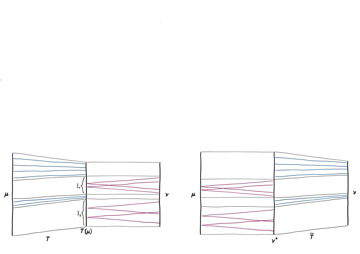 Figure 1
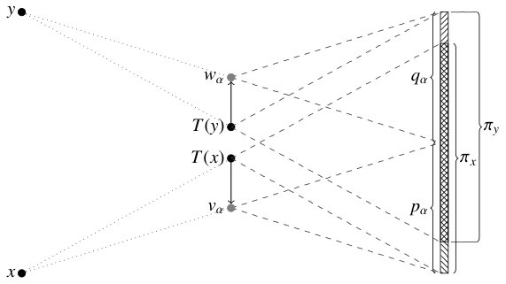 Figure 2
Peer Reviews
No public reviews on file for this paper yet. If you reviewed it on a platform where reviews are public (OpenReview, ICLR, NeurIPS, ICML), you can paste yours below so the community can read it here.
Videos
No videos yet. Explain this paper in a talk, walkthrough, or lecture? Add one.
Weak monotone rearrangement on the line
J. Backhoff-Veraguas
,
M. Beiglböck
and
G. Pammer
Abstract.
Weak optimal transport has been recently introduced by Gozlan et al. The original motivation stems from the theory of geometric inequalities; further applications concern numerics of martingale optimal transport and stability in mathematical finance.
In this note we provide a complete geometric characterization of the weak version of the classical monotone rearrangement between measures on the real line, complementing earlier results of Alfonsi, Corbetta, and Jourdain.
1. Introduction
Recently, there has been a growing interest in weak transport problems as introduced by Gozlan et al [15]. While the original motivation mainly stems from applications to geometric inequalities (cf. the works of Marton [17, 16] and Talagrand [21, 22]), weak transport problems appear also in a number of further topics, including martingale optimal transport [2, 4, 10, 6], the causal transport problem [7, 1], and stability in math. finance [5].
1.1. Framework and main results
Write for the set of couplings between . Starting with the seminal article of Gangbo-McCann [12] problems of the form
[TABLE]
where denotes a convex function have received particular attention in optimal transport. The pendant in weak optimal transport consists in
[TABLE]
Here denotes the convex order, i.e. iff for all convex .
The problem (1.2), and in particular its one dimensional version, is investigated in [2, 15, 14, 19, 18, 20, 11, 13, 8, 5]. The main purpose of this note is to give a complete geometric characterization of the optimizer in one dimension.
Definition 1.1**.**
Fix . We call a function admissible if it satisfies
- (i)
* is increasing,* 2. (ii)
* is 1-Lipschitz,* 3. (iii)
.
Theorem 1.2**.**
Let . There exists an admissible (-a.s. unique) which is maximal in the sense that for every other admissible .
If is convex then is an optimizer of (1.2). If is strictly convex and is finite, is the unique optimizer of (1.2).
We call the (-a.s. unique) map in Theorem 1.2 the weak monotone rearrangement.
A particular consequence of Theorem 1.2 is that the optimizer of (1.2) does not depend on the choice of the convex function . We find this fact non-trivial as well as remarkable and highlight that it is not new: different independent proofs were given by Gozlan et al [15], Alfonsi, Corbetta, Jourdain [2] and Shu [20]. Alfonsi, Corbetta and Jourdain [3, Example 2.4] notice that this does not pertain in higher dimensions.
The map can be explicitly characterized in geometric terms using the notion of irreducibility introduced in [9]: Measures are in convex order iff
[TABLE]
and, by continuity, the set where this inequality is strict is open. Hence , where is an at most countable family of disjoint open intervals; these intervals are called irreducible with respect to .
Theorem 1.3**.**
The weak monotone rearrangement of is the unique admissible map which has slope 1 on each interval , where is irreducible wrt .
Theorem 1.3 represents a necessary and sufficient condition for the optimality of the measure in (1.2). We note that the ‘necessary’ part was first obtained (using somewhat different phrasing) by Alfonsi, Corbetta, and Jourdain [2, Proposition 3.12]. We also refer the reader to the semi-explicit representation of and given in [2].
1.2. Connection with martingale transport plans
Intuitively, the irreducible intervals of are the components where we need to ‘expand’ in order to transform it into . In this sense Theorem 1.3 asserts that the mass of can either concentrate between and , or it can expanded between and (see Figure 1).
To make this precise, we recall from [15] that (1.2) can be reformulated as
[TABLE]
where denotes a regular disintegration of the coupling wrt its first marginal .
The set of optimizers of (1.4) is also straightforward to express in terms of : Write for the set of martingale couplings (or martingale transport plans), i.e. which satisfy barycenter, -a.s. By Strassen’s theorem is nonempty iff . Using this notation, is optimal iff there exists a martingale coupling such that is the concatenation of the transports described by and :
[TABLE]
Any can be decomposed based on the family of irreducible intervals : denoting by [9, Appendix A] we have
[TABLE]
Plainly, (1.6) asserts that any martingale transport plan can move mass only within the individual irreducible intervals, whereas particles have to stay put.
1.3. A reverse problem
Alfonsi, Corbetta, and Jourdain [2] proved that the same value is obtained when reversing the order of transport and convex order relaxation in (1.2), i.e.
[TABLE]
moreover they find ([2, Proposition 3.12]) a monotone mapping which is optimal between the optimizer of (1.7) and as well as between and the optimizer of (1.2).
As a counterpart to Theorems 1.2 and 1.3 we establish the following result, strengthening the connection between (1.2) and (1.7).
Theorem 1.4**.**
Let . Then there exists a unique -smallest measure , , which can be pushed onto by an increasing 1-Lipschitz mapping. Moreover we have
- (1)
If is convex then is an optimizer of (1.7). If is strictly convex and is finite, is the unique optimizer of (1.7). 2. (2)
There exists a (-unique) increasing 1-Lipschitz mapping which pushes onto ; has slope 1 on each interval , where is irreducible wrt . 3. (3)
* is the weak monotone rearrangement between and .*
As in the previous section, (1.7) could be interpreted as a concatenation of a martingale transport with the weak monotone rearrangement.
1.4. An auxiliary result
We close this introductory section which an auxiliary result that will be important in the proofs of our results. Since it might be of independent interest we provide the -dimensional version. We denote the topology induced by the -Wasserstein distance on the space of probability measures on by .
Theorem 1.5** (Stability).**
Let , , and convex and such that for some constant it holds
[TABLE]
If in and in , then . If additionally is strictly convex, we have that
- (1)
, 2. (2)
the sequence of maps , where and , converges in -probability to , where and .
2. C-Monotonicity implies geometric characterization
In this part we prove the following
Theorem 2.1**.**
Let and strictly convex. If yields a finite value, for any optimizer of (1.4), the map
[TABLE]
is -almost surely uniquely defined and is independent of the specific coupling , it is admissible in the sense of Definition 1.1, and it has slope on if is an irreducible interval for .
To prove Theorem 2.1, we need some further properties connected to irreducibility:
Lemma 2.2**.**
Suppose . Then for any , any regular disintegration wrt and any such that , there are , , , such that the supports of and overlap, i.e.
[TABLE]
Proof.
To show this assertion, we assume the opposite. So there exist , with fixed disintegration wrt and
[TABLE]
so that for all with , , we have
[TABLE]
Since is a martingale coupling, and by (2.2), there exists with
[TABLE]
Write for the largest and for the smallest such that (2.3) holds. Note then that . We have either or , which in any case implies . Thus, we infer
[TABLE]
and we conclude by contradicting since
[TABLE]
Lemma 2.3**.**
Let have overlapping supports (cf. (2.1)). Then there exists a continuous map such that
[TABLE]
and such that for some the functions
[TABLE]
are strictly decreasing and increasing, respectively.
Proof.
Let and define the inverse distribution functions by
[TABLE]
where and denote the cumulative distribution functions of and , respectively. Define two auxiliary measures
[TABLE]
Defining probability measures and by and , yields (2.4) and continuity of . Since and satisfy (2.1), we find constants with such that
[TABLE]
Let , then for any we have
[TABLE]
and conclude that for the maps defined in (2.5) are strictly monotone. ∎
An important tool in the proof of Theorem 2.1 is -monotonicity, a concept which was introduced for the weak optimal transport problem in [6, 13, 8].
Definition 2.4** (-monotonicity).**
A coupling is -monotone if there exists a measurable set with , such that for any finite number of points in and measures with
[TABLE]
Proof of Theorem 2.1.
Let be optimal for the weak optimal transport problem (1.4). By the monotonicity principle [8, Theorem 5.2] is -monotone, therefore, there exists a set with and such that for all satisfying we have
[TABLE]
As an immediate consequence, we find that the map is -almost surely increasing. Letting , for any we define
[TABLE]
Plugging and into (2.6) and computing the righthand-side derivative yields
[TABLE]
which is by strict convexity of equivalent to
[TABLE]
Hence, and is -a.e. -Lipschitz.
Further, we have that and . Without loss of generality, we can assume Let be the intervals given by the decomposition of into irreducible intervals. Assume that there is an interval so that on the map does not have -a.s. slope 1. Then Lemma 2.2 provides two points in and two corresponding points such that
[TABLE]
and the overlapping condition (2.1) holds for , . Lemma 2.3 allows us to define measures and on such that
[TABLE]
For a graphical depiction compare with Figure 2. Hence,
[TABLE]
are strictly monotone, continuous maps on . Therefore, we find with
[TABLE]
By strict convexity of we find
[TABLE]
which then yields a contradiction to -monotonicity:
[TABLE]
3. Sufficiency of the geometric characterization
Naturally the question arises whether any map satisfying the properties in Theorem 2.1 must be optimal. The aim of this section is to establish this:
Theorem 3.1**.**
Let . Then any coupling for which is admissible (in the sense of Definition 1.1) with slope on each interval , where is irreducible wrt , is optimal for (1.4), i.e.,
[TABLE]
The proof is based on dual optimizers and their explicit representation. As long as is strictly increasing, [19, Theorem 2.1] provides dual optimizers to . Investigating dual optimizers further, we are able to show here . First, Lemma 3.2 helps us to carefully approximate the increasing map with strictly increasing maps .
Lemma 3.2**.**
Let be an increasing map, with decreasing. Then, for any there is a strictly increasing map , with decreasing, such that
[TABLE]
and is affine with slope on an interval if and only if is affine with slope on .
Proof.
Since is increasing we know that the pre-image of any point under corresponds to an interval. Therefore, we can find at most countable many, disjoint intervals of finite length, where is a singleton and is strictly increasing on the complement, i.e., on . For any , we define
[TABLE]
Then the map satisfies the desired properties. ∎
Let be an increasing 1-Lipschitz function. Then induces a unique decomposition of into at most countably many maximal, closed, disjoint intervals and a (-set) such that for all the map is affine with slope 1 and is properly contractive, i.e., for any two points we have . Below we call the intervals irreducible wrt .
Proof of Theorem 3.1.
The convex function can be approximated by a pointwise-increasing sequence of Lipschitz convex functions , e.g.
[TABLE]
By monotone convergence we find111Recall that by [14] the optimizer of the weak transport problem does not depend on the convex cost. . Indeed, if optimizes and assuming wlog that , then
[TABLE]
by [8, Proposition 2.8]. Thus the claim follows by taking the supremum in .
From this, it suffices to consider the case when is Lipschitz continuous. By Lemma 3.2 we find for any a strictly increasing map , such that is decreasing, the decompositions of and match, and Then [19, Theorem 2.1] provides a convex, Lipschitz continuous function such that for all
[TABLE]
which is even affine on the parts where is affine. Write , where is defined as in (3.1) so . In the following we will show that is a dual optimizer of the coupling defined as the push-forward measure of by the function
[TABLE]
First, we compute the barycenters of :
[TABLE]
and . Given the sets and from the decomposition of into irreducible intervals, we find the sets and from the decomposition of into irreducible intervals by setting
[TABLE]
In view of the structure of martingale couplings, see [9, Theorem A.4], we find that for -a.e. we have and -a.e. on . Since the decompositions of and are complementary, we infer the same for the decompositions of the map and the pair . The next computation establishes duality of the pair , where we use affinity of on the irreducible components of :
[TABLE]
This easily proves that is optimal for the optimal weak transport problem . Drawing the limit for , we observe
[TABLE]
As is Lipschitz, we can apply stability Theorem 1.5 and obtain optimality of . ∎
4. Geometry of the weak monotone rearrangement
We can summarize Theorems 2.1 and 3.1 as follows: There exists an admissible map with slope on whenever is an irreducible interval wrt , such that is optimal for (1.4) iff (-a.s.). We now show that this map is the weak monotone rearrangement and is therefore the maximum in convex order of the set222We abuse terminology here, meaning maximum of .
[TABLE]
Heuristically speaking, if the maximum in convex order of the set is again given by an increasing, 1-Lipschitz map, then this map is as close as possible to a shifted identity. In turn, this is favourable when trying to find the minimum in convex order of
[TABLE]
which gives reason to why there should exist a single optimizer to (1.4) for all convex .
As preparation to establishing Theorem 1.3, we prove Lemma 4.1 and Lemma 4.2.
Lemma 4.1**.**
Let , be increasing maps with
[TABLE]
then the maximum (wrt the convex order) of and , which is uniquely determined by its potential functions, is again given by an increasing map. If in addition, the maps are -Lipschitz with , then the maximum is also given by an -Lipschitz map.
Proof.
The maximum of and wrt. the convex order is uniquely determined by the maximum of its potential functions, i.e. . The right-hand side derivative of the potential function can be expressed by the cumulative distribution function, namely . By continuity of the potential functions, we find a partition of into at most countably many disjoint intervals , where on , and restricted onto one of the following holds true:
- (a)
, 2. (b)
.
Suppose wlog (a) holds, then
[TABLE]
By monotonicity, we can define on 333We use the convention that the maximum of the empty set equals . by
[TABLE]
Hence, is an increasing map, and is given by the map . If and are in addition -Lipschitz, it follows by construction that is -Lipschitz. ∎
Lemma 4.2**.**
Let and , where are increasing and -Lipschitz. Then .
In particular, if and are increasing -Lipschitz maps s.t. , and we denote by the increasing -Lipschitz map with , which exists by Lemma 4.1, then .
Proof.
By approximation, it suffices to settle the case when are uniform measures on atoms. Let denote the atoms of . Then the vector is ordered in an increasing way. What is more, the vector is likewise ordered increasingly, since is an increasing map. By e.g. [14, Proposition 2.6] we know that
[TABLE]
But then also , so again by [14, Proposition 2.6] we conclude . The second statement easily follows from the first one. ∎
Proof of Theorem 1.3.
Existence of an admissible map which has slope 1 on each interval , where is irreducible wrt , was already shown in Theorem 2.1. Therefore, it remains to show that the map is maximal. Denote by the map given by Theorem 2.1 associated with an optimizer to (1.4) and some strictly convex . Let be an arbitrary map in . Then Lemma 4.2 states that
[TABLE]
where is defined as the increasing, 1-Lipschitz map such that . Additionally to existence, strict convexity of ensures -almost sure uniqueness of in the sense that for any optimal coupling we have Thus, and -almost surely. ∎
Proof of Theorem 1.2.
This is a direct consequence of Theorem 2.1, which provides existence of a map with the desired geometric properties, and Theorem 1.3, which provides the equivalence between the geometric properties and maximality. ∎
5. On the reverse problem of Alfonsi, Corbetta, and Jourdain
We aim to prove Theorem 1.4 pertaining the reverse problem (1.7).
Lemma 5.1**.**
Let , be increasing maps with
[TABLE]
Denote the minimum in convex order of and by . Then there exists an increasing map such that . If in addition, the maps are -Lipschitz with , then the same holds true for .
Proof.
Suppose there exist increasing maps and measures , , such that . Then the potential function of the minimum of and wrt the convex order is given by the convex hull of and . The potential function completely specifies the cumulative distribution function through . Thus, we can find a partition of into countably many, disjoint intervals . For each , we have with , such that one of the following holds
- (a)
on , 2. (b)
and on .
According to this decomposition, we can define an increasing map via
[TABLE]
Note that is -Lipschitz if , , are -Lipschitz. Let , due to the continuity of the maps and , we can find points with , . Assume that with . If (a) holds, then we have . Now presume that (b) holds, then . Then
[TABLE]
Hence, by monotonicity of the map we conclude . ∎
Proof of Theorem 1.4.
Define via the weak monotone rearrangement between and , as on the contraction parts of and accordingly shifted on the affine (irreducible) intervals such that . Let . Then for any strictly convex and coupling we have with equality iff is actually given by a map. Hence, if the optimizer of is not given by a map and , we have
[TABLE]
Thus, by the structure of the weak monotone rearrangement, we deduce optimality of for Problem (1.7). To show uniqueness of (1.7), assume that attains the minimum of (1.7) and the optimizer of is given by the map . For any martingale coupling we define a map by
[TABLE]
Then by optimality and, in particular,
[TABLE]
which shows -almost surely. By strict convexity, we have
[TABLE]
Since was arbitrary in we get that is affine with slope on , whenever is an irreducible interval wrt . Therefore and restricted to coincide. Hence, .
We finally show that is minimal in the convex order as stated. By Lemma 5.1, we can assume and that can be pushed forward onto via an increasing -Lipschitz map . It follows by Lemma 4.2 that , so
[TABLE]
and by the uniqueness obtained above we deduce . ∎
6. Stability of barycentric weak transport problems in multiple dimensions
The final part of the article is concerned with stability of the weak optimal transport problem under barycentric costs, see (1.4). Unlike in the rest of the article we work here on . The final aim is to prove Theorem 1.5.
One surprising aspect of this result is that we only require in and not necessarily in . This relates to the conditional expectation in (1.4) being ‘inside of .’ We first prove an illuminating intermediate result:
Proposition 6.1**.**
Let , , and convex and satisfying the growth condition (1.8). Suppose that and in , and that . Then there exist such that
- (i)
* in ,*
- (ii)
**
Proof.
It is well-known that together with the stated convergence of the ’s implies , so we proceed to prove the former. Let be an optimal coupling attaining . Let be any martingale coupling with first marginal and second marginal , the existence of which is guaranteed by the assumption together with Strassen’s theorem. We convene on the notation and , and define the measure
[TABLE]
This measure has , and as first, second and third marginals. We next define as the conditional expectation under of the third variable given the first one, namely
[TABLE]
Next we introduce so by definition . Finally
[TABLE]
by the martingale property and two applications of Jensen’s inequality. The desired conclusion follows. ∎
Remark 6.2*.*
In the context of the previous proposition, if is supported in finitely many atoms, then the condition that in can be relaxed to convergence in . To wit, if , one can take in (6.1) and prove
[TABLE]
so taking -power and integrating w.r.t. we get .
The previous remark shows that we need to reduce to the finite-support setting. We carry to this in the next two lemmas:
Lemma 6.3**.**
Let . Then for any there is a compactly supported, positive measures with
[TABLE]
Proof.
We first partition into countable, disjoint -dimensional cubes of length . Define an approximation of by
[TABLE]
Note that and in when . If there exists an approximation such that the assertion holds, then it is straightforward to construct the corresponding measure for , which in turn satisfies the assertion with respect to . Wlog, we may assume that
[TABLE]
where denotes the barycenter of . Then we can find such that
[TABLE]
Let span in the sense above and
[TABLE]
For any there is a such that
[TABLE]
Besides, there exists a compact set such that
[TABLE]
and . Therefore, we find with
[TABLE]
If is chosen smaller than for all , we can define the via
[TABLE]
Lemma 6.4**.**
Let and convex satisfying the growth condition (1.8). Then there exists a sequence of finitely supported measures with , in and .
Proof.
For any we find a compact set such that . For any , the set can be covered by finitely many, disjoint sets with diameter smaller than and . Define the measure by
[TABLE]
where the points and are given by
[TABLE]
By construction, there exists a martingale coupling between and , thus, . Note that restricted to is Lipschitz continuous. Then drawing the limit yields
[TABLE]
and by convexity, Choosing sufficiently small, we have
[TABLE]
By the growth condition (1.8) and stability, we obtain . ∎
We can now prove a version of Proposition 6.1 under weaker assumptions:
Lemma 6.5**.**
Let be a sequence in and let be a sequence with in , in , where , and let be a convex functions satisfying the growth constraint (1.8). Then for any we find a sequence of such that and in .
Proof.
Wlog assume that is positive. By Lemma 6.3, we can find for any a compactly supported with , and
[TABLE]
where . Using stability of classical optimal transport, see [23, Theorem 5.20], we may assume that . By Lemma 6.4 we may reduce to the case of finitely supported . We conclude the proof with Remark 6.2. ∎
Finally we can give the pending proof of Theorem 1.5:
Proof of Theorem 1.5.
Lower-semicontinuity of the map follows from [8, Theorem 1.3]. By [8, Lemma 6.1] we have
[TABLE]
where the infimum is even attained for a measure . By Lemma 6.5 we find a sequence , so that again using [8, Lemma 6.1] we find
[TABLE]
If is strictly convex, the infimum in (6.4) is attained by a unique probability measure ,444The uniqueness of , and was already shown in [2, Theorem 2.1] for , which in turn is the push-forward of under a -uniquely defined map . Moreover, the -optimal transport plan is uniquely determined by : Suppose the contrary and let , then and we find the contradiction
[TABLE]
Hence, by convergence of the values of and tightness of , we deduce the convergence of the to the optimal in . Suppose that for all , then due to the uniqueness of the optimal transport maps between and ), we can apply Theorem [23, Corollary 5.23] and obtain convergence of the transport maps to . ∎
The reference list from the paper itself. Each links out to its DOI / PubMed record.
- 1[1] B. Acciaio, J. Backhoff-Veraguas, and A. Zalashko. Causal optimal transport and its links to enlargement of filtrations and continuous-time stochastic optimization. Ar Xiv e-prints , 2016.
- 2[2] A. Alfonsi, J. Corbetta, and B. Jourdain. Sampling of probability measures in the convex order and approximation of Martingale Optimal Transport problems. Ar Xiv e-prints , Sept. 2017.
- 3[3] A. Alfonsi, J. Corbetta, and B. Jourdain. Sampling of probability measures in the convex order by Wasserstein projection. ar Xiv e-prints , page ar Xiv:1709.05287, Feb. 2019.
- 4[4] J.-J. Alibert, G. Bouchitte, and T. Champion. A new class of cost for optimal transport planning. hal-preprint , 2018.
- 5[5] J. Backhoff-Veraguas, D. Bartl, M. Beiglböck, and M. Eder. Adapted wasserstein distances and stability in mathematical finance. Ar Xiv e-prints , 2019.
- 6[6] J. Backhoff-Veraguas, M. Beiglböck, M. Huesmann, and S. Källblad. Martingale Benamou–Brenier: a probabilistic perspective. Ar Xiv e-prints , Aug. 2017.
- 7[7] J. Backhoff-Veraguas, M. Beiglböck, Y. Lin, and A. Zalashko. Causal transport in discrete time and applications. SIAM Journal on Optimization , 27(4):2528–2562, 2017.
- 8[8] J. Backhoff-Veraguas, M. Beiglböck, and G. Pammer. Existence, duality, and cyclical monotonicity for weak transport costs. Ar Xiv e-prints , 2018.