A New Smoothing Technique based on the Parallel Concatenation of Forward/Backward Bayesian Filters: Turbo Smoothing
Giorgio M. Vitetta, Pasquale Di Viesti, Emilio Sirignano

TL;DR
This paper introduces turbo smoothing, a new method combining forward and backward Bayesian filters via parallel concatenation, improving complexity-accuracy tradeoff in smoothing for linear Gaussian systems.
Contribution
It extends turbo filtering concepts to smoothing, proposing algorithms that outperform recent methods in complexity and accuracy for certain systems.
Findings
Achieves better complexity-accuracy tradeoff
Demonstrates improved performance over recent smoothing techniques
Validates algorithms with numerical results on linear Gaussian systems
Abstract
Recently, a novel method for developing filtering algorithms, based on the parallel concatenation of Bayesian filters and called turbo filtering, has been proposed. In this manuscript we show how the same conceptual approach can be exploited to devise a new smoothing method, called turbo smoothing. A turbo smoother combines a turbo filter, employed in its forward pass, with the parallel concatenation of two backward information filters used in its backward pass. As a specific application of our general theory, a detailed derivation of two turbo smoothing algorithms for conditionally linear Gaussian systems is illustrated. Numerical results for a specific dynamic system evidence that these algorithms can achieve a better complexity-accuracy tradeoff than other smoothing techniques recently appeared in the literature.
Click any figure to enlarge with its caption.
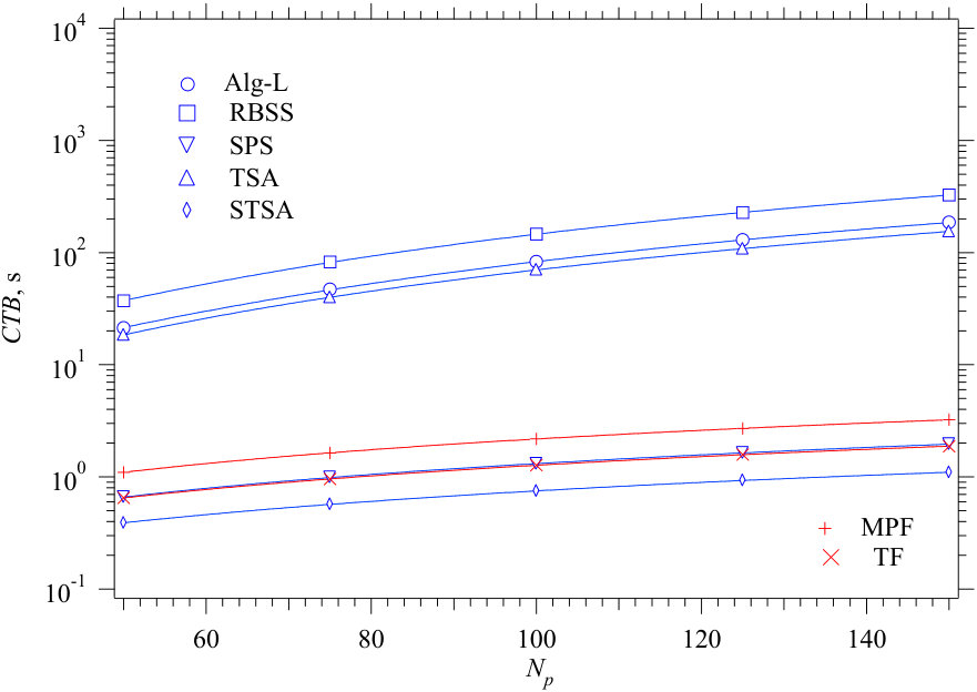 Figure 1
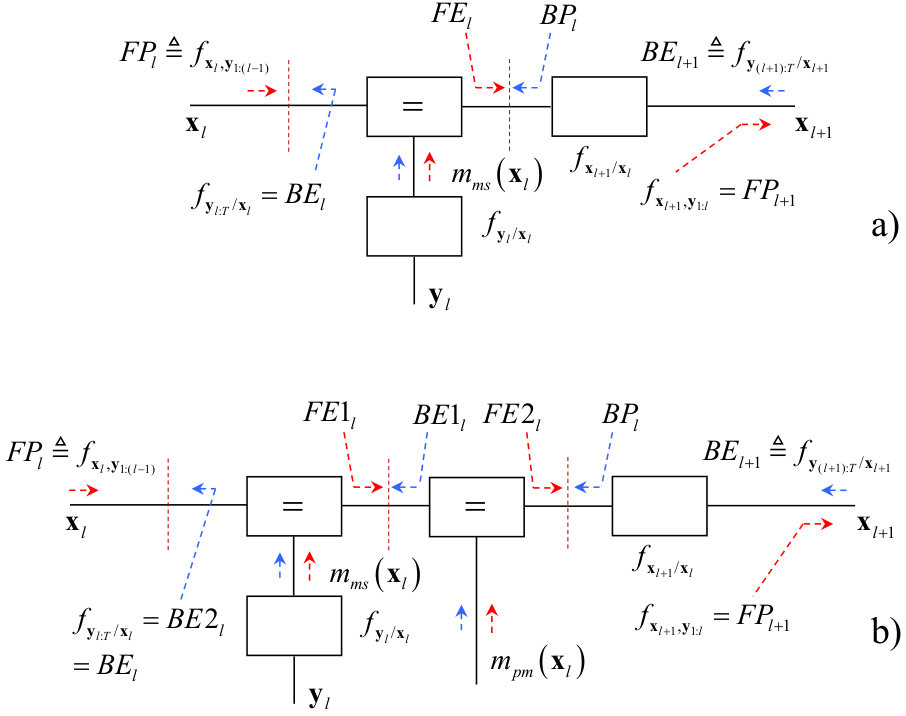 Figure 1
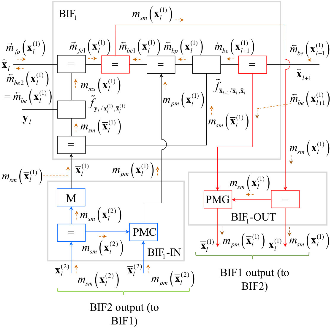 Figure 2
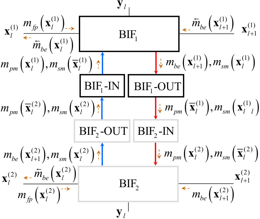 Figure 3
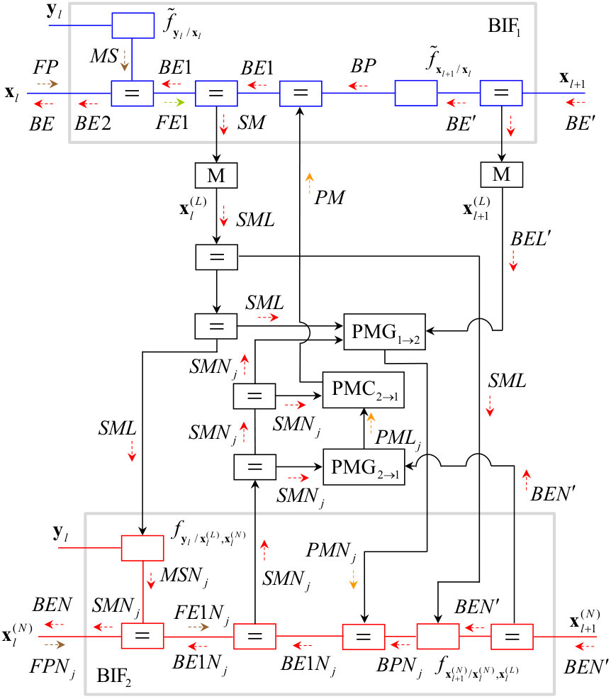 Figure 4
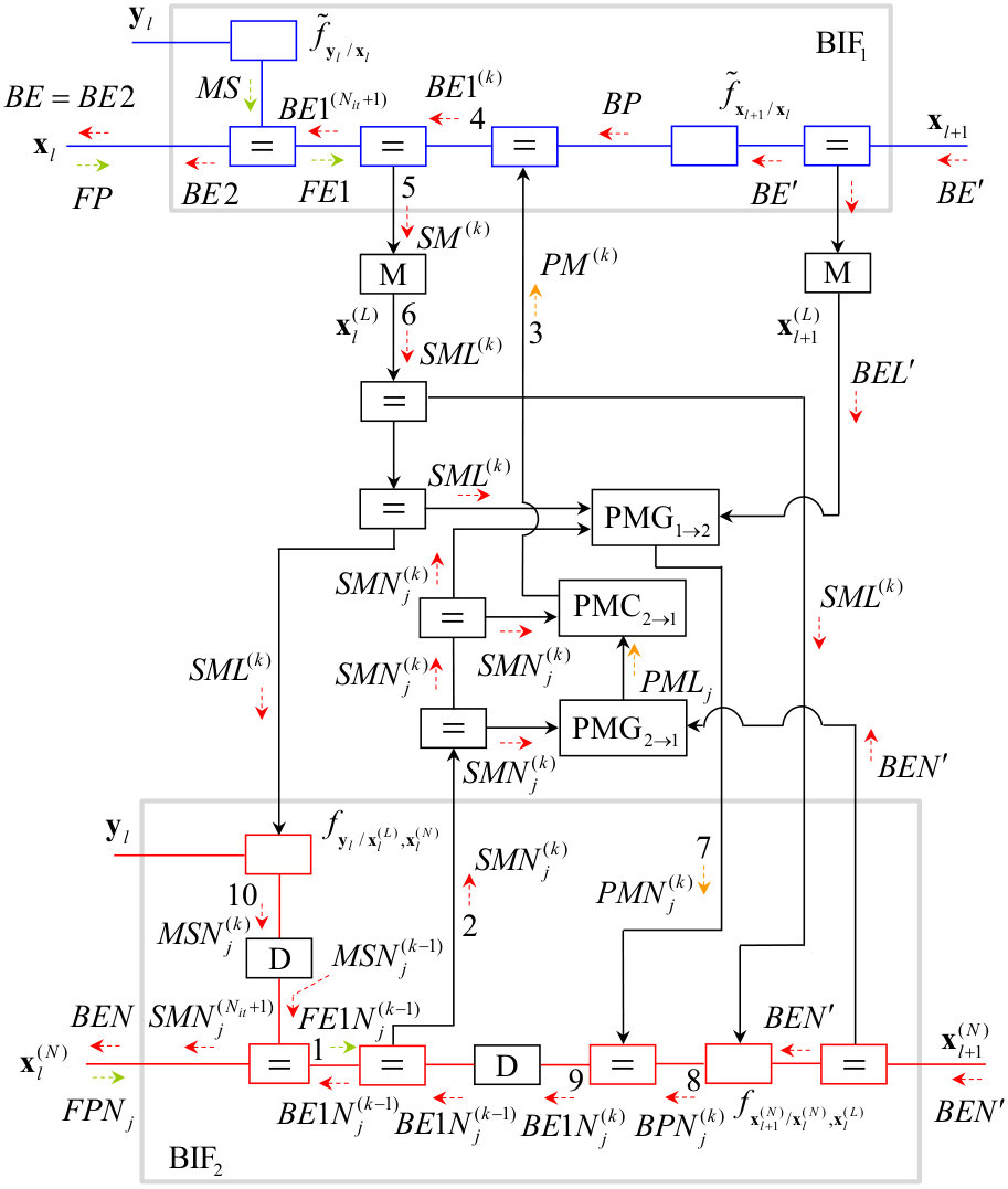 Figure 5
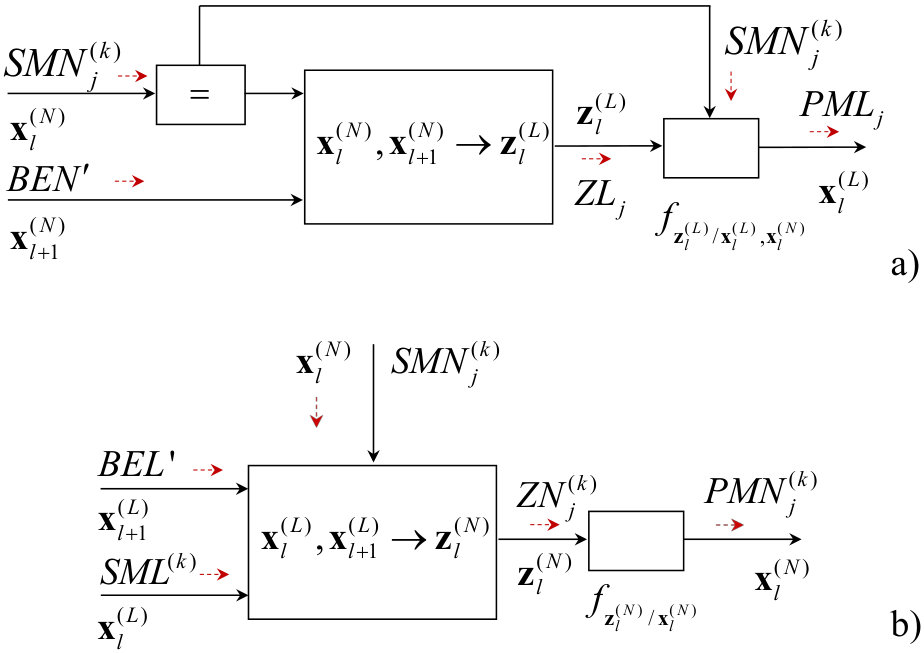 Figure 7
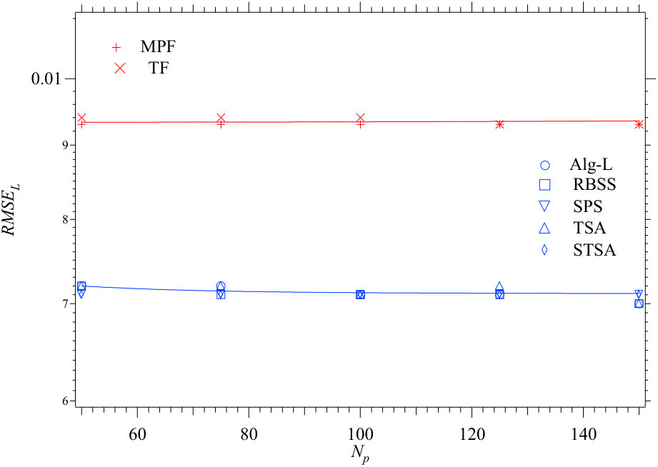 Figure 8
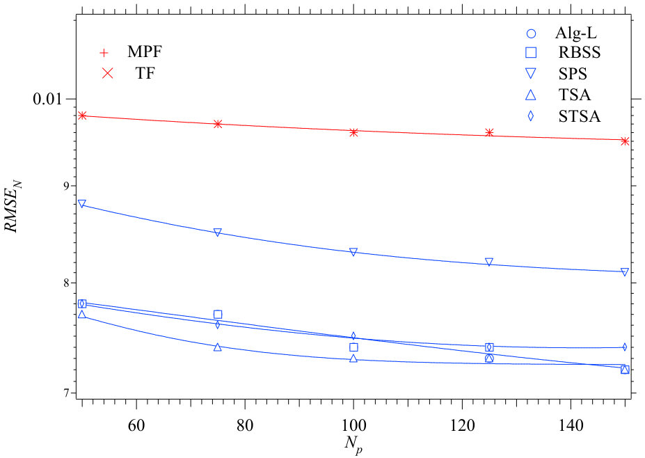 Figure 9
Peer Reviews
No public reviews on file for this paper yet. If you reviewed it on a platform where reviews are public (OpenReview, ICLR, NeurIPS, ICML), you can paste yours below so the community can read it here.
Videos
No videos yet. Explain this paper in a talk, walkthrough, or lecture? Add one.
Taxonomy
TopicsTarget Tracking and Data Fusion in Sensor Networks · Gaussian Processes and Bayesian Inference · Bayesian Modeling and Causal Inference
A New Smoothing Technique based on the Parallel Concatenation of
Forward/Backward Bayesian Filters: Turbo Smoothing
Abstract
Recently, a novel method for developing filtering algorithms, based on the parallel concatenation of Bayesian filters and called turbo filtering, has been proposed. In this manuscript we show how the same conceptual approach can be exploited to devise a new smoothing method, called turbo smoothing. A turbo smoother combines a turbo filter, employed in its forward pass, with the parallel concatenation of two backward information filters used in its backward pass. As a specific application of our general theory, a detailed derivation of two turbo smoothing algorithms for conditionally linear Gaussian systems is illustrated. Numerical results for a specific dynamic system evidence that these algorithms can achieve a better complexity-accuracy tradeoff than other smoothing techniques recently appeared in the literature.
Giorgio M. Vitetta, Pasquale Di Viesti and Emilio Sirignano
University of Modena and Reggio Emilia
Department of Engineering ”Enzo Ferrari”
Via P. Vivarelli 10/1, 41125 Modena - Italy
email: [email protected], [email protected], [email protected]
Keywords: Hidden Markov Model, Smoothing, Factor Graph, Particle Filter, Kalman Filter, Parallel Concatenation, Sum-Product Algorithm, Turbo Processing.
1 Introduction
The problem of Bayesian smoothing for a state space model (SSM) concerns the development of recursive algorithms able to estimate the probability density function (pdf) of the model state on a given observation interval, given a batch of noisy measurements acquired over it [1]; the estimated pdf is known as a smoothed or smoothing pdf. A general strategy for solving this problem is based on the so called two-filter smoothing formula [2]-[3]; in fact, this formula allows to compute the required smoothing density by merging the statistical information generated in the forward pass of a Bayesian filtering method with those evaluated in the backward pass of a different filtering method, paired with the first one and known as backward information filtering (BIF). Unluckily, closed form solutions for this strategy can be derived for linear Gaussian and linear Gaussian mixture models only [1], [4]. For this reason, all the existing smoothing algorithms based on the above mentioned formula and applicable to general nonlinear models are approximate and are based on sequential Monte Carlo techniques (e.g., see [2], [5], [6] and references therein). Unluckily, the adoption of these algorithms, known as particle smoothers, may be hindered by their complexity, which becomes unmanageable when the dimension of the sample space for the considered SSM is large.
Recently, a factor graph approach has been exploited to devise a new filtering method, based on the parallel concatenation of two (constituent) Bayesian filters and called *turbo filtering *(TF) [7]. In this manuscript, a new smoothing technique that employs TF in its forward pass and a new BIF scheme, based on the parallel concatenation of two backward information filters, is developed. Our derivation of the new BIF method, called backward information turbo filtering (BITF), is based on a general graphical model; this allows us to: a) represent any BITF algorithm as the interconnection of *two soft-in soft-out *(SISO) processing modules; b) represent the iterative processing accomplished by these modules as a message passing technique; c) derive the expressions of the passed messages by applying the sum-product algorithm (SPA) [8], [9], together with a specific scheduling procedure, to the graphical model itself; d) show how the statistical information generated by a BITF algorithm in the backward pass can be merged with those produced by the paired TF technique in the forward pass in order to evaluate the required smoothed pdfs. To exemplify the usefulness of this smoothing method, called turbo-smoothing (TS) in the following, we take into consideration the TF algorithms proposed in [7] for the class of conditionally linear Gaussian (CLG) SSMs and derive a BITF algorithm paired with them. This approach leads to the development of two new TS algorithms, one generating an estimate of the joint smoothing density over the whole observation interval, the other one an estimate of the marginal smoothing densities over the same interval. Our computer simulations for a specific CLG SSM evidence that, in the considered case, the derived TS algorithms perform very closely to the Rao-Blackwellized particle smoothing (RBPS) technique proposed in [10] and to the particle smoothers devised in [11].
The remaining part of this manuscript is organized as follows. A description of the considered SSMs is illustrated in Section 2. In Section 3, a general graphical model on which the processing accomplished in BITF and TS is based is illustrated; then, a specific instance of it, referring to a CLG SSM, is developed and the messages passed over it in BITF are defined. In Section 4, the scheduling and the computation of such messages are described, specific TS algorithms are developed, and the differences and similarities between these algorithms and other smoothing techniques are briefly analysed. A comparison, in terms of accuracy and execution time, between the proposed techniques and three smoothers recently appeared in the literature is provided in Section 5 for a specific CLG SSM. Finally, some conclusions are offered in Section 6.
Notations: The same notations as refs. [11], [7] and [12] are adopted.
2 Model Description
In this manuscript we focus on a discrete-time SSM whose -dimensional hidden state in the -th interval is denoted , and whose state update and measurement models are expressed by
[TABLE]
and
[TABLE]
respectively. Here, () is a time-varying -dimensional (-dimensional) real function and () the -th element of the process (measurement) noise sequence (); this sequence consists of -dimensional (-dimensional) independent and identically distributed (iid) Gaussian noise vectors, each characterized by a zero mean and a covariance matrix (). Moreover, statistical independence between and is assumed.
In the following, two additional mathematical representations for the considered SSM are also exploited. The first one is approximate, being employed by an extended Kalman filter (EKF); in fact, it is based on the linearized versions of eqs. (1) and (2), namely (e.g., see [1, pp. 194-195])
[TABLE]
and
[TABLE]
respectively; here, , is the (forward) estimate of evaluated by the EKF in its -th recursion, , , is the (forward) prediction computed by the EKF in its -th recursion and .
The second representation is based on the additional assumption that the SSM described by eqs. (1)-(2) is CLG [10], [13], so that its state vector in the -th interval can be partitioned as ; here, , () is the so called *linear *(nonlinear) component of , with (). For this reason, following [11], [12] and [13], the models
[TABLE]
and
[TABLE]
are adopted for the update of the linear () and nonlinear () components and for the measurement vector, respectively. In the state update model (5), () is a time-varying -dimensional real function ( real matrix) and consists of the first (last ) elements of if (); independence between and is also assumed for simplicity and the covariance matrix () is denoted (). In the measurement model (6), instead, () is a time-varying -dimensional real function ( real matrix).
In the next two Sections we focus on the problem of developing algorithms for the estimation of a) the joint smoothed pdf (problem P.1) and b) the sequence of marginal *smoothed pdfs * (problem P.2); here, is the duration of the observation interval and is a -dimensional vector. It is important to point out that: a) in solving both problems P.1 and P.2, the prior knowledge of the pdf of the initial state is assumed; b) in principle, if an estimate of the joint pdf is available, estimates of all the posterior can be evaluated by marginalization.
3 Graphical Modelling for the Parallel Concatenation of Bayesian
Information Filters
In this Section, we derive the graphical models on which BITF and TS techniques are based. More specifically, starting from the factor graph representing Bayesian smoothing [11], we first develop a general graphical model for the parallel concatenation of two backward information filters. Then, a specific instance of this model is devised for the case in which the forward filters are an EKF and a particle filter (PF), and the considered SSM is CLG.
3.1 Graphical Model for the Parallel Concatenation of Bayesian
Information Filters and Message Passing over it
The development of our BIF algorithms is based on the graphical approach illustrated in ref. [11, Sec. III]. This approach consists in representing Bayesian filtering and BIF as two recursive algorithms that compute, on the basis of the SPA, a set of probabilistic messages passed along the same (cycle free) factor graph; this graph is illustrated Fig. 1-a) and refers to a SSM characterized by the Markov model and the measurement model . More specifically, in the -th recursion of Bayesian filtering*, *messages are passed along the considered graph in the forward direction; moreover, the messages and (denoted and , respectively, in Fig. 1 and conveying a forward estimate of and a forward prediction of , respectively) are computed on the basis of the input message
[TABLE]
for , , , (). Dually, in the -th recursion of BIF, messages are passed along the considered graph in the backward direction, and the messages and (denoted and , respectively, in Fig. 1 and conveying a backward prediction of and a backward estimate of , respectively) are computed on the basis of the input message
[TABLE]
with (). Once the backward pass is over, a solution to problem P.2 becomes available, since the marginal smoothed pdf can be evaluated as111Note that, similarly as [11] and [12], the joint pdf is considered here in place of the posterior pdf .
[TABLE]
or, equivalently, as
[TABLE]
with . Note that, from a graphical viewpoint, formulas (9) and (10) can be related with the two different partitionings of the graph shown in Fig. 1-a) (where a specific partitioning is identified by a brown dashed vertical line cutting the graph in two parts).
In ref. [7] it has been also shown that the factor graph illustrated in Fig. 1-a) can be employed as a building block in the development of a larger graphical model that represents a turbo filtering scheme, i.e. the parallel concatenation of two (constituent) Bayesian filters (denoted F1 and F2 in the following). In this model, the graphs referring to F1 and F2 are interconnected in order to allow the mutual exchange of statistical information in the form of pseudo-measurements (conveyed by probabilistic messages). From a graphical viewpoint, the exploitation of these additional information in each filter requires:
a) modifying the graph shown in Fig. 1-a) in a way that each constituent filter can benefit from the pseudo-measurements provided by the other filter through an additional measurement update;
b) developing message passing algorithms over a proper graphical model for
- the conversion of the statistical information generated by each constituent filter into a form useful to the other one and 2) the generation, inside each constituent filter, of the statistical information to be made available to the other filter.
As far as the need expressed at point a) is concerned, the graph of Fig. 1-a) can be easily modified by adding a new equality node and a new edge along which the message , conveying pseudo-measurement information, is passed; this results in the factor graph shown in Fig. 1-b). Note that, in the new graphical model, two forward estimates (backward estimates) are computed in the forward (backward) pass. The first estimate, represented by () is generated by merging () with the message () conveying measurement (pseudo-measurement) information, whereas the second one, represented by (), is evaluated by merging () with the message (). Moreover, similarly as the previous case, the smoothed pdf can be computed as
[TABLE]
note also that each of these factorisations can be associated with one of the three distinct vertical cuts drawn in Fig. 1-b).
As far as point b) is concerned, in ref. [7] it is shown that, in any TF scheme, all the processing tasks related to the conversion (generation) of the statistical information emerging from (feeding) each constituent filter can be easily incorporated in a single* module*, called soft-in soft-out (SISO) module and whose overall processing can be represented as message passing over a graphical model including the factor graph shown in Fig. 1-b). For this reason, any TF scheme can be devised by linking (i.e., by concatenating) two SISO modules, each incorporating a specific filtering algorithm and exchanging probabilistic information in an iterative fashion. It is also important to point out that the two constituent filters are not required to estimate the whole system state. For this reason, in the following, we assume that: a) the filter Fi estimates the portion (with and ) of the state vector (the size of is denoted , with ); b) the portion of not included in is denoted , so that the equalities or hold. However, the vector () is required to be part of (or, at most, to coincide with) (), so that an overall estimate of the system state can be always generated on the basis of the posterior pdfs of and evaluated by F1 and F2, respectively. In fact, this constraint on and leads to the conclusion that, generally speaking, the portion of , collecting state variables, is estimated by both F1 and F2, being shared by and .
A similar conceptual approach is followed in the remaining part of this Paragraph to derive the general representation of the BIF technique paired with a given TF scheme, that is, briefly, a backward information turbo filtering (BITF) technique. This means that:
-
The general architecture we propose for BITF is based on the parallel concatenation of two constituent Bayesian information filters, that are denoted BIF1 and BIF2 in the following.
-
The processing accomplished by BIF1 (BIF2) is represented as a message passing algorithm over the same graphical model as F1 (F2).
-
BITF processing can be represented as the iterative exchange of probabilistic information between two distinct SISO modules.
-
The -th SISO module (with and ) incorporates a specific BIF algorithm, that can be represented as a message passing over a factor graph similar to that shown in Fig. 1-b) and that estimates the portion of .
The graphical model developed for the SISO module based on BIF1 is shown in Fig. 2. In this Figure, to ease the interpretation of message passing, three rectangles, labeled as BIF1-IN, BIF1 and BIF1-OUT, have been drawn; this allow us to easily identify the portions of the graphical model involved in a) the conversion of the statistical information provided from BIF2 into a form useful to BIF1, b) BIF1 processing and c) the generation of the statistical information made available by BIF1 to BIF2, respectively. A detailed description of the signal processing tasks accomplished within each portion is provided below.
BIF1-IN - The statistical information provided by BIF2 to the considered SISO module is condensed in the messages and ; these convey a smoothed estimate of and pseudo-measurement information about , respectively. The first message is processed in two different ways. In fact, on the one hand, it is marginalised in the block labelled by the letter M (see Fig. 2) in order to generate the pdf (do not forget that the state vector is included in ); on the other hand, is processed jointly with in order to generate the message conveying pseudo-measurement information about (this is accomplished in the block called PM* conversion*, PMC; see Fig. 2). Then, the messages and are passed to BIF1.
BIF1 - The message passing accomplished in this part refers to the BIF algorithm paired with F1. The graphical model developed for it and the message passing accomplished over it are based on Fig. 1-b). Note, however, that: a) the message passing aims at computing the (backward) predicted density and the (backward) filtered density and on the basis of the backward estimate originating from the previous recursion, and of the messages and provided by BIF1-IN; b) an approximate model of the considered SSM could be adopted in the evaluation of these densities. For this reason, generally speaking, we can assume that the BIF1 algorithm is based on the Markov model and on the observation model , representing the exact models and , respectively, or approximations of one or both of them. Note also that, in both the second measurement update and the time update accomplished by this algorithm, marginalization with respect to the unknown state component is made possible by the availability of the message .
BIF1-OUT - This part is fed by the backward estimate of and by the smoothed estimate of (available after that the first measurement update has been accomplished by F1). The second message follows two different paths, since a) it is passed to the other SISO module as it is and b) it is jointly processed with in order to generate the pseudo-measurement message feeding the other SISO module; the last task is accomplished in the pseudo-measurement generation (PMG) block.
A graphical model structurally identical to the one shown in Fig. 2 can be easily drawn for the SISO module based on BIF2 by interchanging () with (). Merging the graphical model shown in Fig. 2 with its counterpart referring to BIF2 results in the parallel concatenation architecture illustrated in Fig. 3 (details about the underlying graphical model are omitted for simplicity) and on which TS is based. It is important to point out that:
-
The overall graphical model derived for TS, unlike the one illustrated in Fig. 1, is not cycle free; therefore, the application of the SPA to it requires defining a proper message scheduling and, generally speaking, results in iterative algorithms.
-
At the end of the -th recursion of a TS algorithm, two smoothed densities, namely and , are available. This raises the problem of how these statistical information can be fused in order to get a single pdf for (and, in particular, a single smoothed estimate of) the -dimensional portion of estimated by both F1/BIF1 and F2/BIF2. Unluckily, this remains an open issue. In our computer simulations, a simple selection strategy has been adopted in state estimation, since one of the two smoothed estimates of has been systematically discarded.
3.2 A Graphical Model for the Parallel Concatenation of the Bayesian
Information Filters Paired with an Extended Kalman Filter and a Particle Filter
In the remaining part of this manuscript we focus on a specific instance of the proposed TS architecture, since we make the same specific choices as [7] for both the SSM and the filters employed in the forward pass. In particular, we focus on the CLG SSM described in Section 2 and assume that:
-
BIF1 is the backward filter associated with an EKF operating over the whole system state (so that and is empty). In other words, BIF1 is a backward Kalman filter based on a linearised model of the considered SSM.
-
BIF2 is a backward filter associated with a PF (in particular, a sequential importance resampling filter [14]) operating on the nonlinear state component only (so that and ) and representing it through a set of particles (note that elements of the system state are shared by the two BIF algorithms). This means that BIF2 is employed to compute new weights for all the elements of the particle set generated by the PF in the forward pass.
Based on the general models shown in Figs. 2 and 3, the specific graphical model illustrated in Fig. 4 (and referring to the -th recursion of backward filtering) can be drawn for the considered case. In the following, we provide various details about the adopted notation and the message passing within each constituent filter and from each filter to the other one.
Message passing within BIF1 - BIF1 is based on the approximate statistical models and ; these are derived from the linearised eqs. (3) and (4), respectively. Moreover, the (Gaussian) messages passed over its graph (enclosed within the upper rectangle appearing in Fig. 4) are , , , , , (), and , and are denoted , , , , , (), and , respectively, to ease reading.
Message passing within BIF2 - BIF2 is based on the exact statistical models , and , that are derived from the eqs. (5) (with ) and (6), respectively. Moreover, the messages processed by it and appearing in Fig. 4 refer to the -th particle predicted in the previous (i.e., in the -th) recursion of forward filtering and denoted , with ; such messages are , , , , , , and , and are denoted , , , , , , and , respectively, to ease reading.
Message passing from BIF1 to BIF2 - BIF2 is fed by the message and the message set conveying pseudo-measurement information; these messages are computed on the basis of the statistical information made available by BIF1. More specifically, on the one hand, the message (denoted ) results from the marginalization of and is employed for marginalising the PF state update and measurement models (i.e., , and , respectively) with respect to . On the other hand, the pseudo-measurement message (denoted ) is evaluated in the PMG1→2 block by processing the messages and (denoted and resulting from the marginalization of ), under the assumption that is represented by the -th particle (conveyed by the message ).
As illustrated in the Appendix, the computation of the message involves the evaluation of the pdf of the random vector
[TABLE]
defined on the basis of the state update equation (5) (with ) and conditioned on the fact that . This pdf, which is computed according to the joint statistical characterization of and provided by BIF1, is conveyed by the message (not appearing in Fig. 4). Note also that from eq. (5) (with ) the equality
[TABLE]
is easily inferred; the pdf of evaluated on the basis of the right-hand side (RHS) of eq. (15) is denoted in the following.
Message passing from BIF2 to BIF1 - BIF1 is fed by the message that, unlike the set passed to BIF2, provides pseudo-measurement information about the whole state . This message is generated as follows. The message set produced by the PF is processed in the PMG2→1 block, that computes the set of pseudo-measurement messages referring to the linear state component only. Then, the two sets and are merged in the PMC2→1 block, where the information they convey are converted into the (single) message . Moreover, as illustrated in the Appendix, the message conveys a sample of the random vector [13]
[TABLE]
such a sample is generated under the assumption that . The pdf of the random vector is evaluated on the basis of the joint statistical representation of the couple , produced by BIF2 and is conveyed by the message (not appearing in Fig. 4); note also that from eq. (5) (with ) the equality
[TABLE]
is easily inferred; the pdf of evaluated on the basis of the RHS of eq. (17) is denoted in the following.
The rationale behind the message passing illustrated above can be summarized as follows. The message is extracted from the statistical information generated by BIF2 and is exploited by BIF1 to refine its backward estimate of the whole state; moreover, merging this estimate with the forward estimate allows to generate a more accurate statistical representation for and, consequently, for (these are conveyed by and , respectively); finally, these statistical information are exploited to aid BIF2 in the computation of more refined weights of the particles representing .
Given the graphical model shown in Fig. 4 and the messages passed over it, the derivation of a specific BITF algorithm requires: a) defining the mathematical structure of the input messages that feed the -th recursion of backward filtering and that of the output messages emerging from both backward filtering and smoothing in the same recursion; b) describing message scheduling; c) deriving mathematical expressions for all the computed messages. These issues are analysed in detail in Section 4.
4 Scheduling and Computation of Probabilistic Messages in Turbo
Smoothing Algorithms for CLG Models
In this Section, the specific issues raised at the end of the previous Section and concerning the message passing accomplished over the graphical model shown in Fig. 4 are addressed. For this reason, we first provide various details about a) the messages feeding backward filtering, and b) the messages emerging from it and from the related smoothing. Then, we focus on the scheduling of such messages and on their computation. This allows us to develop two new smoothing techniques, one solving problem P.1, the other one problem P.2. Finally, these techniques are briefly compared with other particle smoothing methods available in the literature.
4.1 Input and Output Messages
The input messages feeding the -th recursion of backward filtering are generated in the -th recursion of the paired forward filtering and in the previous recursion (i.e., in the -th recursion) of the backward pass. In the following, various details about such messages are provided.
- Input messages evaluated in the forward pass - A turbo filter, consisting of an EKF (denoted F1) and a PF (denoted F2), is employed in the forward pass of the devised TS algorithms and is run only once. Therefore, the forward predictions/estimates, provided by F1 (F2) and made available to BIF1 (BIF2), are expressed by Gaussian pdfs (sets of weighted particles), each conveyed by a Gaussian message (by a set of particle-dependent messages). The notation adopted in the following for these probabilistic information is summarized below.
Filter F1 - This filter, in its -th recursion, computes the forward prediction of , conveyed by the message222Considerations similar to the ones expressed for (18) and (19) can be repeated for the messages (22) and (23), respectively, defined below. (see Fig. 4)
[TABLE]
This message is updated in the -th recursion of F1 on the basis of the measurement . This produces the Gaussian message
[TABLE]
representing a forward estimate of ; the covariance matrix and the mean vector can be evaluated on the basis of the associated precision matrix (see [11, eqs. (14)-(17)])
[TABLE]
and of the transformed mean vector
[TABLE]
respectively; here, , and . The message (18) enters the graphical model developed for BIF1 (see Fig. 4) along the half edge referring to .
Filter F2 - This filter, in its -th recursion, computes the particle set , representing a forward prediction of ; the weight assigned to the particle is equal to for any , since the use of particle resampling in each recursion is assumed. The statistical information available about are conveyed by the message
[TABLE]
with . The weight of (with ) is updated by F2 in its -th recursion on the basis of the measurement ; the new weight is denoted and is conveyed by the forward message
[TABLE]
Note that the message set represents the forward estimate of computed by F2 in its -th recursion and that the message set (see eq. (22)) enters the graphical model developed for BIF2 along the half edge referring to (see Fig. 4).
- Input messages evaluated in the backward pass - The -th recursion of backward filtering is fed by the input messages
[TABLE]
and
[TABLE]
that convey the pdf of the backward estimate of computed by BIF1 and the backward estimate of generated by BIF2, respectively, in the previous recursion.
All the input messages described above are processed to compute: 1) the new backward estimates and , that represent the outputs emerging from the -th recursion of backward filtering; 2) the required smoothed information (in the form of probabilistic messages) by merging forward and backward messages. In the remaining part of this Paragraph, some essential information about the structure of such messages are provided; details about their computation are given in the next Paragraph.
- Computation of backward estimates - The computation of the message (BIF1) and of the message set (BIF2) is accomplished as follows. First, the backward prediction
[TABLE]
of and the message
[TABLE]
conveying a backward weight for the -th particle representing (with ) are computed by BIF1 and BIF2, respectively. Then, in BIF1, the message (26) is merged with the pseudo-measurement message and the measurement message in order to compute
[TABLE]
and (see eq. (24))
[TABLE]
respectively. Similarly, in BIF2, the message (27) is merged first with the pseudo-measurement message in order to produce the message (see eq. (25))
[TABLE]
conveying a new weight for the -th particle . Then, the information conveyed by the message set is merged with that provided by the measurement-based set in order to evaluate the message (see eq. (25))
[TABLE]
that conveys a (particle-independent) backward estimate of .
- Computation of smoothed information - In our work, the evaluation of smoothed information is based on the same conceptual approach as [11], [6] and [10]. In fact, the proposed method is based on the following ideas:
a) The joint smoothing pdf is estimated by providing multiple (say, ) realizations of it and a single realization (i.e., a single smoothed state trajectory) is computed in each backward pass; consequently, generating the smoothing output requires running a single forward pass and distinct backward passes.
b) The factorisation (12) is exploited to evaluate smoothed information, i.e. to merge the statistical information emerging from the forward pass with that computed in any of the backward passes. In particular, this formula is employed to combine the statistical information made available by F1 (F2) with those generated by BIF1 (BIF2); consequently, the first factor and the second one appearing in the RHS of eq. (12) are expressed by the forward message (19) and the backward message (26) (the forward message (23) and the backward message (27)), respectively, if F1 and BIF1 (F2 and BIF2) are considered.
4.2 Scheduling and Computation of Probabilistic Messages
The message passing algorithm we propose for backward filtering and smoothing is iterative, since, within each recursion of the backward pass, it can accomplish multiple passes over the same edges. Moreover, it results from: a) the adoption of the message scheduling illustrated in Fig. 5, that refers to the -th iteration of the devised algorithm; b) the use of the SPA in the evaluation of all the passed messages. It is also important to mention that the selected scheduling mimics the one employed in [11], which, in turn, has been inspired by [6] and [10]. Based on this scheduling, the computation of the messages passed over the given graphical model can be divided in the three consecutive phases listed below.
I - In this phase, () is processed to compute () and (); moreover, the set () conveying pseudo-measurement information about is evaluated.
II - In the second phase, an iterative evaluation of the backward estimates of the whole state (BIF1) and of the nonlinear state component (BIF2) is accomplished. More specifically, in the -th iteration of this procedure (with , where is the overall number of iterations) the ordered computation of the following messages or sets of messages is accomplished in five consecutive steps333Note that the superscript () indicates that the associated message is computed in the -th (-th) iteration of phase II. (see Fig. 5): 1) (), (); 2) (), (), (); 3) (); 4) (), (); 5) ().
III - In the third phase, the smoothed information is computed and employed in the evaluation of: a) the output message of BIF1; b) the new pseudo-measurement message . Finally, is processed to compute and the output message of BIF2.
In the remaining part of this Section, the expressions of all the messages computed in each of the three phases described above are provided; the derivation of these expressions is sketched in the Appendix.
**Phase I **- The message is computed as
[TABLE]
since it results from the marginalization of (24) with respect to ; in practice, the mean vector and the covariance matrix are extracted from the parameters and , respectively (since consists of the first elements of ).
The message (26), representing a one-step backward prediction of , is computed on the basis of and the pdf . Its parameters and are evaluated on the basis of the precision matrix
[TABLE]
and of the transformed mean vector
[TABLE]
respectively; here, , , , and .
The evaluation of the set of messages is based on the message (25) and on the particle set conveyed by the messages (such a set, being equal to , is independent of the iteration index ; see eq. (40)). In the Appendix it is shown that
[TABLE]
the covariance matrix and the mean vector are computed on the basis of the precision matrix
[TABLE]
and of the transformed mean vector
[TABLE]
respectively; here, ,
[TABLE]
is an iteration-independent pseudo-measurement and .
Phase II - A short description of the five steps accomplished in the -th iteration of this phase is provided in the following.
Step 1) Computation of the pseudo-measurements for BIF1- The message is evaluated as444Note that the messages and appearing in the following formula are evaluated in the previous iteration and stored in the delay elements (identified by the letter D in Fig. 5). (see Fig. 5, and eqs. (23) and (30))
[TABLE]
where
[TABLE]
with (see eq. (23)) and (i.e., ). Then, the weights are normalized; this produces the -th normalised weight
[TABLE]
with , where . Note that the particles and their new weights provide a statistical representation of the smoothed estimate of evaluated in the -th iteration.
Then, the message
[TABLE]
is computed in the block PMC2→1 on the basis of the message sets (see eq. (35)) and ; the mean vector and the covariance matrix are evaluated as
[TABLE]
and
[TABLE]
respectively, where
[TABLE]
is a -dimensional mean vector (with and ,
[TABLE]
is a covariance (or cross-covariance) matrix (with , and , , , , and .
Step 2) Computation of the backward and smoothed estimates in BIF1 - The message is evaluated as (see Fig. 5)
[TABLE]
where the messages and are given by eq. (26) and eq. (43), respectively. The covariance matrix and the mean vector are computed on the basis of the associated precision matrix
[TABLE]
and transformed mean vector
[TABLE]
respectively; here, , , and and are given by eqs. (33) and (34), respectively. From eqs. (50)-(51) the expressions
[TABLE]
and
[TABLE]
can be easily inferred; here, .
Then, the message is evaluated as (see Fig. 5)
[TABLE]
where the messages and are given by eqs. (19) and (49), respectively. The covariance matrix and the mean vector are computed on the basis of the associated precision matrix
[TABLE]
and transformed mean vector
[TABLE]
respectively. Finally, marginalizing (55) with respect to results in the message
[TABLE]
where and are extracted from the mean and the covariance matrix of (55), respectively (since consists of the first elements of ).
Step 3) Computation of the pseudo-measurements for BIF2** **- The pseudo-measurement information feeding BIF2 is conveyed by the message set , i.e. by a set of new weights for the particles forming the set . The -th weight is evaluated as
[TABLE]
for any ; here,
[TABLE]
denotes the square of the norm of the vector with respect to the positive definite matrix ,
[TABLE]
[TABLE]
, , and are expressed by eqs. (97) and (98), respectively, , , and .
Step 4) Computation of the backward weights in BIF2 - The backward message (27), i.e. the backward weight (see Fig. 5) is computed as
[TABLE]
where ,
[TABLE]
[TABLE]
and
[TABLE]
Then, the backward message is evaluated as (see Fig. 5)
[TABLE]
Based on eqs. (59) and (64), the last formula can be rewritten as
[TABLE]
where
[TABLE]
for any , where and . The messages (i.e., the weights ) are stored for the next iteration (see step1)).
Step 5) Computation of new measurement-based weights in BIF2- The new measurement-based weight (see Fig. 5)
[TABLE]
is computed on the basis of (58); here,
[TABLE]
and
[TABLE]
where and . Then, the messages (i.e., the weights ) are stored, since in the next iteration they are employed to generate the message (see Fig. 5, and eqs. (22) and (LABEL:eq:weight_before_resampling))
[TABLE]
and, then, the message (39) (i.e., the smoothed weight (41)); this concludes the -th iteration. Then, the index is increased by one, and a new iteration is started by going back to step 1) if ; otherwise (i.e., if , we proceed with the next phase.
Phase III - In this phase, only step 1) and part of step 2) of phase II are carried out in order to compute all the statistical information required for the evaluation of the backward estimates and , i.e. the outputs generated by BIF1 and BIF2, respectively, in the -th recursion of TS. More specifically, the smoothed information is computed (as if an additional iteration was started; see eqs. (40)-(41)), the new weights are evaluated on the basis of eq. (42) and the set is sampled once on the basis of such weights; if the -th particle (i.e., ) is selected, we set
[TABLE]
so that the message (25) becomes available at the output of BIF1. On the other hand, the evaluation of the message is accomplished as follows. The messages and are computed first (see eq. (43) and eqs. (48)-(49), respectively). Then, the BIF2 output message is computed as (see Fig. 5)
[TABLE]
where
[TABLE]
is the message conveying the measurement information. Moreover, the covariance matrices and , and the mean vectors and are computed on the basis of the associated precision matrices
[TABLE]
[TABLE]
and of the transformed mean vectors
[TABLE]
[TABLE]
respectively. The -th recursion is now over.
It is important to point out that the first recursion of the backward pass requires the knowledge of the input messages and . Similarly as any BIF algorithm, the evaluation of these messages in BITF is based on the statistical information generated in the last recursion of the forward pass. In particular, the above mentioned messages are still expressed by eqs. (29) and (31) (with in both formulas), respectively. However, the vector is generated by sampling the particle set on the basis of the forward weights , since backward predictions are unavailable at the final instant . Therefore, if the -th particle of is selected, we set
[TABLE]
in the message entering the BIF2 in the first recursion (see eq. (25)). As far as BIF1 is concerned, following [11], we choose
[TABLE]
and
[TABLE]
for the message .
The general method for BITF and TS developed in this Paragraph is summarized in Algorithm 1.
Algorithm 1 produces all the statistical information required to solve problems P.1 and P.2. Let us now discuss how this can be done in detail. As far as problem** P.1** is concerned, it is useful to point out that Algorithm 1 produces a trajectory for the nonlinear component (see eq. (76)). Another trajectory, representing the time evolution of the linear state component only and denoted , can be computed by sampling the message (see eq. (58)) or by simply setting (this task can be accomplished in task in step 3-h of Algorithm 1, after sampling the particle set ). The overall algorithm producing this result is called *turbo smoothing algorithm *(TSA) in the following.
The TSA solves problem P.1 and, consequently, problem P.2, since, once it has been run, an approximation of the marginal smoothed pdf at any instant can be simply obtained by marginalization. The last result, however, is achieved at the price of a significant computational cost since backward passes are required. However, if we are interested in solving problem P.2 only, a simpler particle smoother can be developed following the approach illustrated in [11], so that a single backward pass has to be run. In this pass, the evaluation of the message (i.e., of the particle ) involves the whole particle set and their weights (see eq. (42)) evaluated in the last phase of the -th recursion. More specifically, a new smoother is obtained by employing a different method for evaluating in step 3-h of Algorithm 1; it consists in computing the smoothed estimate
[TABLE]
of and, then, setting
[TABLE]
The resulting smoother is called simplified turbo smoothing algorithm (STSA) in the following.
Finally, it is important to point out that the computational complexity of the TSA and the STSA can be substantially reduced by reusing the forward weights in all the iterations of phase II, so that step 5) can be skipped; this means that, for any , we set in the evaluation of the -th particle weight according to eq. (41) in step 1). Our simulation results have evidenced that, at least for the SSM considered in Section 5, this modification does not have any impact on the estimation accuracy of these algorithms.
4.3 Comparison of the Developed Turbo Smoothing Algorithms with
Related Techniques
The TSA developed in the previous Section is conceptually related to the Rao-Blackwellized particle smoothing (RBPS) techniques proposed by Fong *et al. *[6] and by Lindsten et al. [10] (these algorithms are denoted Alg-B and Alg-L respectively, in the following) and to the RBSS algorithm devised by Vitetta et al. [11]. In fact, all these techniques share with the TSA the following important features: 1) all of them aim at estimating the joint smoothing density over the whole observation interval by generating multiple realizations from it; 2) they accomplish a single forward pass and as many backward passes as the overall number of realizations; 3) they combine Kalman filtering with particle filtering. However, Alg-B, Alg-L and the RBSS algorithm employ, in both their forward and backward passes, as many Kalman filters as the number of particles () to generate a particle-dependent estimate of the linear state component only. On the contrary, the TSA employs a single (extended) Kalman filter, that, however, estimates the whole system state. This substantially reduces the memory requirements of particle smooothing and, consequently, the overall number of memory accesses accomplished on the hardware platform on smoothing is run; as evidenced by our numerical results, this feature contributes to making the overall execution time of TSA appreciably shorter than that required by the related algorithms.
On the other hand, the STSA is conceptually related to the SPS algorithm devised by Vitetta et al. [11]. In fact, both algorithms aim at solving problem P.2 only and, consequently, carry out a single backward pass. This property makes them much faster than Alg-B, Alg-L and the RBSS algorithm in the computation of marginal smoothed densities. Finally, note that, similarly as the TS technique, the use of the STSA requires a substantially smaller number of memory accesses than the SPS algorithm.
5 Numerical Results
In this Section we compare, in terms of accuracy and execution time, the TSA and the STSA with Alg-L, the RBSS and the SPS algorithm for a specific CLG SSM. The considered SSM is the same as the SSM#2 defined in [11] and describes the bidimensional motion of an agent. Its state vector in the -th observation interval is defined as , where and (corresponding to and , respectively) represent the agent velocity and position, respectively (their components are expressed in m/s and in m, respectively). The state update equations are
[TABLE]
and
[TABLE]
where is a forgetting factor (with ), is the sampling interval, is an additive Gaussian noise (AGN) vector characterized by the covariance matrix ,
[TABLE]
is the acceleration due to a force applied to the agent (and pointing towards the origin of our reference system), is a scale factor (expressed in m/s2), is a reference distance (expressed in m), and is an AGN vector characterized by the covariance matrix and accounting for model inaccuracy. The measurement vector available in the -th interval for state estimation is
[TABLE]
where and () is an AGN vector characterized by the covariance matrix ().
In our computer simulations, following [11] and [12], the estimation accuracy of the considered smoothing techniques has been assessed by evaluating two root mean square errors (RMSEs), one for the linear state component, the other for the nonlinear one, over an observation interval lasting ; these are denoted alg and alg, respectively, where ‘alg’ is the acronym of the algorithm these parameters refer to. Our assessment of computational requirements is based, instead, on assessing the average computation time required for processing a single block of measurements (this quantity is denoted CTBalg in the following). Moreover, the following values have been selected for the parameters of the considered SSM: , s, m, m, m/s, m/s2, m and m/s (the initial position and the initial velocity have been set to m, m and m/s, m/s, respectively).
Some numerical results showing the dependence of and on the number of particles () for the considered smoothing algorithms are illustrated in Figs. 6 and 7, respectively (simulation results are indicated by markers, whereas continuous lines are drawn to fit them, so facilitating the interpretation of the available data). In this case, has been selected for both the TSA and the STSA, and the range has been considered for (since no real improvement is found for ). Morever, and results are also provided for MPF (TF with ), since this filtering technique is employed in the forward pass of Alg-L, the RBSS algorithm and the SPS algorithm (the TSA and the STSA); this allows us to assess the improvement in estimation accuracy provided by the backward pass with respect to the forward pass for each smoothing algorithm. These results show that:
-
The TSA, the STSA, Alg-L and the RBSS algorithm achieve similar accuracies in the estimation of both the linear and nonlinear state components.
-
The SPS algorithm is slightly outperformed by the other four smoothing algorithms in terms of only; for instance, SPS is about times larger than STSA for .
-
Even if the RBSS algorithm and the TSA provide by far richer statistical information than their simplified counterparts (i.e., than the SPS algorithm and the STSA, respectively), they do not provide a significant improvement in the accuracy of state estimation; for instance, SPS (STSA) is about () time larger than RBSS (TSA) for .
-
The accuracy improvement in terms of () provided by all the smoothing algorithms except the SPS (Alg-L, RBSS, TSA and the STSA) is about (roughly ) with respect to the MPF and TF techniques, for . Moreover, the accuracy improvement in terms of () achieved by the SPS algorithm is about (about ) with respect to the MPF technique for .
Note also that, in the considered scenario, TF is slightly outperformed by (perform similarly as) MPF in the estimation of the linear (nonlinear) state component; a similar result is reported in [7] for a different SSM.
Despite their similar accuracies, the considered smoothing algorithms require different computational efforts; this is easily inferred from the numerical results appearing in Fig. 8 and illustrating the dependence of the CTB on for all the above mentioned filtering and smoothing algorithms. In fact, these results show that the TSA requires a shorter computation time than Alg-L and the RBSS algorithm; more specifically, CTBTSA is approximately () times smaller than CTBAlg-L (CTBRBSS). The same considerations apply to the STSA and the SPS algorithm; in fact, CTBSTSA is approximately times smaller than CTBSPS. Note also that CTBTF is approximately times smaller than CTBMPF for the same value of ; once again, this result is in agreement with the results shown in [7] for a different SSM.
Finally, all the numerical results illustrated above lead to the conclusion that, in the considered scenario, the TSA and STSA achieve the best accuracy-complexity tradeoff in their categories of smoothing techniques.
6 Conclusions
In this manuscript, factor graph methods have been exploited to formalise the concept of parallel concatenation of Bayesian information filters. This has allowed us to develop a new approximate method for Bayesian smoothing, called turbo smoothing. Two turbo smoothers have been derived for the class of CLG systems and have been compared, in terms of both accuracy and execution time, with other smoothing algorithms for a specific dynamic model. These smoothers have limited requirements in terms of memory; moreover, our simulation results evidence that they perform similarly as their counterparts, but are faster.
Appendix
In this Appendix, the derivation of the expressions of various messages evaluated in each of the three phases the TFA consists of is sketched.
Phase I - Formulas (33) and (34), referring to the message (26), can be easily computed by applying eqs. (IV.6)-(IV.8) of [8, Table 4, p.1304] in their backward form (with , , and ) and, then, eqs. (III.5)-(III.6) of [8, Table 3, p.1304] (with , and ).
The message set (see eq. (35)) conveys the statistical information provided by the pseudo-measurement (16). The method for computing the message can be represented as a message passing over the graphical model shown in Fig. 9-a). Given (this particle is provided by the message (40)) and (25), the pseudo-measurement (38) associated with the couple , is computed on the basis of eq. (16); this pseudo-measurement is conveyed by the message (denoted in Fig. 9-a))
[TABLE]
which is employed in the evaluation of the message (see Fig. 9-(a))
[TABLE]
Then, substituting eq. (93) and ; (see eq. (17)) in the RHS of eq. (94) yields the message (see [11, App. A, TABLE II, formula no. 3]), that can be easily put in the equivalent Gaussian form (35).
Phase II - Step 1) The procedure we adopt for computing (43) on the basis of the sets and (see eqs. (35) and (40), respectively) is based on the following considerations. The message is coupled with (for any ), since they refer to the same particle set (i.e., ). Moreover, these two messages provide complementary information, because they refer to the two different components of the overall state . For these reasons, the statistical information conveyed by the above mentioned sets can be condensed in the joint pdf
[TABLE]
Then, the message (43) can be computed by projecting this pdf* *onto a single Gaussian pdf; the transformation adopted here to achieve this result and expressed by eqs. (44)-(47) is described in [15, Sec. IV], and ensures that the mean and the covariance of the given pdf are preserved.
Step 2) The expression (49) of represents a straightforward application of formula no. 2 of [12, App. A, TABLE I] (with , , and ). The same considerations apply to the derivation of the expression (55) of .
Step 3) The algorithm for computing (59) can be represented as a message passing over the graphical model shown in Fig. 9-b), in which the pseudo-measurement (14) is computed. The expressions of the involved messages can be derived as follows. Given (32) and (58), the message can expressed as (see [7, eqs. (83)-(84)])
[TABLE]
where
[TABLE]
[TABLE]
and . Then, (96) is exploited to evaluate (see Fig. 9-b))
[TABLE]
Substituting eq. (96) and (see eq. (15)) in the RHS of the last expression and evaluating the resulting integral (on the basis of formula no. 4 of [12, App. A, TABLE II]) yields eq. (59).
Step 4) The expression (64) of the weight is derived as follows. First, we substitute ; (see eq. (5) with ), and the expressions of the messages (25) and (58) in the RHS of eq. (63). Then, the resulting integral is solved by applying formula no. 1 of [12, App. A, TABLE II] in the integration with respect to and the sifting property of the Dirac delta function in the integration with respect to .
Step 5) The expression (LABEL:eq:weight_before_resampling) of the weight is derived as follows. First, we substitute ; (with and ; see eq. (6)), and eq. (58) in eq. (4.2). Then, the resulting integral is solved by applying formula no. 1 of [12, App. A, TABLE II].
Phase III - The expression (78) of results from the application of formula no. 2 of [12, App. A, TABLE I] to eq. (77).
The reference list from the paper itself. Each links out to its DOI / PubMed record.
- 1[1] B. Anderson and J. Moore, Optimal Filtering , Englewood Cliffs, NJ, Prentice-Hall, 1979.
- 2[2] G. Kitagawa, “The two-filter formula for smoothing and an implementation of the Gaussian-sum smoother”, Annals of the Institute of Statistical Mathematics , vol. 46, pp. 605-623, 1994.
- 3[3] Y. Bresler, “Two-filter formula for discrete-time non-linear Bayesian smoothing”, Int. Journal of Control , vol. 43, no. 2, pp. 629-641, 1986.
- 4[4] B. N. Vo, B. T. Vo and R. P. S. Mahler, “Closed-Form Solutions to Forward–Backward Smoothing”, IEEE Trans. Sig. Proc. , vol. 60, no. 1, pp. 2-17, Jan. 2012.
- 5[5] G. Kitagawa, “Monte Carlo filter and smoother for non-Gaussian nonlinear state space models”, J. Comput. Graph. Statist. , vol. 5, no. 1, pp. 1–25, 1996.
- 6[6] W. Fong, S. J. Godsill, A. Doucet and M. West, “Monte Carlo smoothing with application to audio signal enhancement”, IEEE Trans. Signal Process. , vol. 50, no. 2, pp. 438–449, Feb. 2002.
- 7[7] G. M. Vitetta, P. Di Viesti, E. Sirignano and F. Montorsi, “Parallel Concatenation of Bayesian Filters: Turbo Filters”, submitted to the IEEE Trans. Sig. Proc. , June 2018 (available on ar Xiv at https://arxiv.org/abs/1806.04632).
- 8[8] H.-A. Loeliger, J. Dauwels, Junli Hu, S. Korl, Li Ping, F. R. Kschischang, “The Factor Graph Approach to Model-Based Signal Processing”, IEEE Proc. , vol. 95, no. 6, pp. 1295-1322, June 2007.