Fredholm determinant solutions of the Painlev\'e II hierarchy and gap probabilities of determinantal point processes
Mattia Cafasso, Tom Claeys, Manuela Girotti

TL;DR
This paper establishes a connection between Fredholm determinants with special kernels and solutions to the Painlevé II hierarchy, providing asymptotic analysis and confirming recent conjectures in random matrix theory and statistical physics.
Contribution
It generalizes a recent conjecture by linking Fredholm determinants to Painlevé II hierarchy solutions and derives their asymptotic behaviors.
Findings
Fredholm determinants relate to Painlevé II hierarchy solutions
Asymptotics at infinity for Painlevé transcendents derived
Large gap asymptotics for determinantal point processes obtained
Abstract
We study Fredholm determinants of a class of integral operators, whose kernels can be expressed as double contour integrals of a special type. Such Fredholm determinants appear in various random matrix and statistical physics models. We show that the logarithmic derivatives of the Fredholm determinants are directly related to solutions of the Painlev\'e II hierarchy. This confirms and generalizes a recent conjecture by Le Doussal, Majumdar, and Schehr. In addition, we obtain asymptotics at for the Painlev\'e transcendents and large gap asymptotics for the corresponding point processes.
Click any figure to enlarge with its caption.
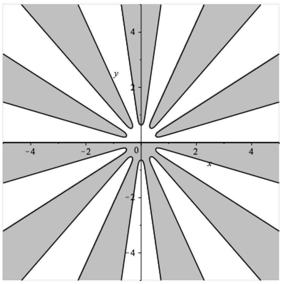 Figure 1
Peer Reviews
No public reviews on file for this paper yet. If you reviewed it on a platform where reviews are public (OpenReview, ICLR, NeurIPS, ICML), you can paste yours below so the community can read it here.
Videos
No videos yet. Explain this paper in a talk, walkthrough, or lecture? Add one.
Fredholm determinant solutions of the Painlevé II hierarchy and gap probabilities of determinantal point processes
Mattia Cafasso
*LAREMA - Université d’Angers, 2 Boulevard Lavoisier, 49045 Angers, France;*[email protected]
Tom Claeys
*Institut de Recherche en Mathématique et Physique, UCLouvain, Chemin du Cyclotron 2, B-1348 Louvain-La-Neuve, Belgium;*[email protected]
Manuela Girotti
*Department of Mathematics, Colorado State University, 1874 campus delivery, Fort Collins, CO 80523 and Department of Mathematics and Statistics, Concordia University, Montréal, QC;*[email protected]
Abstract
We study Fredholm determinants of a class of integral operators, whose kernels can be expressed as double contour integrals of a special type. Such Fredholm determinants appear in various random matrix and statistical physics models. We show that the logarithmic derivatives of the Fredholm determinants are directly related to solutions of the Painlevé II hierarchy. This confirms and generalizes a recent conjecture by Le Doussal, Majumdar, and Schehr [20]. In addition, we obtain asymptotics at for the Painlevé transcendents and large gap asymptotics for the corresponding point processes.
1 Introduction
We consider a family of integral kernels , defined for , of the form
[TABLE]
where , and and are curves in the left and right half of the complex plane without self-intersections which are asymptotic to straight lines with arguments at infinity, as illustrated in Figure 1. The function can be any odd polynomial of the form
[TABLE]
with . Determinantal point processes with kernels of this form appear in various random matrix and statistical physics models. The most prominent example is the Airy kernel, which corresponds to and . A generalized Airy point process characterized by the kernel (1.1) with monomial appeared recently in [20], as a model for the momenta of a large number of fermions trapped in a non–harmonic potential. Point processes with kernels of the general form (1.1), but with not necessarily polynomial, also appear, for instance, in [29]. In [2], a connection was established between the kernels (1.1), the theory of Gelfand–Dickey equations and some specific solutions which are related to topological minimal models of type (see [19] for an excellent introduction to this subject). The monomial case for is also related to spin chains in a magnetic field [35].
Our objective is to derive properties of the Fredholm determinants
[TABLE]
for and , where is the integral operator with kernel acting on . Throughout the paper, in order to distinguish integral kernel operators from their kernels, we will denote integral kernel operators by calligraphic letters ( in the above equation) and the associated kernels by the corresponding uppercase letter ( in the above equation).
Given a determinantal point process on the real line characterized by a correlation kernel , the Fredholm determinant is the probability distribution of the largest particle (which exists almost surely if the Fredholm determinant is well-defined) in the process, , see e.g. [29, 34]. For , is the probability distribution of the largest particle in the associated thinned process, which is obtained from the original process by removing each of the particles independently with probability , see e.g. [8, 10, 11, 12]. In Appendix A, we confirm using standard methods that the kernels (1.1) indeed define a point process for any choice of , and this implies, in particular, that is a distribution function for any .
As our first result, we will prove that can be expressed explicitly in terms of solutions to the Painlevé II hierarchy.
The Painlevé II hierarchy is a sequence of ordinary differential equations obtained from the equations of the mKdV hierarchy via self-similar reduction [23]. Using the same normalization as in [15], the -th member of the Painlevé II hierarchy is an equation for defined as follows:
[TABLE]
where are real parameters, and where the operators are the Lenard operators defined recursively by
[TABLE]
The first members of the hierarchy are111The function corresponds to the function in [20] if we set the parameters to zero.
[TABLE]
where ′ stands for . Generally speaking, even if there exist families of rational and special function solutions to Painlevé equations and hierarchies, one can say that typical solutions are transcendental functions which have no simple closed expression. We construct a family of solutions to the Painlevé II hierarchy in terms of the Fredholm determinants (1.3). This is also of interest from a numerical point of view: whereas it is in general a challenge to accurately evaluate Painlevé transcendents numerically, there are efficient algorithms to compute Fredholm determinants [9].
We will be interested in the homogeneous version of the Painlevé II hierarchy, which corresponds to . The family of solutions that we will construct, contains natural generalizations of the Hastings-McLeod solution [26] and the Ablowitz-Segur solutions [33] to the (second order) Painlevé II equation. These solutions behave like a multiple of the Airy function as . More precisely, for every , we construct solutions of the -th member of the hierarchy in terms of , in such a way that q\big{(}(-1)^{n+1}s;\varrho\big{)} decays rapidly at , and behaves like a root function at if .
Theorem 1.1**.**
Let , , and let be the Fredholm determinant defined in (1.3) with given by (1.1)–(1.2). There is a real solution to the equation of order in the Painlevé II hierarchy (1.4) which has no poles for real , which satisfies
[TABLE]
and which has the asymptotic behavior
[TABLE]
for some . Moreover, if ,
[TABLE]
For any , we also have the identity
[TABLE]
*for in terms of .
In [21], the authors studied for the case of monomial . Generalizing the approach used by Tracy and Widom in [36], they proved that has an explicit expression in terms of a particular solution of the quite simple Hamiltonian system of dimension :
[TABLE]
Namely, . Then, they conjectured that this Hamiltonian system implies that solves the equation of order of the Painlevé II hierarchy, where all the parameters are set to [math]. The conjecture had been verified by the authors up to large , by explicit computations. Theorem 1.1 proves an extended version of this conjecture connecting directly the gap probability of these processes with the Painlevé II hierarchy, without using the Hamiltonian system. It would still be interesting, as suggested by the authors of [21], to find another proof of their conjecture comparing directly (1.11) with the well known Hamiltonian system classically associated to the Painlevé II hierarchy, see [32].
Remark 1.2**.**
More detailed asymptotics for as can in fact be predicted with the following heuristic arguments. If q\big{(}(-1)^{n+1}s;\varrho\big{)} decays rapidly as , it can be expected that the term at the left and the term at the right are dominant in the equation (1.4) for large . The equation then reduces formally to the generalized Airy equation
[TABLE]
and it can therefore be expected that q\big{(}(-1)^{n+1}s\big{)} behaves for large like a real decaying solution of this equation. The function f(s)=\sqrt{\varrho}\,{\mathrm{Ai}}_{2n+1}\big{(}(-1)^{n+1}s\big{)} with
[TABLE]
is such a solution for any , see e.g. [20].
When all the parameters are set to [math], we confirm the above heuristics by proving that, with as in Theorem 1.1,
[TABLE]
(see equation (3.9) below). As explained in Remark 3.1, proving this rigorously for general would require a rather technical saddle point analysis, and we therefore do not pursue this.
Remark 1.3**.**
For , (1.10) is the well-known Tracy-Widom distribution [36], which is among others, for , the limit distribution for extreme eigenvalues in many random matrix ensembles. For general and , (1.10) has the same structure as generalizations of the Tracy-Widom distributions obtained in [15], see also [3], which describe the limit distribution for the extreme eigenvalues in unitary random matrix models with critical edge points. However, we emphasize that the relevant solutions in [15] are different from the ones present here, since they correspond to and have different asymptotics. Therefore, the distribution functions appearing in [15] are different from .
One cannot evaluate the Fredholm determinants explicitly for a given value of , and therefore it is natural to try to approximate them for large values of . In general, the asymptotics can be deduced directly from the asymptotics of the kernel as , but the are more delicate, and are commonly referred to as large gap asymptotics [25, 30]. In our final result, we obtain asymptotics for up to the value of a multiplicative constant. For the sake of clarity, let us first state the result in the simpler case where the parameters are set to [math].
Theorem 1.4**.**
Let and let be the Fredholm determinant defined in (1.3) with given by (1.1) and monomial . As , there exists a constant , possibly depending on , such that we have the asymptotics
[TABLE]
with if and otherwise. Moreover, the asymptotics (1.9) can be improved to
[TABLE]
Remark 1.5**.**
The leading order term of as , namely , was already predicted in [20], but without any information about the subleading terms. Our approach to prove Theorem 1.4 consists of first deriving asymptotics for the logarithmic derivative , which we then integrate in . A consequence is that the multiplicative constant in (1.14) arises as a constant of integration, which we are not able to evaluate. Explicitly evaluating such multiplicative constants in large gap asymptotics of Fredholm determinants is in general a difficult task, see [30]. In the Airy case with , it was proved in [18, 4] that , where is the derivative of the Riemann function, by approximating the Fredholm determinant by a Toeplitz or Hankel determinant for which the corresponding constant can be obtained via the evaluation of a Selberg integral. It seems unlikely that a similar approach could lead to the evaluation of for .
In the more general case where the parameters are different from zero, the asymptotics of change in a rather subtle way; we refer to Section 4 for further details. Let
[TABLE]
and define and as follows:
[TABLE]
where the residue at infinity is minus the coefficient of in the large expansion of the branch of which is positive for large , and similarly
[TABLE]
We will explain in Section 4 that these numbers are related to topological minimal models of type and, more specifically, to flat coordinates for the corresponding Frobenius manifolds. One can also compute as follows:
[TABLE]
We can now state our result on large gap asymptotics in full generality.
Theorem 1.6**.**
Let , , and let be the Fredholm determinant defined in (1.3) with given by (1.1)–(1.2). As , there exists a constant , possibly depending on and the parameters , such that we have the asymptotics
[TABLE]
with if and otherwise. Moreover, the asymptotics (1.9) can be improved to
[TABLE]
For , there are no parameters of deformation , so that Theorem 1.6 gives the well known large gap asymptotics for the Tracy–Widom distribution [4, 18, 36]
[TABLE]
In the first non-trivial case , we obtain
[TABLE]
In the case , we have two deformation parameters , and the large gap asymptotics read
[TABLE]
When increases, formulas get longer and longer, but they remain always completely explicit.
Let us end this introduction with an outline for the rest of this paper. In Section 2, we will show that the Fredholm determinants are equal to Fredholm determinants of a simpler integral operator, obtained through Fourier conjugation. This crucial observation will allow us to show that can be written as the Fredholm determinant of an operator which is of integrable type. We then use the formalism developed by Its, Izergin, Korepin, and Slavnov [28] to express the logarithmic derivative of in terms of a Riemann–Hilbert (RH) problem. We show that this RH problem is equivalent to a special case of the RH problem associated to the Painlevé II hierarchy. This enables us to prove formula (1.10). In Section 3, we will apply the Deift–Zhou steepest descent method to obtain asymptotics for the Painlevé II RH problem and to prove the asymptotics (1.8) for the Painlevé transcendent q\big{(}(-1)^{n+1}s;\varrho\big{)}. In Section 4, we perform a similar but somewhat more complicated asymptotic analysis as , which will lead to the proof of (1.9), and to the proof of the large gap asymptotics stated in Theorems 1.4 and 1.6. An important ingredient in this analysis is the construction of a suitable -function, for which we need to exploit results related to the theory of topological minimal models of type . The general strategy to prove Theorem 1.4 and Theorem 1.6 shows similarities with the one from [13], where large gap asymptotics were obtained for Fredholm determinants arising from product random matrices. Finally, in Appendix A, we prove that the kernels (1.1) define point processes.
2 Painlevé expression for the Fredholm determinant
This section is devoted to the proof of (1.7) and (1.10). In the following we denote with the indicator function of the contour , and analogously for . Let be a kernel of the form (1.1). We will start by showing that the Fredholm determinant is equal to the Fredholm determinant of another integral operator with kernel which is of integrable type, according to the terminology of Its, Izergin, Korepin, and Slavnov [28]. This means that has the form
[TABLE]
for some column vectors which are such that .
Proposition 2.1**.**
Let be the kernel of the form (2.1) with
[TABLE]
and the associated operator acting on . Then we have
[TABLE]
Proof.
Using the fact that , one can write the operator in block form as
[TABLE]
where and are respectively given by the kernels
[TABLE]
This implies that the operators and (and hence ) are Hilbert–Schmidt, since
[TABLE]
and analogously for . We need a bit more and prove that actually and are also trace class, such that the Fredholm determinant of is well defined. To see this, introduce a third contour which does not intersect with and . We start with and we introduce two operators
[TABLE]
with kernels
[TABLE]
With the same computation as in (2.6), we prove that both and are Hilbert-Schimdt operators. Moreover, a residue argument shows that
[TABLE]
hence is a trace-class operator. For the operator , the same reasoning applies if we define the operators
[TABLE]
with kernels
[TABLE]
Hence we can use the following chain of equalities
[TABLE]
where has kernel
[TABLE]
It is now important to observe that the above arguments are valid also if we replace the contour by . It is indeed easy to see that if we replace by in (2.6), the operators and are still Hilbert-Schmidt, therefore is still trace class. Moreover, replacing by does not modify the Fredholm determinant , because in the series definition of the Fredholm determinant the contour can be deformed to , by analyticity of the kernel.
The last step of the proof consists in performing a conjugation of by the Fourier-type transform
[TABLE]
with inverse
[TABLE]
The resulting operator has the following kernel, with ,
[TABLE]
where we passed from the first to the second line by deforming the outer integration contour to the right/left depending the sign of , and by computing the residue in . Combining the equations (2.17) and the one above we obtain
[TABLE]
proving (2.3). ∎
Now, following [28], we associate to the integrable kernel a RH problem with jumps
[TABLE]
on the contour and regular asymptotics at infinity. It was proved in [7, Appendix A] that the logarithmic derivative of , if it exists, can be expressed in terms of the solution of a RH problem. Note that for , we have that is smooth and positive, such that exists for all . Then, we have the identity222In the more general identity stated in [7, Appendix A], an additional (explicit) term is present, but this term vanishes in our situation.
[TABLE]
where is the derivative of with respect to , and is the unique solution to the RH problem below.
RH problem for
- (a)
is analytic,
- (b)
has continuous boundary values as is approached from the left () or right () side, and they are related by
[TABLE]
- (c)
there exists a matrix independent of (but depending on and ) such that satisfies
[TABLE]
The identity (2.23) yields the following result.
Proposition 2.2**.**
The Fredholm determinant satisfies the differential identity
[TABLE]
where is defined by (2.26).
Proof.
Starting from formula (2.23), we compute the integral on the right hand side using residues, as done in [6]. We briefly repeat the procedure (which simplifies in our case) here. We start by noting that the jump matrix can be factorized as
[TABLE]
where is a (piecewise) constant matrix on the contours . Here we are using the Pauli notations
[TABLE]
Hence, we obtain
[TABLE]
where, in the last line, we used the cyclic property of the trace and the form of . Now, we observe that the integral contributions of the minus sides of and sum up to zero, and that the plus sides can be deformed to a large counterclockwise circle of radius , leading to
[TABLE]
In the last equality we used the fact that has zero trace, since has determinant equal to .
The relation with the second Painlevé hierarchy is established by transforming the RH problem for to one with constant jumps. Namely, define
[TABLE]
Then it is straightforward to verify that solves the following RH problem:
RH problem for
- (a)
is analytic, with as in Figure 2,
- (b)
the boundary values of on are related by the conditions
[TABLE]
- (c)
has the following behavior at infinity:
[TABLE]
where
[TABLE]
and
[TABLE]
Note that we have now chosen to orient both jump contours from left to right, so that , but with reverse orientation, and . Note also that the RH solution depends on the choice of jump contours , but that the solution corresponding to a different choice of jump contours can be obtained by analytic continuation. The matrix is independent of the choice of jump contours.
The above RH problem is equivalent to the one in [15, Section 4.2], in the case where and where the Stokes multipliers are given by
[TABLE]
Proposition 2.3**.**
Let and let be the solution to the above RH problem. Then, the function
[TABLE]
is real for , , and it solves the Painlevé II hierarchy equation (1.4).
Proof.
We start by showing that satisfies two symmetry relations, provided that we choose and in such a way that333To be more precise, as oriented contours, while as sets, but they have opposite orientation. . First, we verify that satisfies the RH problem for . But since the RH solution is unique (this follows from standard arguments using Liouville’s theorem), we obtain the identity
[TABLE]
Similarly we obtain, for real values of , the relation
[TABLE]
These identities imply in particular that
[TABLE]
It follows that the two expressions at the right hand side of (2.35) are indeed equal, and moreover that is real-valued.
The remaining part of the proof consists of identifying with solutions to the Lax pair associated with the Painlevé II hierarchy (cf. [16, 23, 31, 32]). Here we use the same approach and normalization as in [15, Section 4.1]. Namely, if we define
[TABLE]
then one verifies using the RH conditions that satisfies the differential equation
[TABLE]
with as in (2.35). In addition, we have a second differential equation of the form
[TABLE]
with as in [15, Equations (4.1)–(4.3)]. The compatibility between the Lax equations (2.36) and (2.37) now implies, in the same way as in [15], that solves the Painlevé II hierarchy equation (1.4).
Remark 2.4**.**
In particular, the solution is uniquely determined by the Stokes parameters described in the Riemann–Hilbert for .
We are now ready to prove (1.7).
Proposition 2.5**.**
Let be defined by (1.3), and by (2.35). Then, we have the differential identity
[TABLE]
Proof.
It follows from (2.36) that is a polynomial in . Hence, the term in in the large expansion of vanishes, and this yields
[TABLE]
where and are defined by the expansion
[TABLE]
In particular, the -entry of (2.39) gives
[TABLE]
Using (2.40) together with Proposition 2.2 and the relation (see (2.33)), we obtain the result.
Since is real-valued, the above proposition implies that is concave as a function of . We also know that is a distribution function for , so we can conclude that
[TABLE]
Hence, integrating (2.38), we obtain
[TABLE]
and after another integration by parts we obtain (1.10).
3 Asymptotics for the Painlevé function as
We start from the RH problem for , see (2.30)–(2.32), and we rescale it in the following way. Let
[TABLE]
then satisfies the following RH problem.
RH problem for
- (a)
is analytic in , where and are the transformed contours under the scaling ,
- (b)
satisfies the jump relations
[TABLE]
- (c)
as , we have
[TABLE]
where
[TABLE]
We now note that, by (2.34),
[TABLE]
as , uniformly for and for in any compact set. For this reason we want to choose the contours and in such a way that
[TABLE]
Even in the case where the parameters are not all equal to zero, the behavior of the phase is still asymptotically dominated by the leading terms as . It is straightforward to check that we can always choose and such that the inequalities above are satisfied. This is also illustrated in Figure 3.
With such a choice of and , the jump relation for reads as ,
[TABLE]
for a suitable constant , uniformly in . By small norm theory for RH problems (see e.g. [17, 27]), we can infer that there exists a constant such that
[TABLE]
uniformly in . This implies in particular, by (2.35) and (3.4), that
[TABLE]
as , which proves (1.8).
If we want more precise asymptotics, we need to use the integral equation
[TABLE]
which is satisfied by as a consequence of the RH conditions, with and . To see this, one verifies that the right hand side of the above equation satisfies the three RH conditions for . Uniqueness of the RH solution then yields the integral equation (see, for instance, [24]). This integral equation implies that
[TABLE]
Using also (3.8), we obtain
[TABLE]
as . It follows from (2.35) that
[TABLE]
as . If , it follows directly from the substitution and (1.12) that
[TABLE]
as already announced in the introduction.
Remark 3.1**.**
In order to prove (3.9) for general , we would need the asymptotics of the integral . These can in principle be obtained using saddle point arguments, but this would require a lot of technical work, especially because the integrand depends on the large parameter in a rather complicated manner. We therefore do not aim to prove this.
4 Asymptotics for as
In this section, we restrict to the case where , and we analyze the RH problem for in the limit , in order to derive asymptotics for as and large gap asymptotics for .
4.1 Construction of the -function
In the asymptotic analysis as , we were able to normalize the RH problem for simply by multiplying at the right by the factor . However, for negative, the topology of the set is different from the one sketched in Figure 3, and forces us to normalize the RH problem for in a different way, namely by means of the construction of a suitable -function.
We define a function of the form
[TABLE]
with analytic in and such that it behaves like as .
We fix the constants and the branch point by the requirement that there exists a value such that
[TABLE]
It was shown in [15, Section 4.6.2] that this yields the following asymptotic formulas as ,
[TABLE]
and
[TABLE]
The aim of the rest of this subsection is to give more explicit asymptotics for and , which will be needed later on.
Lemma 4.1**.**
Suppose that is sufficiently large, set , and let be the unique positive solution to the equation
[TABLE]
If we define
[TABLE]
for , then defined by (4.1) has the asymptotics (4.2).
Proof.
If we expand defined by (4.1) and defined by (2.34) as , we obtain in a straightforward manner that (4.2) implies
[TABLE]
as . Equating the coefficients of of the left and right hand side, we obtain the system of equations
[TABLE]
The equations in (4.8) form a linear system with unknowns and as a parameter in triangular form, whose solution is given by (4.7). Substituting this into (4.9), we obtain
[TABLE]
Moreover,
[TABLE]
and
[TABLE]
by the binomial formula. Substituting the latter two identities into (4.1), we obtain (4.6). For sufficiently large , we observe easily that (4.6) has a unique positive solution, since it reduces to
[TABLE]
in the large limit.
For , as a first step, we need the following identity.
Lemma 4.2**.**
Set . The constant defined by (4.2) is given by
[TABLE]
Proof.
The proof is analogous to that of Lemma 4.1. Namely we expand as , but now we take into account one more term:
[TABLE]
as , and this leads to
[TABLE]
Plugging the values (4.7) of into the equation above and performing some straightforward computations as in (4.1) we finally obtain (4.11).
We will now derive a large expansion of . First we need the following lemma:
Lemma 4.3**.**
Let be a positive integer and . Define the polynomial as
[TABLE]
For large positive , there is a unique positive solution of the equation . It admits a Puiseux series at of the form
[TABLE]
with
[TABLE]
where the residue at infinity is equal to minus the term in of the expansion of as , and where we take the branch of which is positive for large .
Proof.
It is a standard fact that there is a unique positive solution to the polynomial equation for sufficiently large, and that it has an expansion of the form (4.12). All the coefficients can be computed recursively by plugging (4.12) in the equation
[TABLE]
and by solving term by term. In this way, we immediately find the value of . For the other terms, it is convenient to rewrite the residue using as coordinate. Indeed, since because of (4.12) we have
[TABLE]
then
[TABLE]
which proves the stated result.
Remark 4.4**.**
*For the interested reader, we mention a connection between the above result and flat coordinates for a special class of Frobenius manifolds, the ones related to topological minimal models of type .
Consider a polynomial as in Lemma 4.3. By shifting the variable , we can assume without any loss of generality that . Define the complex manifold *
[TABLE]
At each point we identify the tangent space with the algebra
[TABLE]
Moreover, we equip this algebra with the bilinear pairing defined by
[TABLE]
The multiplication on and the bilinear pairing satisfy a certain compatibility condition which, together with some additional structures that are not important here, turns into a Frobenius manifold; the one associated to the singularity of type (see for instance [19, 22] and references therein). The coefficients in Lemma 4.3 (up to a rescaling and a permutation necessary to identify the first coordinate with the unit vector field) are the flat coordinates associated to the given Frobenius structure (see, for instance, Corollary 4.6 in [22]). With a different approach, flat coordinates of Frobenius manifolds are also used in [2], in relation with the same type of generalized Airy kernels.
Proposition 4.5**.**
Let
[TABLE]
and
[TABLE]
Then, the positive solution of (4.6) has the asymptotic expansion
[TABLE]
Moreover,
[TABLE]
or equivalently
[TABLE]
In particular,
[TABLE]
Proof.
We apply Lemma 4.3 to the polynomial
[TABLE]
which satisfies . The lemma then implies that
[TABLE]
as , or equivalently
[TABLE]
The result (4.13) now follows by observing that
[TABLE]
and that
[TABLE]
This directly implies (4.15). To see (4.16), we apply Lemma 4.3 to the polynomial . From (4.16) and the definition of , we deduce (4.17).
Given the expansion of , we can now also deduce the one for , as stated in the next proposition.
Proposition 4.6**.**
There exists a constant such that
[TABLE]
Proof.
Using (4.11) and the asymptotic expansion of for , we observe that has an expansion of the form
[TABLE]
Let us now recall the definition of as in Proposition 4.5, such that with and . We also write
[TABLE]
such that by Lemma 4.2. Using the identity , we obtain the relation
[TABLE]
and this results in
[TABLE]
Combining this identity with (4.19) and (4.15) and integrating in , we obtain the result, with unknown integration constant .
4.2 Normalization of the RH problem
We now take the jump contours and of a special form. It is convenient for us to take them such that and coincide with the real line on the interval , and such that they are independent of . Then we define
[TABLE]
now satisfies the following RH problem.
RH problem for
- (a)
is analytic in , with
[TABLE]
as in Figure 4.
- (b)
has the jump relations
[TABLE]
which follows from the fact that for .
- (c)
as , with
[TABLE]
It is easy to see, by studying the argument of the terms in (4.1), that the -function satisfies the following relations:
[TABLE]
for sufficiently large , if we choose the angles between and the real line sufficiently small. Furthermore,
Lemma 4.7**.**
[TABLE]
for sufficiently large .
Proof.
Following the arguments of [15, Section 4.6], we consider the subinterval . For , the analysis is similar.
We set
[TABLE]
From the asymptotic behavior of the coefficients and the endpoint (see (4.3)–(4.5)), we have that
[TABLE]
for (i.e. ). In order to prove that on , we need to prove that the sum appearing in the above expression is negative.
Using Jacobi polynomials and their representation as hypergeometric functions (in particular formula (22.5.42) from [1]), we have that
[TABLE]
On the other hand, using an alternative hypergeometric representation for Jacobi polynomials (formula (22.5.45) from [1]), we have
[TABLE]
for , and this implies the result. ∎
4.3 Construction of the global parametrix
From (4.25), (4.26), and (4.27), it follows that the jump matrices for are exponentially close to the identity matrix as , as long as we stay away from the interval . For this reason, we can expect that, away from , a first approximation to will be given by a function which has the same jump on and the same asymptotic behavior as . This motivates the RH conditions for the global parametrix given below.
RH problem for
- (a)
is analytic in ,
- (b)
has the jump relation
[TABLE]
- (c)
as .
If we impose in addition that as , then it is a well-known fact, see e.g. [17], that the solution is given by
[TABLE]
where is analytic on and as .
Indeed, the jump relation for can be easily verified by noticing that for . The asymptotic behavior at infinity follows by expanding the function : more precisely, we have
[TABLE]
4.4 Construction of local Airy parametrices
As blows up as , we cannot expect it to be a good approximation to close to . Let us therefore take sufficiently small disks around , and construct local parametrices in these disks, which have the same jump relations as on the parts of the jump contour inside , and which match with the global parametrix on . To build the parametrices, we use a standard construction using the Airy function, see e.g. [17, 27] as general reference, and [14] for a construction which is almost identical to the present one.
Define the functions in terms of the Airy function,
[TABLE]
with , and define the functions
[TABLE]
The functions , , are entire functions, and by the Airy function identity , they satisfy the relations
[TABLE]
Moreover, if we define sectors , , and , then we have
[TABLE]
as in the sector , where we take the plus sign in the lower half plane and the minus sign in the upper half plane.
Let us now focus on the disk . We define a conformal map by the equation
[TABLE]
where the minus sign is taken in the upper half plane and the plus sign in the lower half plane. Then it is straightforward to verify that maps to a neighbourhood of .
We now define the local parametrix as
[TABLE]
where we take as follows: if is in the sector between and , for in the sector between and , and for in the sector between and . If is analytic in , then satisfies the same jump relations as inside , and we additionally fix the matrix by the requirement that
[TABLE]
uniformly for , as . Therefore, we take
[TABLE]
We can make the matching condition more precise and have, using (4.33) and (4.38),
[TABLE]
uniformly for , as .
The parametrix near can be constructed similarly. Namely, we set for . We then have
[TABLE]
uniformly for , as .
4.5 Small norm RH problem
Finally, we define as
[TABLE]
where stands for both local parametrices at the endpoints .
The function solves the RH problem:
RH problem for
- (a)
is analytic in , where is depicted in Figure 5,
- (b)
has the jump relations
[TABLE]
where takes the form
[TABLE]
for some , uniformly in as , with
[TABLE]
by (4.43) and (4.44), and for some matrix independent of ,
- (c)
as .
Using the general theory of RH problems normalized at infinity and with jump matrices close to the identity, see e.g. [17, 27], we can conclude that as , is close to the identity and has asymptotics of the form
[TABLE]
for some matrices and which are independent of and which can be computed via a recursive procedure. We explain how this works for the matrix . Because of the RH conditions for , we know that as , and expanding the jump relation for in , we obtain
[TABLE]
whereas is analytic everywhere else in the complex plane. This allows us to deduce that is given by
[TABLE]
This can be computed explicitly using residue calculus. As , there are matrices , independent of such that we have
[TABLE]
The entries of and can be computed explicitly by carefully expanding as . We have in particular that
[TABLE]
by (4.7) after a straightforward calculation. It follows that, for outside ,
[TABLE]
Expanding this as , we get
[TABLE]
and this implies finally that
[TABLE]
as , where the matrix can be computed in terms of the jump matrix . The components of are however unimportant for our concerns.
4.6 Asymptotics for q\big{(}(-1)^{n+1}s;1\big{)} and for as .
We are now ready to compute the asymptotics for as , as stated in (1.9) and (1.20). Using first (2.35) and (4.24), and then the fact that for large together with (4.34) and the large asymptotics for , we obtain
[TABLE]
By (4.14), (4.50) and (4.51), we get
[TABLE]
as , where and are as in (4.13). This proves (1.9) and the improved version (1.20), up to the value of .
To obtain large gap asymptotics, we follow two different routes, and the compatibility between them will allow us to evaluate . First, we use (4.53) to compute
[TABLE]
as , where
[TABLE]
In addition, by Lemma 4.5. Substituting this into (1.10) and integrating, we obtain
[TABLE]
as , for some constant .
Secondly, we start from (2.27), which by (2.33) and (4.24) implies
[TABLE]
[TABLE]
as . By (4.18) and (4.50), we obtain after integration that there is a constant such that
[TABLE]
This completes the proof of Theorem 1.6 and Theorem 1.4. Comparing this with (4.55), we find
[TABLE]
Substituting this in (4.53), we complete the proof of (1.20).
Acknowledgements.
M.C. and M.G. acknowledge the support of the H2020-MSCA-RISE-2017 PROJECT No. 778010 IPaDEGAN. T.C. was supported by the Fonds de la Recherche Scientifique-FNRS under EOS project O013018F. Part of the work of M.C. and M.G. was done during their visits at the Institut de Recherche en Mathématique et Physique (UCLouvain) in May 2018. We acknowledge UCLouvain for excellent working conditions and generous support. Part of the work was as well conducted during M.C. and M.G.’s visit at Concordia University in July 2018. We thank Concordia University for hosting us and providing numerous resources and facilities for performing our work. M.C. wants to thank Marco Bertola for many interesting discussions on point processes and integrable operators and, in particular, for teaching him the techniques used in the appendix below to prove that the kernels analyzed in this paper define determinantal point processes.
Appendix A The generalized Airy kernel point processes
The generalized Airy kernel studied in [20] is given by
[TABLE]
where
[TABLE]
is a real solution of the equation
[TABLE]
Proposition A.1**.**
The kernel (A.1) is equal to (1.1) with .
Proof.
By (1.12), we have
[TABLE]
since for and .
In [20] the authors obtained as the scaling limit of the kernels associated to certain point processes describing the momenta of non–interacting fermions trapped in a non–harmonic potential. In what follows we will prove, without references to any physical model, that indeed, for any as in (1.1) and as in (1.2) , the determinants
[TABLE]
are the correlation functions associated to a well defined point process. The proof uses Theorem 3 in [34], stating that a Hermitian locally trace class operator uniquely defines a determinantal point process if and only if it is positive definite and bounded from above by the identity operator.
Theorem A.2**.**
For any , there exists a unique determinantal point process whose correlation functions are given by (A.5).
Proof.
For future use, we start by rewriting the kernel as
[TABLE]
where
[TABLE]
From (A.6) we immediately deduce that the integral operator with kernel is Hermitian (since is real) and locally of trace class (because of continuity). In order to prove total positivity, we use the Andréief identity
[TABLE]
giving, in our case,
[TABLE]
Now, in order to prove that is bounded from above by the identity, we introduce the associated (generalized) Airy transform as
[TABLE]
where is the standard Fourier transform such that
[TABLE]
and is the multiplication operator by the function {\rm e}^{i\Big{(}\frac{\lambda^{2n+1}}{2n+1}+\sum_{j=1}^{n-1}\frac{(-1)^{n+j}\tau_{j}}{2j+1}\lambda^{2j+1}\Big{)}}. This is a straightforward generalization of what was done in [5] for the Airy case . Note that, in particular,
[TABLE]
Using the equation above in combination with the definition (A.6) of we obtain
[TABLE]
where is the multiplication operator for the characteristic function . We will use the equation above to prove that is a projection operator, i.e. , which implies that . Indeed, denote with the inversion operator such that
[TABLE]
Since
[TABLE]
we immediately see that
[TABLE]
from which the reproducing property follows immediately.
The reference list from the paper itself. Each links out to its DOI / PubMed record.
- 1[1] M. Abramowitz and I. Stegun. Handbook of Mathematical Functions , volume 55 of Applied Mathematics Series . National Bureau of Standards, 10th edition, 1972.
- 2[2] M. Adler, M. Cafasso, and P. van Moerbeke. Nonlinear PD Es for gap probabilities in random matrices and KP theory. Phys. D , 241(23-24):2265–2284, 2012.
- 3[3] G. Akemann and M. Atkin. Higher order analogues of Tracy–Widom distributions via the Lax method. J. Phys. A , 46(1), 2012.
- 4[4] J. Baik, R. Buckingham, and J. Di Franco. Asymptotics of Tracy–Widom distributions and the total integral of a Painlevé II function. Comm. Math. Phys. , 280(2):463–497, 2008.
- 5[5] E.L. Basor and H. Widom. Determinants of Airy operators and applications to random matrices. J. Statist. Phys. , 96(1–2):1–20, 1999.
- 6[6] M. Bertola. The dependence on the monodromy data of the isomonodromic tau function. Comm. Math. Phys. , 294(2):539–579, 2010.
- 7[7] M. Bertola and M. Cafasso. The Riemann–Hilbert approach to the transition between the gap probabilities from the Pearcey to the Airy process. Int. Math. Res. Not. , 2012(7):1519–1568, 2012.
- 8[8] O. Bohigas and M.P. Pato. Randomly incomplete spectra and intermediate statistics. Phys. Rev. E (3) , 74(3):036212, 6, 2006.