Numerical methods for entrainment and detrainment in the multi-fluid Euler equations for convection
William A McIntyre, Hilary Weller, Christopher E Holloway

TL;DR
This paper investigates numerical methods for modeling convection in climate models using multi-fluid Euler equations, focusing on entrainment and detrainment schemes that improve stability and conservation properties.
Contribution
It derives and analyzes mass transfer schemes between fluids in multi-fluid Euler models, demonstrating stable, conservative, and bounded numerical solutions for convection.
Findings
Identified schemes that are conservative, stable, and bounded for large timesteps.
Demonstrated numerical properties on a well-resolved convection test case.
Maintained properties on staggered grids.
Abstract
Convection schemes are a large source of error in global weather and climate models, and modern resolutions are often too fine to parameterise convection but are still too coarse to fully resolve it. Recently, numerical solutions of multi-fluid equations have been proposed for a more flexible and consistent treatment of sub-grid scale convection, including net mass transport by convection and non-equilibrium dynamics. The technique involves splitting the atmosphere into multiple fluids. For example, the atmosphere could be divided into buoyant updrafts and stable regions. The fluids interact through a common pressure, drag and mass transfers (entrainment and detrainment). Little is known about the numerical properties of mass transfer terms between the fluids. We derive mass transfer terms which relabel the fluids and derive numerical properties of the transfer schemes, including…
Click any figure to enlarge with its caption.
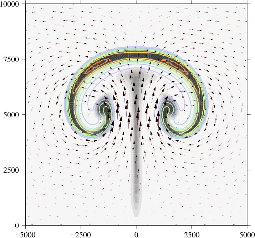 Figure 1
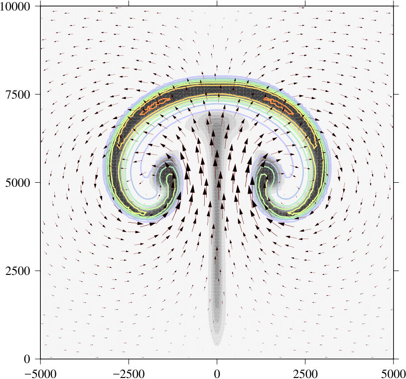 Figure 2
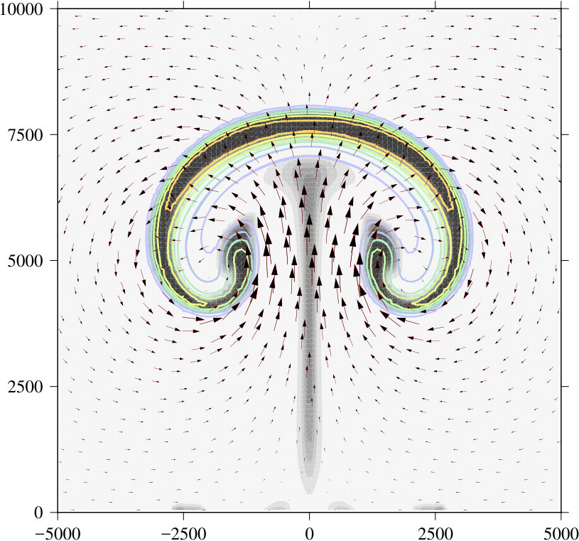 Figure 3
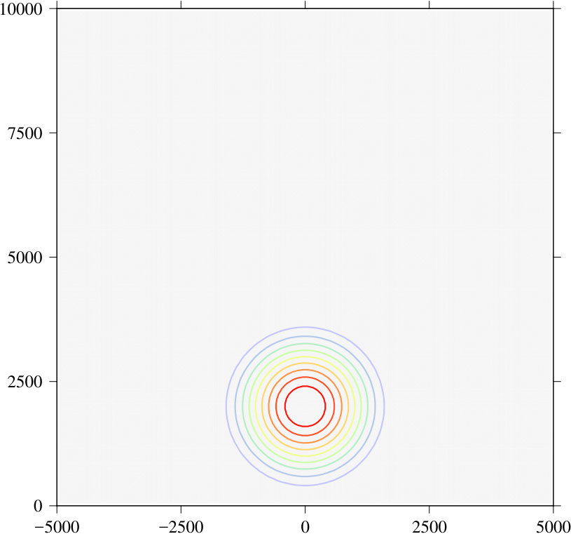 Figure 4
 Figure 5
 Figure 6
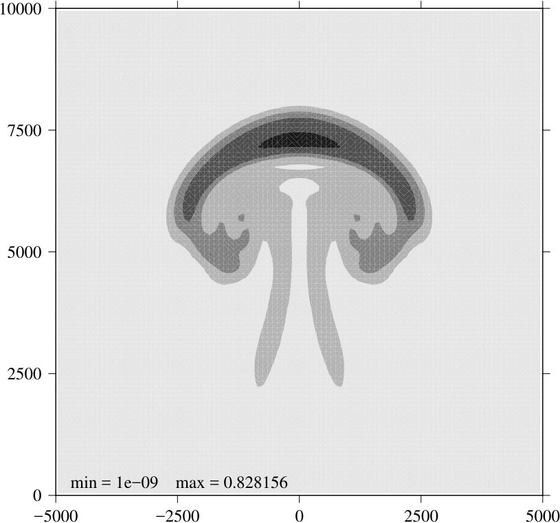 Figure 7
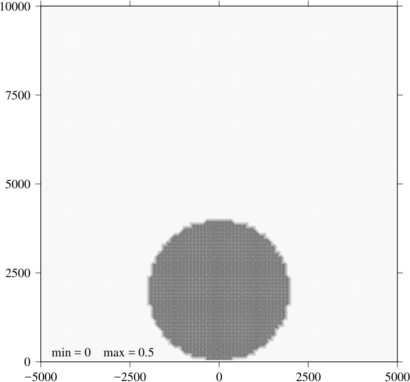 Figure 8
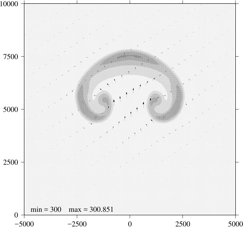 Figure 9
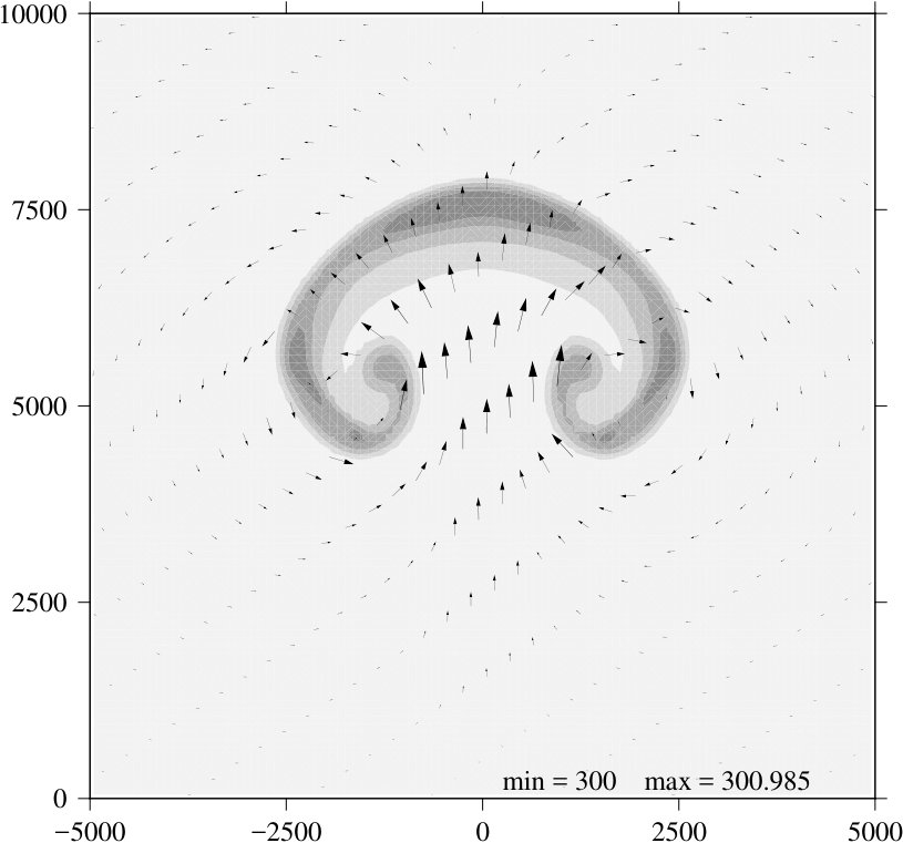 Figure 10
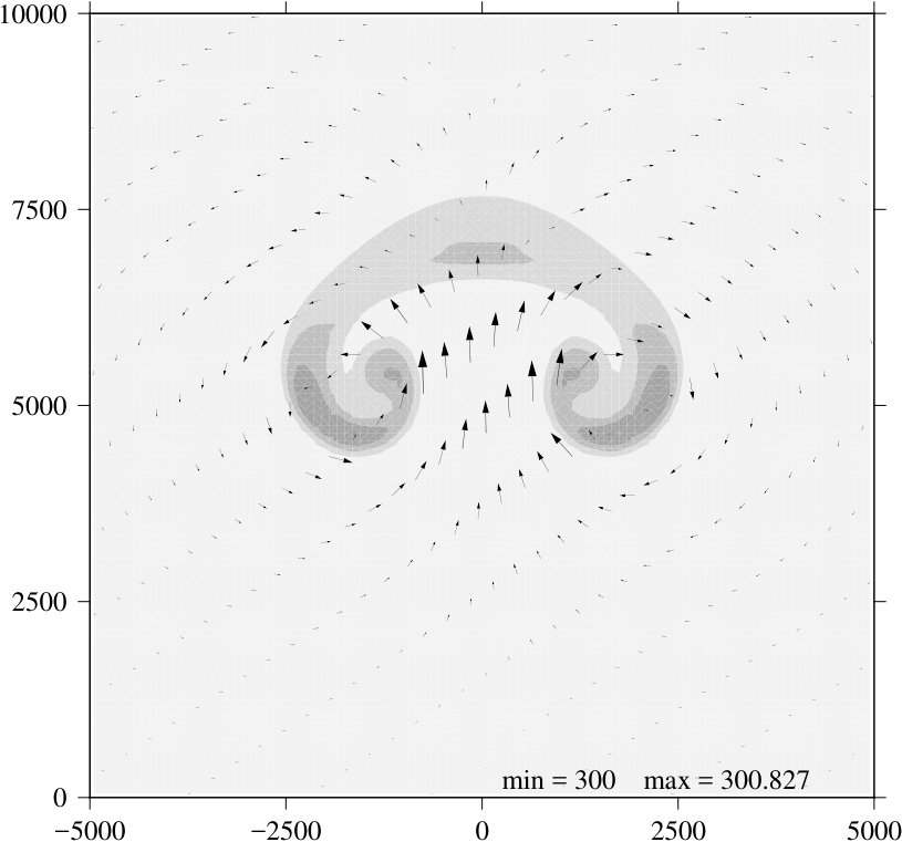 Figure 11
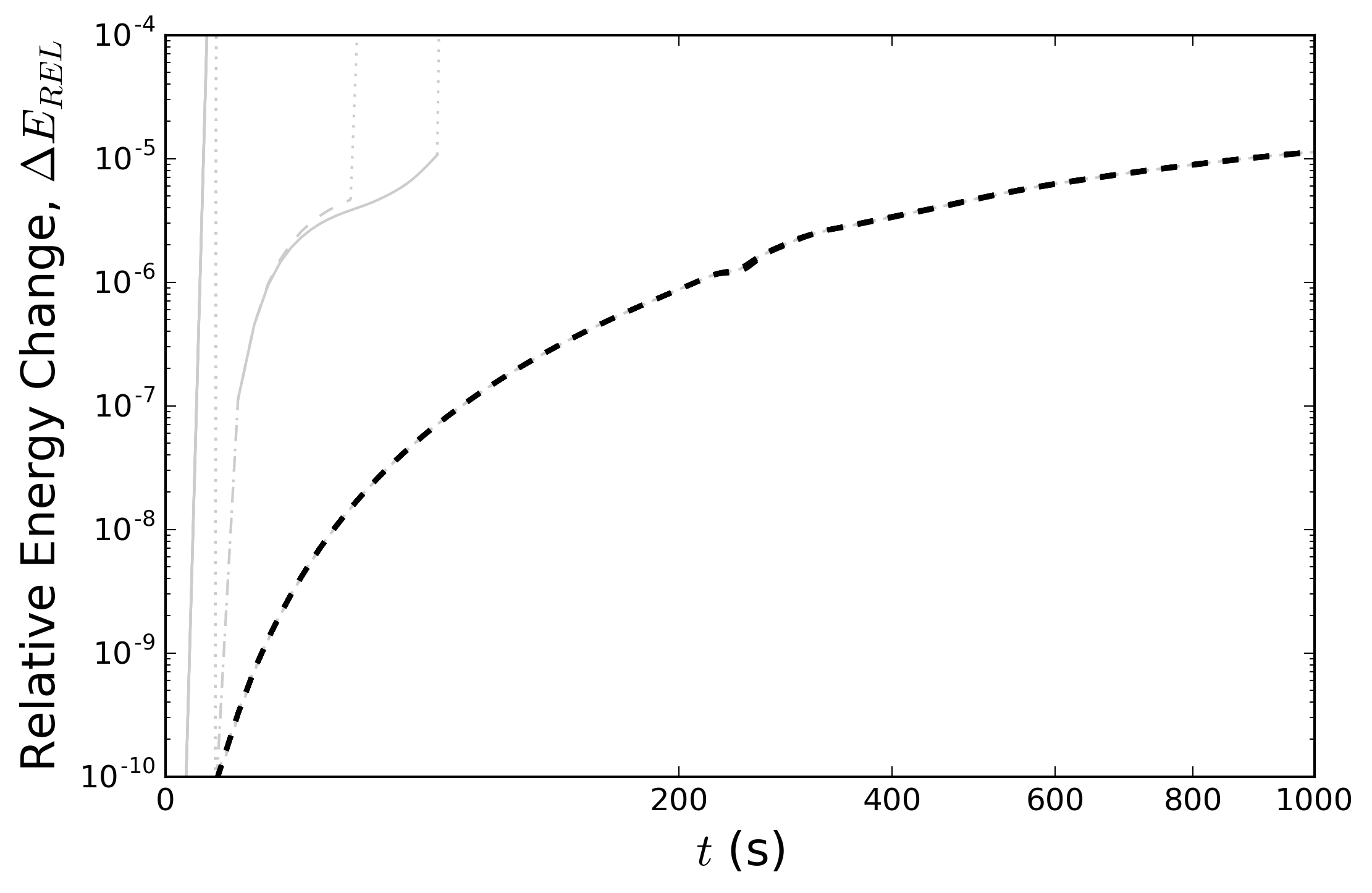 Figure 12
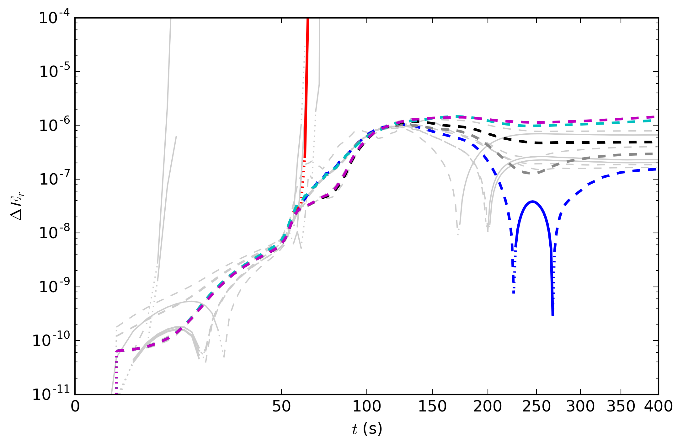 Figure 13
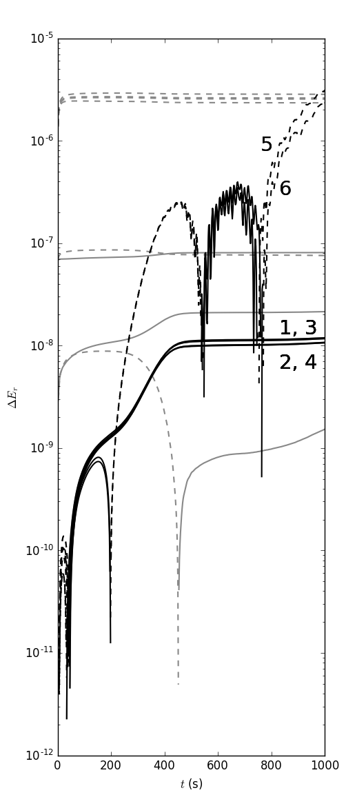 Figure 14
 Figure 15
 Figure 16
 Figure 17
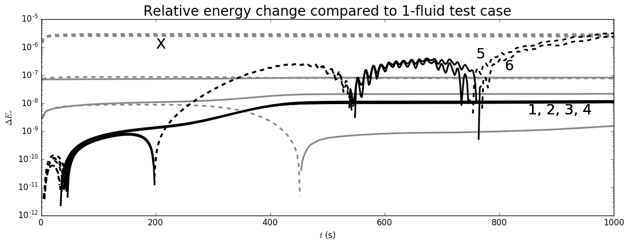 Figure 18
 Figure 19
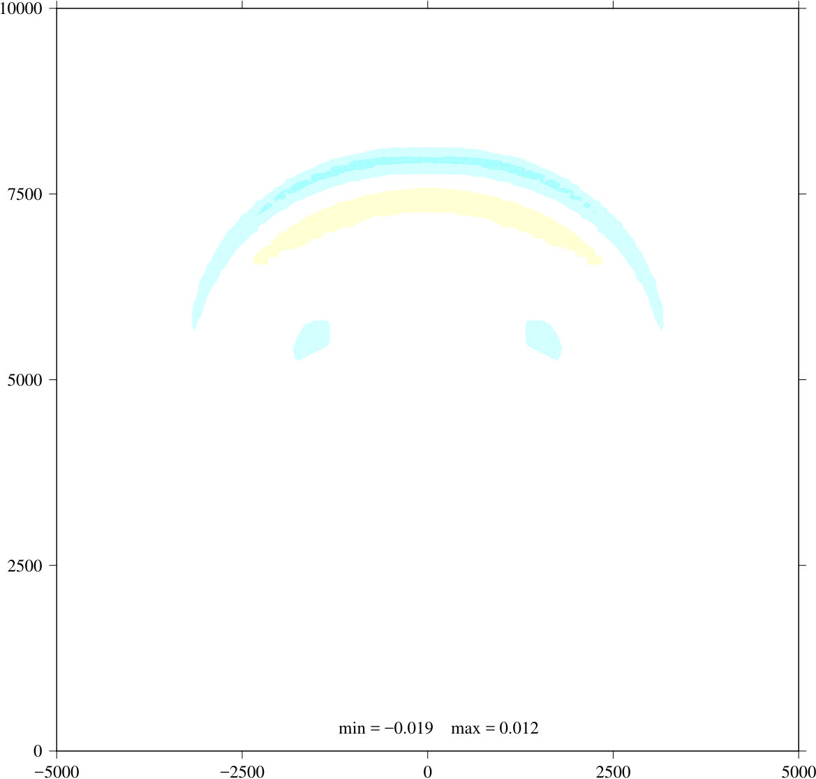 Figure 20
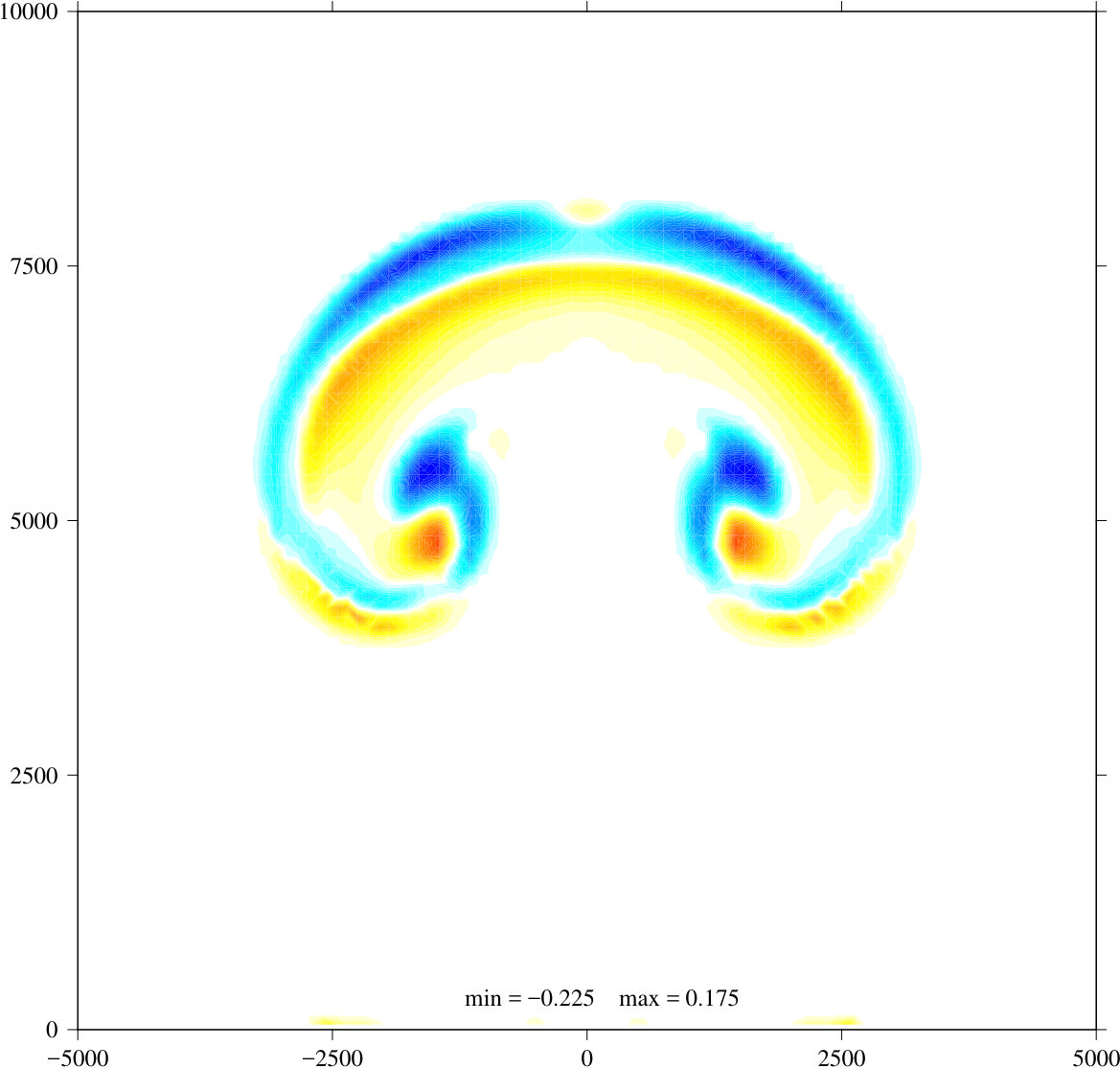 Figure 21
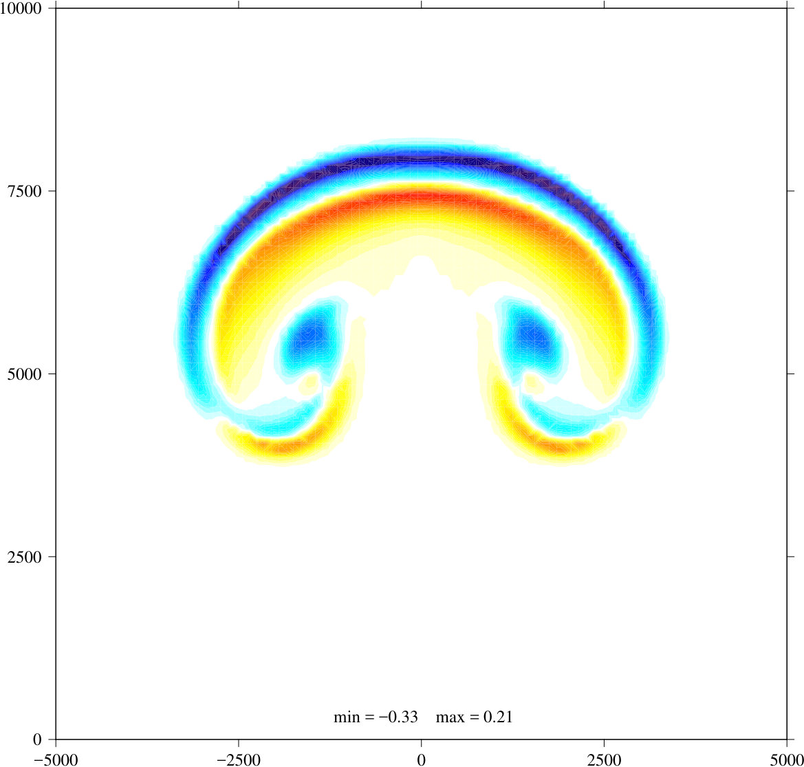 Figure 22
 Figure 23
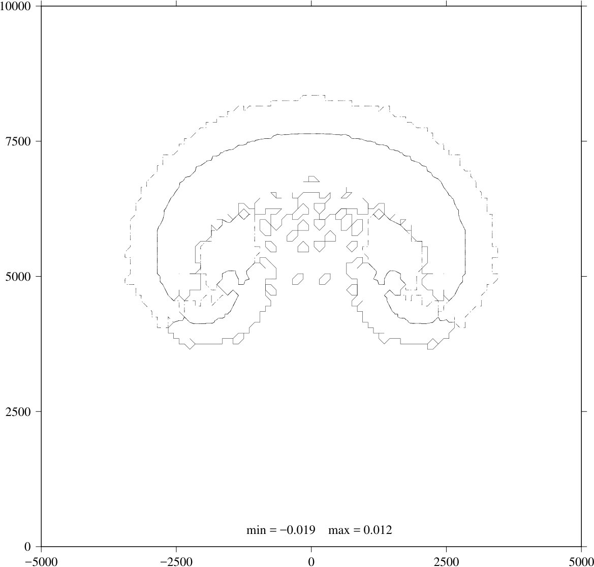 Figure 24
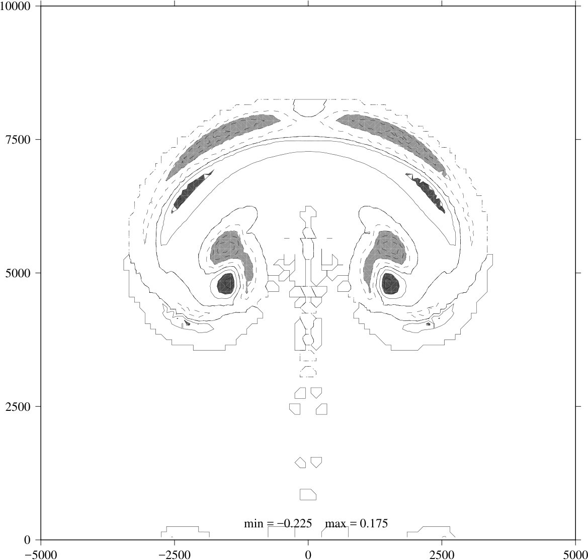 Figure 25
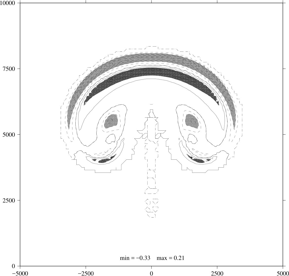 Figure 26
 Figure 27
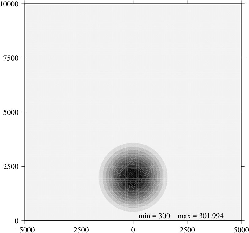 Figure 28
 Figure 29
 Figure 30
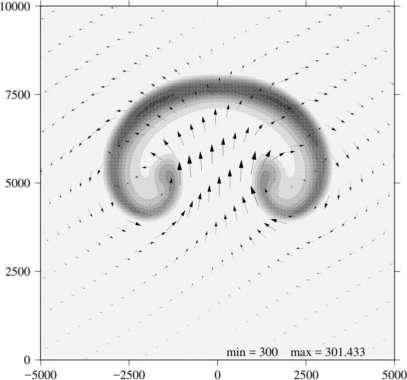 Figure 31
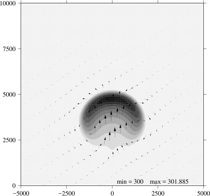 Figure 32
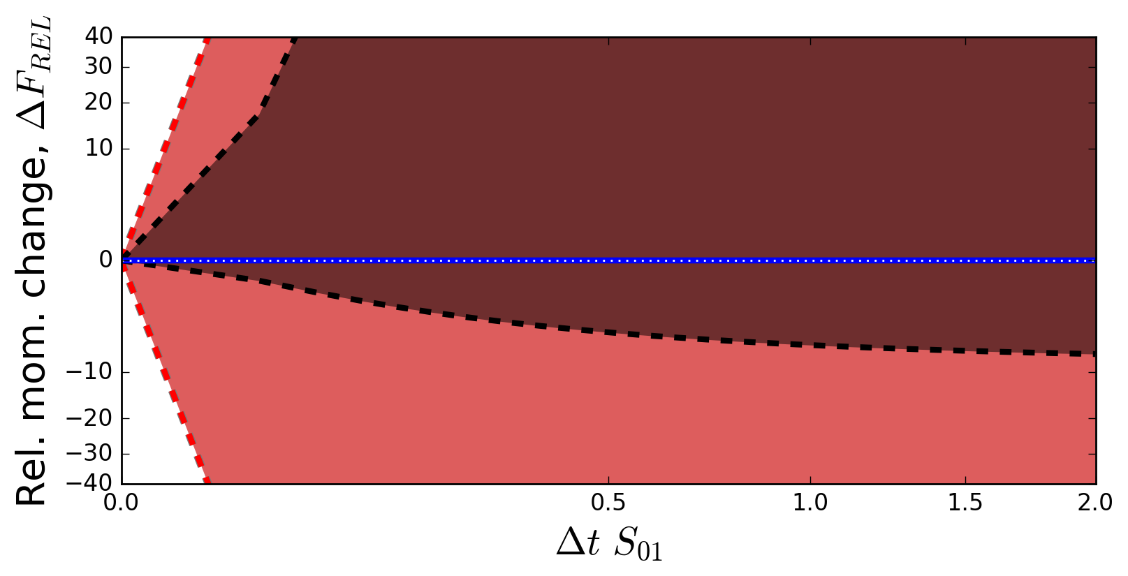 Figure 33
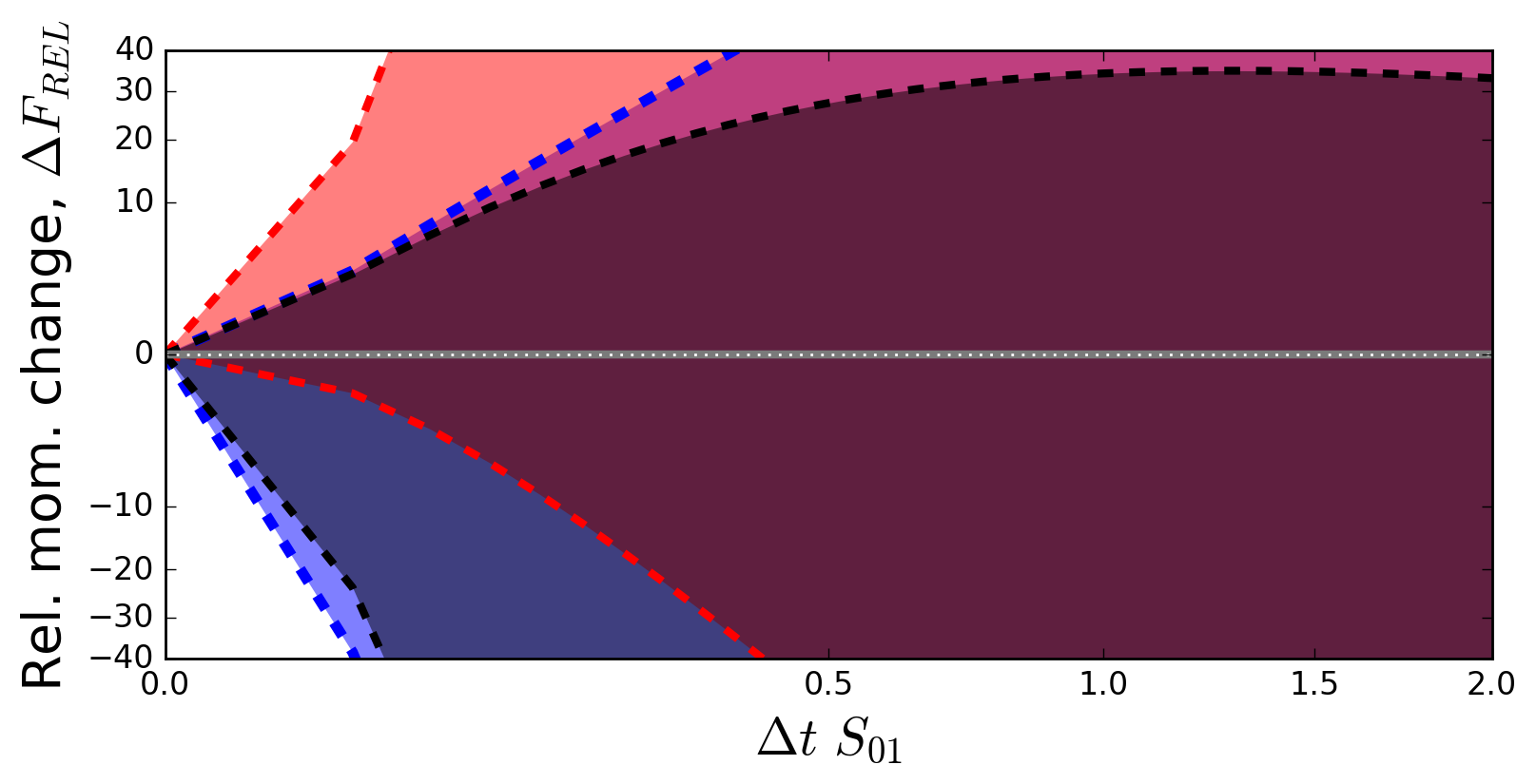 Figure 34
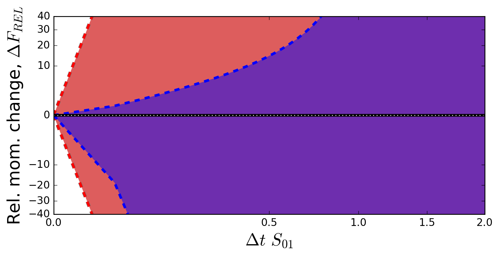 Figure 35
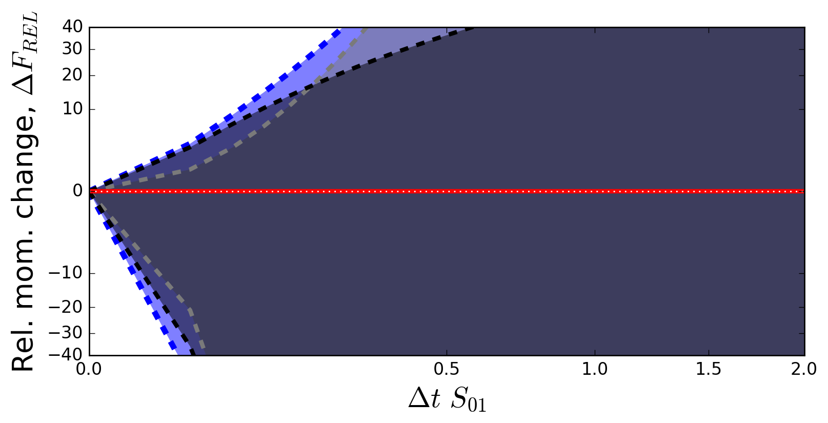 Figure 36
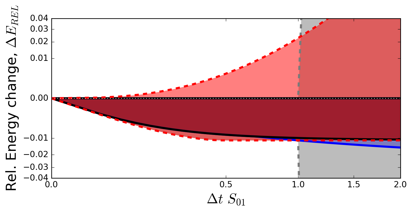 Figure 37
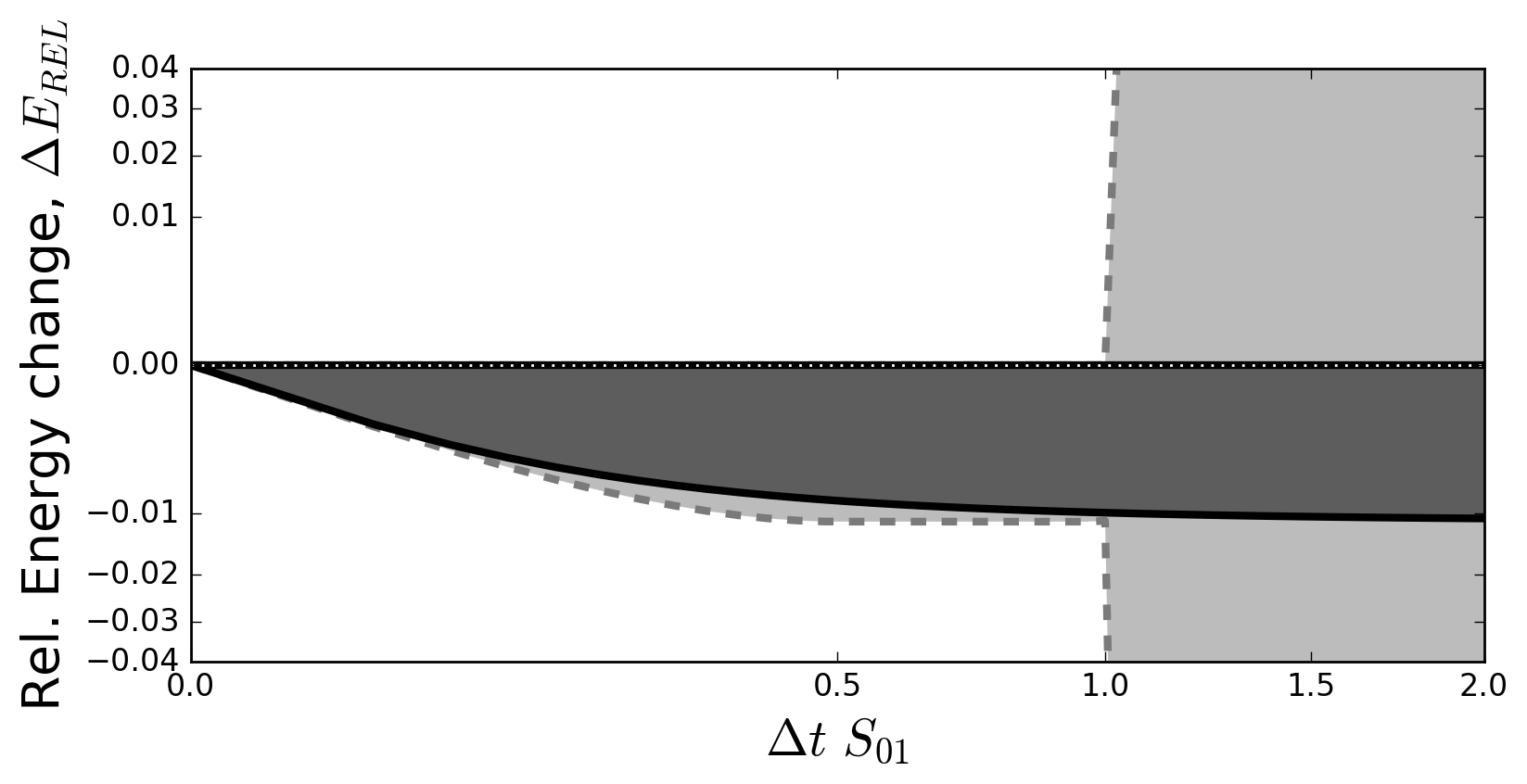 Figure 38
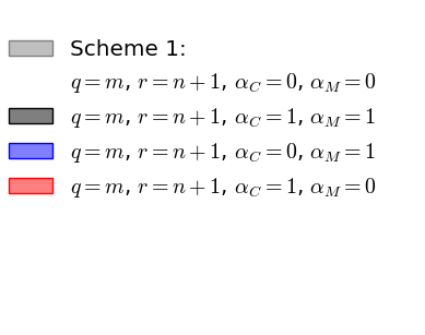 Figure 39
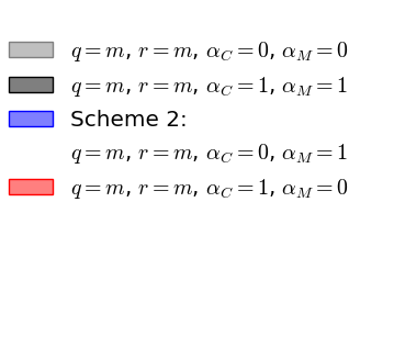 Figure 40
| Scheme | Positive ? | Bounded & ? | \LongunderstackMomentum & | ||
|---|---|---|---|---|---|
| IE conserved? | KE decreases? | ||||
| Method 1 | |||||
| 1 | , , , | ✓ | ✗ | ✓✓ | ✓ |
| 2 | , , , | ✓ | ✓✓ | ✓✓ | ✓✓ |
| 3 | , , , | ✓✓ | ✗ | ✓✓ | ✗ |
| 4 | , , , | ✓✓ | ✓✓ | ✓✓ | ✓✓ |
| Other schemes | ✓ | ✓ for | ✗ | ✗ | |
| Method 2 (Mass-weighted transfers) | |||||
| 5 | , | ✓ | ✓ | ✓✓ | ✓ |
| 6 | , | ✓✓ | ✓✓ | ✓✓ | ✓✓ |
| Other schemes | ✓ | ✓ for | ✓✓ | ✓ for |
| Name | Method | ||||||
|---|---|---|---|---|---|---|---|
| Scheme 1 | 1 | ||||||
| 1 | |||||||
| 1 | |||||||
| 1 | |||||||
| 1 | |||||||
| Scheme 2 | 1 | ||||||
| 1 | |||||||
| 1 | |||||||
| 1 | |||||||
| 1 | |||||||
| Scheme 3 | 1 | ||||||
| 1 | |||||||
| 1 | |||||||
| 1 | |||||||
| 1 | |||||||
| Scheme 4 | 1 | ||||||
| Scheme 5 | 2 | ||||||
| 2 | |||||||
| 2 | |||||||
| Scheme 6 | 2 |
Peer Reviews
No public reviews on file for this paper yet. If you reviewed it on a platform where reviews are public (OpenReview, ICLR, NeurIPS, ICML), you can paste yours below so the community can read it here.
Videos
No videos yet. Explain this paper in a talk, walkthrough, or lecture? Add one.
\papertype
Submitted to QJRMS, 2019 \paperfield
\abbrevsABC, a black cat; DEF, doesn’t ever fret; GHI, goes home immediately.
\contrib[\authfn1]Equally contributing authors.
\corraddressAuthor One PhD, Department, Institution, City, State or Province, Postal Code, Country \[email protected] \fundinginfoFunder One, Funder One Department, Grant/Award Number: 123456, 123457 and 123458; Funder Two, Funder Two Department, Grant/Award Number: 123459
Numerical methods for entrainment and detrainment in the multi-fluid Euler equations for convection
William A McIntyre
Hilary Weller
Christopher E Holloway
Abstract
Convection schemes are a large source of error in global weather and climate models, and modern resolutions are often too fine to parameterise convection but are still too coarse to fully resolve it. Recently, numerical solutions of multi-fluid equations have been proposed for a more flexible and consistent treatment of sub-grid scale convection, including net mass transport by convection and non-equilibrium dynamics. The technique involves splitting the atmosphere into multiple fluids. For example, the atmosphere could be divided into buoyant updrafts and stable regions. The fluids interact through a common pressure, drag and mass transfers (entrainment and detrainment). Little is known about the numerical properties of mass transfer terms between the fluids. We derive mass transfer terms which relabel the fluids and derive numerical properties of the transfer schemes, including boundedness, momentum conservation and energy conservation. Numerical solutions of the multi-fluid Euler equations using a C-grid are presented using stable and unstable treatments of the transfers on a well-resolved two-fluid dry convection test case. We find two schemes which are conservative, stable and bounded for large timesteps, and maintain their numerical properties on staggered grids.
keywords:
convection, multi-fluid equations, numerical analysis
1 Introduction
The modelling of atmospheric convection is at the forefront of current meteorological research due to the large errors caused by convection schemes in atmospheric models [eg 1, 15, 26, 27]. We have reached the “grey zone” in which improved computational power allows convection to be partially resolved but cannot yet be explicitly simulated [8]. Many convection schemes assume the scales of convection are small relative to the dynamical flow and that there is no net mass transport due to convection [eg 2]. This assumption is increasingly unrealistic at finer resolutions [13], since mass transport by convection could be larger than other mass fluxes once a convective cell is close to the grid-scale. This possibility is commonly ignored in convection schemes [such as 2, 9, 14] and so is non-equilibrium dynamics [for example 11]. Although many convection schemes incorporate some of these aspects [such as 7, 12], few of them offer a consistent treatment of resolved and sub-grid convection. The conditional filtering (or conditional averaging) technique has been proposed for convection modelling due to the possibility of modelling convection over all resolutions, whilst also representing net mass transport by convection and non-equilibrium dynamics [24, 25].
Conditional filtering involves dividing space into various fluids. In the case of convection, one could label fluid 0 as regions of neutrally buoyant air, fluid 1 as convective updrafts and fluid 2 as downdraft regions. One then calculates a convolution with a space-dependent filter - which may be a volume average or a more complicated filter such as a Guassian. Each filtered fluid has its own properties and prognostic variables such as volume fraction, density, temperature and velocity [24], and the equations of motion are solved for each fluid individually. As the scheme allows for the advection of any fluid to neighbouring cells, net mass transport by convection can occur in which the properties of the convective mass are transported based on the local dynamics.
Conditional filtering is used in other fields of science and engineering [6, 3, 16, 10]. [14] used the technique to model cumulus convection, using an updraft fluid and a stable fluid. However, the stable fluid in that study was assumed to subside in the same column as the updraft, meaning the scheme does not incorporate net vertical mass transport by convection. More recently, [24] and [21] have described how to conditionally filter the fully compressible Euler equations with the aim of representing sub-grid scale convection. Subsequent studies have built upon these foundations including [23] who investigate the conservation properties and normal modes of the equations, [22] who use the method for a 2-fluid single-column convective boundary layer scheme, and [25] who formulate a numerical solution of the multi-fluid compressible Euler equations. Thus far, little is known about the numerical properties of solutions to the multi-fluid equations. [20] and [22] note that the multi-fluid Euler equations are ill-posed when sub-filter terms are ignored. This property is confirmed by [25], as drag or mixing between the fluids is necessary to prevent the fluid properties unphysically diverging from each other. However, the numerical properties of transfer terms between fluids has received little attention.
Transfer terms that exchange mass and other properties between fluids are crucial for formulating a parameterisation of convection using conditional filtering. These transfer terms will be equivalent to entrainment (including cloud base entrainment) and detrainment which may be adapted from existing frameworks such as [2], [4], [17] and [19]. Fluid transfer terms are given in [23] and [25] in terms of transfer rates. [25] also propose a numerical scheme for the fluid transfers, but only one transfer scheme is considered in which the numerical treatment of the mass transfer is explicit (and the momentum/temperature transfer is treated implicitly) which may not be suitable for all transfer rates. This motivates us to present more mass transfer schemes and analyse their numerical properties to obtain the most desirable numerical solutions.
In this study, we analyse the numerical properties of the transfer terms between fluids for the multi-fluid compressible Euler equations (defined in section 2). We formulate 20 possible numerical schemes and analyse their properties including conservation, boundedness and stability in section 3. We then apply the transfer terms to well-resolved two-fluid dry convection test cases in section 4.
2 Governing equations
The multi-fluid compressible Euler equations are derived in [24] and we will be using the notation convection from [25]. We have three equations for each fluid including the continuity equation,
[TABLE]
the potential temperature equation,
[TABLE]
and momentum equation,
[TABLE]
where is the label for fluid . Our prognostic variables are the fluid mass per unit volume (), the fluid potential temperature () and the fluid velocity (). We have defined , where is the fluid volume fraction and is the density of fluid . is the unidirectional mass transfer rate from fluid to fluid (). is the heat capacity of dry air at constant pressure and is the gravitational acceleration. is the Exner pressure where is the pressure, is a reference pressure, and is the gas constant of dry air. is the heat transfer between fluids and (which does not exchange mass between fluids) and is the drag between fluids and - these exchange terms will not be used in this study. Additionally, the equation of state for dry air is used to relate the pressure and fluid temperatures:
[TABLE]
The total energy of the multi-fluid system is given by
[TABLE]
where is the potential energy, is the internal energy and is the kinetic energy, defined respectively as:
[TABLE]
where is the height coordinate and is the heat capacity of dry air at constant volume and is the heat capacity ratio. These energies will be used to assess the numerical stability of the transfer schemes.
3 Fluid transfer schemes
In convection modelling, entrainment and detrainment are both mass exchanges between the updraft and surrounding environment. It is therefore important that the numerical implementation of these transfer terms for a multi-fluid system have accurate conservation properties and that they do not produce new extrema. For accuracy, mass and momentum should be conserved. For stability, the fluid mass () must remain positive and velocities should be bounded. For accuracy and stability, potential and internal energy should also be conserved and the kinetic energy should not increase (resolved kinetic energy decreases when two fluids of differing velocity mix). In this section, we demonstrate the conservation and boundedness properties of the mass transfer terms for the multi-fluid equations and present solutions of the multi-fluid Euler equations with these transfers.
3.1 Notation and numerics
In our governing equations, we have assumed that mass transferred between fluids will take its associated mean properties from the original fluid. Refinement of the transfer terms to incorporate sub-filter-scale variation will not form part of this study. For a mean fluid property , the governing equations can be generalised as
[TABLE]
where contains right-hand-side terms such as the pressure gradient term. Applying this to the temperature and momentum equations we get:
- •
Momentum equation: , .
- •
Temperature equation: , .
We will assume that the transfer terms are operator split such that other processes (advection and ) act on the prognostic variables first, followed by the transfers:
[TABLE]
where is the time-level (), is the time-level after applying the advection and terms and is the Crank-Nicolson off-centering coefficient. The mass transfers are then based on the most up-to-date states () rather than the previous time-level (). This allows the transfer terms to be independent of the numerical properties of the advection and terms. For each momentum equation, the total momentum should be equal before () and after () mass transfer such that: . The internal energy should also be conserved by the temperature equation transfers: .
3.2 Transferring mass
When transferring mass, we must ensure that mass is conserved and all remain positive. The mass in each fluid at the end of the timestep () is given by the mass after advection () plus the discretised transfer term integrated over time :
[TABLE]
where determines whether the transfer terms in the continuity equation are numerically treated explicitly () or implicitly (). Re-arranging these equations for , we get
[TABLE]
where
[TABLE]
and is a label used to identify the transfer coefficients. We use in the continuity equation (mass transfers) and we will later use and for momentum and temperature transfers respectively. The total mass is clearly conserved as and the total potential energy is also conserved. is between 0 and 1 for all when , meaning and remain positive. When , any positive may be used.
3.3 Transferring fluid properties - Method 1
We must also model the transfer of velocity and temperature associated with the re-labelling of mass between fluids described in section 3.2. The new value of the variable should be bounded by the old values of fluids and (at time level ) so that new extrema are not generated. Also, momentum should be conserved and energy should not increase. Assuming operator-split transfers, the new fluid properties for fluids [math] and are written as
[TABLE]
where are the values after advection. If , then is treated explicitly and means is treated implicitly. Note that these equations have additional degrees of freedom in the time-level choice for , where and are the time level choices for the numerator and denominator respectively. is the label for each governing equation. For the momentum and temperature equations, we will use and respectively. Rearranging for , we obtain
[TABLE]
where
[TABLE]
With two degrees of freedom in each of , , and , a total of 16 different transfer schemes exist using this method. It is trivial to derive the conservation of momentum/internal energy for the following four schemes:
, with , . 2. 2.
, with , . 3. 3.
, with , . 4. 4.
, with , .
The other 12 schemes do not conserve momentum/internal energy - proof of this is intractable so we instead present numerical analysis of the conservation properties. The relative momentum changes () due to the transfer schemes are calculated using initial conditions which cover a large parameter range, including conditions observed in convective clouds. The transfer schemes were initiated with kg m*-3*, ms*-1*, K, K, s*-1*. We also use in the range s, in the range kg m*-3*, in the range ms*-1* and in the range s*-1* - each uniformly discretised 50 times. For a given timestep, transfers are therefore tested and the range of the relative momentum change for each scheme is plotted. This is shown in figure 1. These results confirm the momentum conservation analysis of schemes 1-4 (the relative momentum change for these schemes is always zero). The other 12 schemes do not conserve momentum (or internal energy) and will not be analysed further.
For schemes 1-4, will remain bounded if , but this can only be guaranteed when (we prove this in appendix section 6.1) meaning schemes 1 and 3 can produce unbounded velocities and temperatures. Figure 2.a shows the relative energy changes () of schemes 1-4 over the same range of parameter space used in figure 1. Schemes 2 (blue) and 4 (black) do not increase the total kinetic energy of the system for any and scheme 1 (grey) for . Scheme 3 (red) may produce large energy increases for any . The energy analysis comprehensively samples the parameter-space which is useful for convection modelling, but these results do not concretely prove that schemes 2 and 4 are always energy diminishing. We should therefore also consider other transfer schemes with known energy properties.
3.4 Transferring fluid properties - Method 2 (Mass-weighted transfers)
Transfer terms can also be obtained by considering the flux form equations,
[TABLE]
which are obtained by combining the continuity equation 1 and equation 9 with the chain rule. These transfers unconditionally guarantee the conservation of (momentum and internal energy) as with the mass transfers seen in section 3.2. By defining our mass-weighted quantity as , we get:
[TABLE]
The equation takes a similar form to (12), meaning we get the solution
[TABLE]
We have proposed this alternative method as we can demonstrate that the total kinetic energy of the system never increases when (see appendix 6.2). In appendix 6.1, we also show that is bounded when mass and momentum transfers are treated consistently () - we will therefore not consider schemes where . Using purely explicit or purely implicit treatments, we therefore have 2 more viable transfer schemes for the multi-fluid equations:
, . 2. 6.
, .
Note that schemes such as can also be used but there is no increase in order of accuracy as the scheme is operator-split and thus the time level is not that of the previous timestep. Using time level instead of introduces instabilities into the numerical method as updates from the prognostic equations such as advection will be ignored in the transfer scheme. Figure 2.b shows the relative energy changes of schemes 5 and 6 over the same parameter space range used for method 1 schemes. The energy changes are consistent with the analysis in appendix 6.2, whereby scheme 5 never increases in energy for and scheme 6 for .
3.5 Transfers on a staggered grid
So far, we have assumed that our mass transfers are conducted in the same location, i.e. on a co-located grid (A-grid). But how do the numerical methods change when using staggered grid? Following the C-grid setup used in [25], we keep our prognostic mass and temperature defined at cell centres and define our velocities on cell faces. Henceforth, a cell-centred variable () which is linearly-interpolated onto cell faces will be denoted by and a variable defined on cell faces will be denoted by when it is interpolated onto the cell-centres.
The numerical transfer schemes for the mass and potential temperature remain the same, but some adjustments must be made for the velocity transfers (method 1):
[TABLE]
where is the vertical velocity. has various degrees of freedom in the choice of interpolations, such as or , for example. We will use , once again following [25]. The momentum transfers for method 2 become
[TABLE]
where . is the fluid mass calculated by conducting the mass transfers on the cell faces - this aids in a consistent and accurate conversion of the mass flux to the fluid velocity. With velocities defined on cell faces, the kinetic energy is calculated on the faces and then interpolated back onto the cell centres:
[TABLE]
This interpolation method ensures kinetic energy is conserved when converting to the cell centre values [18].
3.6 Summary of proposed transfer terms
We have presented 6 numerical transfer schemes which maintain positivity of mass and conserve mass, momentum, potential energy and internal energy for . These schemes are presented in table 1. Schemes 2, 4, 5 and 6 keep the fluid temperatures and velocities bounded, although scheme 5 only does this for . Only schemes 2, 4 and 6 are kinetic-energy-diminishing for all timesteps meaning schemes 1, 3 and 5 can cause numerical instabilities if is large. From our analysis, we recommend schemes 4 and 6 as they fulfil all the numerical criteria we have set. Scheme 2 is also a viable scheme if the transfer rate is limited to to maintain positive mass. Section 4 will test these schemes on 2D staggered grids.
4 Rising bubble test cases
In order to test the properties of the various transfer schemes on a staggered grid, we have implemented them into the multi-fluid fully compressible Euler equation solver from [25] using operator splitting. We will run test cases adapted from the single-fluid rising bubble test case [defined in 5] where an initially stationary temperature anomaly rises and generates resolved circulations (see figure 3). The domain extends to km and km with uniform grid spacings m and wall boundaries on all sides (where zero-gradient fields are imposed and no fluxes perpendicular to the boundaries). A uniform potential temperature field of K is initially chosen with the system in hydrostatic balance and zero velocity. A warm temperature perturbation is then applied at s:
[TABLE]
The perturbation is only applied for where , km, km and km. For the 2-fluid experiments the warm anomaly will be applied to only, whereas fluid 0 will remain initialised as K.
We use a 2D C-grid with and defined at cell centres and the normal component of defined at cell faces. The time-stepping is centred Crank-Nicolson with a timestep of s. A van-Leer advection scheme is chosen to maintain positivity of the mass of each fluid. All details of the numerical setup and the numerical solvers used are described in [25], with the exception of a numerical adjustment which must be made for an operator-split Crank-Nicolson multi-fluid scheme (described in appendix 6.3).
4.1 Full bubble test case
The first test case is initialised with all mass in fluid 1: , . The transfer rate is chosen to transfer a large quantity of fluid 1 to fluid 0:
[TABLE]
where . This means that the explicit schemes will transfer of the mass in the first timestep (and none thereafter). As fluid 0 initially has no mass, it should inherit the properties of fluid 1 when mass is transferred. We therefore expect the solution to be the same as the single-fluid test case shown in figure 3.
The test case is run for all 20 transfer schemes, including the non-conservative schemes. For each scheme we calculate the relative energy change from the single fluid test case:
[TABLE]
where and are the total energies at timestep for the single-fluid and multi-fluid simulations respectively. With a float precision up to 16 decimal places, we expect fluid 0 to inherit the density, velocity and temperature of fluid 1 to machine precision. A relative energy change of is therefore reasonable for an energy conserving scheme.
The energy changes for all schemes are shown in table 2. All six conservative schemes produce small energy decreases after one timestep with the implicit mass schemes (3, 4 and 6) producing the smallest energy changes with as they have not transferred the full of the mass in the first timestep (unlike schemes 1, 2 and 5). The relative energy changes of schemes 1-6 remain of the order by s with schemes 5 and 6 having the smallest errors. Many of the non-conservative schemes produce large energy increases due to lack of internal energy conservation and unbounded velocities. Some of these schemes become unstable before the end of the test case at s. Note that two of the unconservative schemes behave similarly to Schemes 1-6, but internal energy and momentum are not conserved exactly in these schemes.
4.2 Half-bubble test case
We have already shown solutions for transfers to an empty fluid. But how do the schemes behave when transferring between fluids with comparable mass and different properties? For this we use a 2-fluid test case from [25], where half the mass is initialised with the warm anomaly (fluid 1) and the other half without (fluid 0):
[TABLE]
The 2-fluid equations with different fluid properties require some form of stabilization [25, 22]. We will use a diffusive mass transfer to couple the fluids:
[TABLE]
where ms*-1* is a large-enough diffusion coefficient to maintain numerical stability for this test case [as shown in 25].
The temperature and volume fraction distributions for this test case are shown in figure 4 - slower circulations form compared with the full bubble test case due to the lower mean temperature anomaly. The energy changes of all schemes relative to the initial conditions are shown in figure 5. Dashed lines represent negative energy changes and solid lines show positive energy changes. Schemes 1-6 follow similar energy evolutions, where energy decreases relative to the initial conditions. The non-conservative schemes (light grey) exhibit various behaviours; many blow up within the first timesteps and produce large energy increases whereas some schemes (which use implicit transfers) follow similar energy evolutions to the conservative schemes. Note that the energy changes due to the numerics of the Crank-Nicolson scheme are far larger than changes due to the transfer schemes - hence all conservative schemes appear to behave similarly.
These simulations on a staggered grid are consistent the analysis of the transfer schemes in section 3 as schemes 1-6 conserve mass, momentum, internal energy and potential energy and are stable for the given test cases with no positive increases in total energy.
5 Conclusions
Transfer terms between the fluid components in the multi-fluid equations can be used to couple the fluids, represent physical exchanges and stabilise the equations, but the numerical treatment of the transfer terms must be stable. We have presented various numerical methods for treating the transfer terms between the fluids. These schemes are applicable to any multi-fluid equation set where the mean properties of a fluid are transferred with its mass. We have shown that some of the transfer schemes maintain positive mass, keep prognostic variables bounded, conserve momentum, potential & internal energy and are kinetic energy diminishing. These properties help to keep the overall numerical scheme accurate and stable on co-located and staggered grids. Of the 6 conservative schemes, we have shown that scheme 3 can produce energy increases (figure 2). We have also shown that schemes 5 and 6 do not increase energy for and respectively. We have not proved this for schemes 1, 2 and 4 but have thoroughly explored the relevant parameter space for convection and have not found any instances of kinetic energy increases (other than scheme 1 for ). The fully implicit schemes (schemes 4 and 6) automatically handle large mass transfers and scheme 6 also produces the smallest energy changes in the full bubble test case. As the energy properties are exactly known, scheme 6 has the most desirable numerical properties but scheme 2 (when enforcing mass positivity) and scheme 4 are also good candidates. By using any of these three schemes, the entrainment and detrainment in the multi-fluid equations can be conducted in a numerically stable manner. The physical form of the entrainment and detrainment transfer terms in the multi-fluid equations should be the focus of future studies so that convective processes can be accurately represented.
6 Appendix
6.1 Boundedness properties
For a 2-fluid system, bounded velocity transfer terms can be generalised by
[TABLE]
where ensures the new velocities are bounded. Method 1 has (defined in equation 17). is clearly positive given positive mass and transfer rates. To investigate whether , we make the denominator small (the worst case scenario) such that s*-1*. This gives
[TABLE]
This boundedness condition is only guaranteed if .
When , method 2 has which is bounded if . This is always true for , although boundedness is also guaranteed for when .
6.2 Energy properties
For method 2, the total momentum is conserved if the new momenta () satisfy
[TABLE]
where . The new kinetic energy after transfers have been applied is
[TABLE]
where and . When and , the kinetic energy will never increase. For method 2 (and when ), is given by
[TABLE]
which is symmetric and always positive meaning this scheme never produces positive energy changes.
Such a proof is less trivial for method 1 as these schemes conserve momentum differently compared to equation 32 - and terms are also present with method 1. Instead, the energy changes are calculated over a large range of parameter space and are shown in figure 2.a.
6.3 Numerical adjustments for an operator-split Crank-Nicolson multi-fluid scheme
The numerical multi-fluid scheme used for this study follows the implementation by [25], with the exception of operator-split transfers. For a fluid property such as temperature or velocity () the solution for the Crank-Nicolson scheme (before transfers) is given by
[TABLE]
where is the off-centering coefficient. As is stored from the previous timestep, we must ensure that it remains consistent with the fluid properties when transfers are made. This is done by computing
[TABLE]
for method 1 schemes and
[TABLE]
for method 2 schemes. Absence of these terms lead to errors in the numerical solution when using operator-split transfers, especially when a fluid has a small volume fraction or if large transfers are conducted. These terms are not necessary if the Crank-Nicolson off-centering coefficient is set to but the scheme will be limited to first-order accuracy in time.
acknowledgements
The authors acknowledge funding from the NERC RevCon project NE/N013735/1 lead by Bob Plant. RevCon is part of the ParaCon project lead by Alison Stirling at the UK Met Office.
\printendnotes
The reference list from the paper itself. Each links out to its DOI / PubMed record.
- 1Arakawa [2004] Arakawa, A. (2004) The cumulus parameterization problem: Past, present, and future. Journal of Climate , 17 , 2493–2525.
- 2Arakawa and Schubert [1974] Arakawa, A. and Schubert, W. H. (1974) Interaction of a cumulus cloud ensemble with the large-scale environment, part i. Journal of the Atmospheric Sciences , 31 , 674–701.
- 3Baer and Nunziato [1986] Baer, M. and Nunziato, J. (1986) A two-phase mixture theory for the deflagration-to-detonation transition (ddt) in reactive granular materials. International journal of multiphase flow , 12 , 861–889.
- 4Betts and Miller [1993] Betts, A. K. and Miller, M. J. (1993) The betts-miller scheme. In The representation of cumulus convection in numerical models , 107–121. Springer.
- 5Bryan and Fritsch [2002] Bryan, G. H. and Fritsch, J. M. (2002) A benchmark simulation for moist nonhydrostatic numerical models. Monthly Weather Review , 130 , 2917–2928.
- 6Dopazo [1977] Dopazo, C. (1977) On conditioned averages for intermittent turbulent flows. Journal of Fluid Mechanics , 81 , 433–438.
- 7Gerard and Geleyn [2005] Gerard, L. and Geleyn, J.-F. (2005) Evolution of a subgrid deep convection parametrization in a limited-area model with increasing resolution. Quarterly Journal of the Royal Meteorological Society , 131 , 2293–2312.
- 8Gerard et al. [2009] Gerard, L., Piriou, J.-M., Brožková, R., Geleyn, J.-F. and Banciu, D. (2009) Cloud and precipitation parameterization in a meso-gamma-scale operational weather prediction model. Monthly Weather Review , 137 , 3960–3977.