Waves Interacting With A Partially Immersed Obstacle In The Boussinesq Regime
D. Bresch (LAMA), David Lannes (IMB), Guy Metivier (IMB)

TL;DR
This paper derives and analyzes a wave-structure interaction model involving a Boussinesq system with a partially immersed obstacle, highlighting dispersive boundary layers and establishing conditions for solution existence and bounds.
Contribution
It introduces a new analysis of dispersive boundary layers in Boussinesq systems with obstacles, extending hyperbolic theory to dispersive wave-structure interactions.
Findings
Identification of dispersive boundary layers near obstacles
Development of compatibility conditions for dispersive systems
Establishment of existence and uniform bounds for solutions
Abstract
This paper is devoted to the derivation and mathematical analysis of a wave-structure interaction problem which can be reduced to a transmission problem for a Boussinesq system. Initial boundary value problems and transmission problems in dimension d= 1 for hyperbolic systems are well understood. However, for many applications, and especially for the description of surface water waves, dispersive perturbations of hyperbolic systems must be considered. We consider here a configuration where the motion of the waves is governed by a Boussinesq system (a dispersive perturbation of the hyperbolic nonlinear shallow water equations), and in the presence of a fixed partially immersed obstacle. We shall insist on the differences and similarities with respect to the standard hyperbolic case, and focus our attention on a new phenomenon, namely, the apparition of a dispersive boundary…
Click any figure to enlarge with its caption.
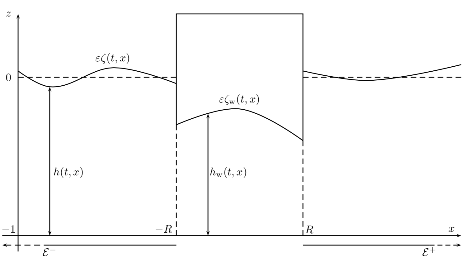 Figure 2
Peer Reviews
No public reviews on file for this paper yet. If you reviewed it on a platform where reviews are public (OpenReview, ICLR, NeurIPS, ICML), you can paste yours below so the community can read it here.
Videos
No videos yet. Explain this paper in a talk, walkthrough, or lecture? Add one.
Waves Interacting with a Partially Immersed Obstacle in the Boussinesq Regime
D. Bresch, D. Lannes, G. Métivier
Université Grenoble Alpes, Université Savoie Mont-Blanc et CNRS UMR5127, Batiment le chablais, 73376 Le Bourget du Lac Cedex, France
Institut de Mathématiques de Bordeaux
Université de Bordeaux et CNRS UMR 5251
351 Cours de la Libération
33405 Talence Cedex, France
[email protected], [email protected]
D. B is partially supported by the ANR-18-CE40-0027 Singflows and the ANR project Fraise, and D. L is partially sypported by the ANR-18-CE40-0027 Singflows, the Del Duca Fondation, the Conseil Régional d’Aquitaine and the ANR-17-CE40-0025 NABUCO.
Abstract
This paper is devoted to the derivation and mathematical analysis of a wave-structure interaction problem which can be reduced to a transmission problem for a Boussinesq system. Initial boundary value problems and transmission problems in dimension d= 1 for hyperbolic systems are well understood. However, for many applications, and especially for the description of surface water waves, dispersive perturbations of hyperbolic systems must be considered. We consider here a configuration where the motion of the waves is governed by a Boussinesq system (a dispersive perturbation of the hyperbolic nonlinear shallow water equations), and in the presence of a fixed partially immersed obstacle. We shall insist on the differences and similarities with respect to the standard hyperbolic case, and focus our attention on a new phenomenon, namely, the apparition of a dispersive boundary layer. In order to obtain existence and uniform bounds on the solutions over the relevant time scale, a control of this dispersive boundary layer and of the oscillations in time it generates is necessary. This analysis leads to a new notion of compatibility condition that is shown to coincide with the standard hyperbolic compatibility conditions when the dispersive parameter is set to zero. To the authors’ knowledge, this is the first time that these phenomena (likely to play a central role in the analysis of initial boundary value problems for dispersive perturbations of hyperbolic systems) are exhibited.
**Keywords: Wave-structure interaction, Boussinesq system, Free surface, Transmission problem, Local well posedness, Dispersive boundary layer, Oscillations in time, Compatibility conditions. **
1. Introduction
1.1. General setting
Free surface problems for various non-linear PDEs such as incompressible Euler and Navier-Stokes equations or reduced long-wave systems such as the nonlinear shallow water equations, the Boussinesq and Serre-Green-Nagdhi equations, have been strongly studied over the last decade: well-posedness, rigorous justification of asymptotic models, numerical simulations, etc. Recently, free surface interactions with floating or fixed structures have been addressed for instance in [19] where a new formulation of the water-waves problem was proposed in order to take into account the presence of a floating body. In this formulation, the pressure exerted by the fluid on the partially immersed body appears as the Lagrange multiplier associated to the constraint that under the floating object, the surface of the water coincides with the bottom of the object. This method was also implemented in [19] when the full water waves equations are replaced by simpler reduced asymptotic models such as the nonlinear shallow-water or Boussinesq equations. The resulting wave-structure models have been investigated mathematically when the fluid model is the nonlinear shallow water equations in the case of vertical lateral walls ([19] in the one dimensional case and [4] for two-dimensional, radially symmetric, configurations) as well as in the more delicate case of non vertical walls where the free dynamics of the contact points must be investigated [14]. An extension to the viscous nonlinear shallow water equations has also been recently derived and studied in [21]. On the numerical side, a discrete implementation of the above method was proposed in [19] while a relaxation method was implemented in [12, 13] for one dimensional shallow water equations with a floating object and a roof. Note finally that the resulting equations present an incompressible-compressible structure as in congestion phenomena; the interested reader is referred to [24, 11, 8, 25, 9] for instance.
Mathematically speaking, the interactions of an immersed object with waves described by the one-dimensional shallow water equations can be reduced to an hyperbolic (possibly free boundary) transmission problem for which a general theory has been developed in the wake of the study of the stability of shock waves [22, 23, 3] (see also [14] for a more specific general theory of one-dimensional free-boundary hyperbolic problems). If we want to consider more precise models for the propagations of the waves (e.g. Boussinesq or Serre-Green-Naghdi equations), the situation becomes more intricate because dispersive effects must be included and there is no general theory for transmission problems or even initial boundary value problems associated to such models. This is the situation we address in this paper where we consider waves described by a (dispersive) Boussinesq system interacting with a fixed partially immersed object with vertical lateral walls. The fact that the lateral walls are vertical simplify the analysis since the horizontal coordinates of the contact points between the object and the surface of the water are time independent. However, the discontinuity of the surface parametrization at the contact points makes the derivation of the model more complicated. This derivation is postponed to Section 2 where we show that the wave-structure interaction problem under consideration can be reduced to the following transmission problem where is the surface elevation above the rest state, the horizontal discharge, and where the bottom of the object is assumed to be the graph of a function above the interval (see Figure 1).
In dimensionless form, this system reads
[TABLE]
with and transmission conditions
[TABLE]
where and are defined as
[TABLE]
and where . The system is completed by the initial condition
[TABLE]
where is given. In this system is the so called amplitude parameter (the ratio of the typical amplitude of the waves over the depth at rest) and the shallowness parameter (the square of the ratio of the depth over the typical horizontal length). In the absence of floating object and in the Boussinesq regime (i.e. when and ) the equations (1.1) are known to furnish a good approximation to the water waves equations [18] for times of order .
Our main objective here is to prove the local in time well-posedness of the transmission problem (1.1)–(1.4) on the same time scale. To our knowledge, this is the first time that such a result is proved for a dispersive perturbation of a hyperbolic system. Indeed, the theory of initial boundary value problems for hyperbolic systems has been intensely investigated [22, 23, 3], but even in the one-dimensional case, there are very few results for dispersive perturbation of such systems, despite their ubiquitous nature : Boussinesq systems for water waves [18], internal waves [6], Euler-Korteweg system for liquid-vapour mixtures [2], elastic structures [17], etc. At best, one can find local existence results for initial boundary value problems but on an existence time which shrinks to zero as the dispersive parameter goes to zero [1, 5, 27, 20], falling far below the relevant time scale.
In order to reach this time scale, it is necessary to analyze and control the dispersive boundary layer that can be created at the boundary. In the particular case of the transmission problem (1.1)–(1.4), it is easy to construct local in time solutions (see Proposition 3.2 below). It is striking that these solutions are smooth if the data are smooth without having to impose compatibility conditions. This is in strong contrast with the hyperbolic case where it is well known that compatibility conditions of order are needed to obtain regularity. In our case, the dispersion automatically smoothes the solution by creating a dispersive boundary layer that compensates the possible discontinuities of the derivatives at the corner . In this boundary layer of typical size , the solution can behave quite wildly and standard techniques are unable to provide the necessary bounds to obtain an existence time independent of and (and a fortiori of order ). One therefore needs to analyze precisely the dispersive boundary layer. By doing so, it is possible to derive a new kind of compatibility conditions (that are estimates rather than equations) that need to be imposed to control the dispersive boundary layer. Interestingly enough, these new conditions degenerate to the standard hyperbolic compatibility conditions when the dispersion parameter is set to zero. We believe that our approach, based on the analysis of the dispersive boundary layer, is of general interest and should play a central role in the yet to develop theory of initial boundary value problems for dispersive perturbations of hyperbolic systems.
1.2. Organization of the paper
The outline of the article is as follows: In Section 2, we derive the transmission problem (1.1)-(1.4) from basic physical assumptions. In Section 3 we perform a change of variables that linearizes the transmission conditions and we rewrite the problem as an ODE which is locally well-posed with a blow-up criterion related to a maximal existence time which may depend of the small parameters and . The main objective is then to solve the system on the relevant time scale showing a uniform bound of the quantity appearing in the blow-up criterion. Our main result states that this is the case provided that some compatibility conditions are satisfied. Due to the presence of dispersive terms in the equations, these compatibility conditions differ from the standard hyperbolic compatibility conditions; they are analyzed in details in Section 4. We show in particular that if these new compatibility conditions are nonlocal, they can be approximated and replaced by local compatibility conditions that are easier to check. Section 5 is then dedicated to the uniform estimates of the time derivatives which rely on estimates for the linearized system and control of the commutators using modified Gagliardo-Nirenberg estimates in time and space that take into account the singularity of the multiplicative constants when the time interval is small. Section 6 is then dedicated to estimates of derivatives. As in the hyperbolic case, we use the equations, but this is now much trickier. Because of the dispersive term, instead of getting explicit expressions in terms of time derivatives and lower order derivatives, we are led to solve equations of the form and thus we have to control the rapid oscillations created by . Finally, Section 7 provides the proof of the main result, namely, the proof of Theorem 3.1, which is based on the proof of a uniform bound of the quantity appearing in the blow-up criterion.
1.3. Notations
- Throughout this paper, we use the following notations for the jump and average of a function across the floating object,
[TABLE]
- We also denote
[TABLE]
- We denote by the fluid domain, where
[TABLE]
-
We denote , and more generally for all .
-
We denote respectively by and the inverse of on with homogeneous Dirichlet and Neumann boundary data at , that is, and with
[TABLE]
2. Derivation of the model
2.1. Basic equations
We consider a wave-structure interaction problem consisting in describing the motion of waves at the surface of a one dimensional canal with a fixed floating obstacle. More precisely, we consider a shallow water configuration in which the waves are described, in dimensionless form, by the following Boussinesq system
[TABLE]
where is the surface elevation above the rest state, is the water depth, is the horizontal discharge (that is, the vertical integral of the horizontal component of the velocity field in the fluid domain), and is the value of the pressure at the surface. The parameters and are respectively called the nonlinear and shallowness parameters and defined as
[TABLE]
where is the typical amplitude of the waves, the depth at rest, and the typical horizontal scale. The weakly nonlinear regime in which the Boussinesq system is valid (see [18] for instance for the derivation and justification of this Boussinesq model) is characterized by the relation
[TABLE]
In this paper, we consider a fixed, partially immersed, object with vertical lateral walls located at and assume that the bottom of the object can be parameterized by a function on . We shall refer to as the interior domain and to as the exterior. The surface pressure is assumed to be given by the atmospheric pressure in the exterior domain, and by the (unknown) interior pressure on ,
[TABLE]
The pressure is therefore constrained on but not on , while this is the reverse for the surface elevation for which we impose
[TABLE]
that is, the surface of the water coincides with the (fixed) bottom of the obstacle on .
Finally, transmission conditions are provided at the contact points on the discharge and conservation of total energy is imposed,
[TABLE]
the latter condition is made more precise in the next section, where we show that it yields a jump condition on the interior pressure that allows to close the equations.
2.2. Derivation of a jump condition for the interior pressure from energy conservation
There are two different local conservation laws for the energy, one in the exterior region, and another one for the interior region.
- •
Local energy conservation in the exterior region. For the Boussinesq model (2.1) in the exterior region (i.e. with ), there is a local conservation of energy,
[TABLE]
with
[TABLE]
- •
Local energy conservation in the interior region. Let us first remark that from the first equation of (2.1) and (2.4), one gets that in the interior region. There exists therefore a function of time only such that
[TABLE]
The local conservation of energy reads
[TABLE]
with
[TABLE]
(recall that )
Since the object is fixed, the condition (2.6) is equivalent to saying that the total energy of the fluid should be constant, where
[TABLE]
Time differentiating and using (2.7) and (2.8), we impose therefore that
[TABLE]
and using the continuity condition (2.5) on , this yields the following jump condition for the interior pressure,
[TABLE]
setting in this relation, one recovers as expected the transmission condition obtained in [21] and [4] for the nonlinear shallow water equations.
2.3. Reformulation as a transmission problem
We show in this section that the wave-structure interaction problem under consideration can be reduced to the Boussinesq system (2.1) on the exterior domain ,
[TABLE]
together with transmission conditions relating the values of , (or derivatives of these quantities) at the contact points . As noticed in the previous section, one has in the interior region and on for some function depending only on time. From this and the continuity condition (2.5), we infer
[TABLE]
while the second equation of (2.1) implies that
[TABLE]
Integrating this relation on gives therefore
[TABLE]
Combining this with (2.9) provides a second transmission condition,
[TABLE]
We have therefore reduced the problem to the following transmission problem :
[TABLE]
with transmission conditions
[TABLE]
where and are defined as in §1.3 and where . The system is completed by the initial condition
[TABLE]
The rest of this paper is devoted to the mathematical analysis of this transmission problem. Note that a similar problem without the dispersive terms was considered in [19] in the case, in [4] in the -radial case and in [21] with viscosity. As we shall see, the situation here is drastically different as the dispersive boundary layer plays a central role and requires the development of new techniques.
3. Statement of the main result and sketch of the proof
3.1. Linearization of the transmission conditions
Note that the limiting problem is a hyperbolic transmission problem, and thus we expect to recover the main features of such problems. In particular, the initial data must satisfy compatibility conditions at the corners to get smooth solutions bounded on a uniform interval. But instead of being equations, these conditions are transformed into estimates, see below.
We also follow the general strategy of hyperbolic problems. The main part of the proof consists in proving uniform a priori estimates for smooth solutions. By construction, the system has a positive definite energy, providing good -types estimates. The next step is to look for estimates for tangential derivatives, that is here, time derivatives. Then, one get estimates for the derivatives, using the equation. The system for the time derivative is much nicer when the boundary conditions are made linear, and this is why we introduce the new unknown (instead of the elevation ) given by
[TABLE]
Note that the equivalence (written above) comes from the fact that we consider uniformly bounded quantities with respect to . Rewriting the problem in terms of and , one get the following nonlinear system
[TABLE]
with the linear transmission conditions
[TABLE]
and the initial condition
[TABLE]
where . The main objective of the paper is to prove the existence and uniqueness of solutions of the above system written in on a time interval such that is small enough under some compatibility conditions on the data. More precisely we will prove Theorem 3.1.
3.2. Reduction to an ODE
From now on, we restrict our attention to this new system (3.1)-(3.4). As a preliminary remark, we note that for , this system can be seen as an o.d.e. in a suitable Hilbert space. Introduce the inverse of with Dirichlet boundary conditions on each side of . First note that, for initial data which satisfy , the jump condition is equivalent to . Remark next that the second equation together with the jump condition is equivalent to
[TABLE]
with , and necessarily
[TABLE]
This implies that
[TABLE]
and therefore the second transmission condition (2.12) with is equivalent to
[TABLE]
that is
[TABLE]
Remark 3.1**.**
The fact that , which is the coefficient of the exponentially decaying term in (3.5), is given explicitly in terms of and is crucial for the ODE formulation of Proposition 3.1.
Hence we have proved the following result, where we recall that .
Proposition 3.1**.**
For such that and , the system (3.1)–(3.3) is equivalent to
[TABLE]
with
[TABLE]
and
[TABLE]
The smoothing properties of imply that the mapping is smooth from to itself for , so that the system (3.7) can be solved in this space, on an interval of time which depends on , see Proposition 3.2 below.
Remark 3.2**.**
In sharp contrast, the situation when is quite different. In this case, the equations can be written
[TABLE]
but is not anymore continuous on a fixed Sobolev space. More importantly, the boundary conditions
[TABLE]
are not propagated by the equations and, as usual for hyperbolic problems, the initial data must satisfy compatibility conditions to generate smooth solutions. This shows that (3.7) is a truly singular perturbation of (3.10), not only because one passes from bounded to unbounded operators, but also because of the boundary conditions, which are included in (3.7) and not in (3.10). **
The discussion above shows that the problem is reasonably well posed, but does not answer our objective : our goal is to solve (3.1)-(3.4) on an interval of time independent of and , and even more, of size . The first step is to use Cauchy Lipschitz theorem to prove local existence and derive a blow up criterion. We recall that .
Proposition 3.2**.**
For , consider initial data satisfying and . Then for all and , there is such that the system (3.1)–(3.4) has a unique solution in , which in addition belongs to . Moreover, if denotes the maximal existence time and , one has
[TABLE]
Proof.
Let denote the open subset of of the such that . Then is a smooth mapping from to and is a smooth mapping from to . For , maps to , so that the right hand side of (3.7) is a smooth mapping from to and the local existence of solutions of (3.7) follows for small enough. Next, when is smooth with , one has
[TABLE]
where is a continuous function on . This implies that for one has
[TABLE]
and therefore
[TABLE]
where
[TABLE]
and depends only on . Thus the solution satisfies
[TABLE]
implying that it be continued as long as remains bounded. The second part of the proposition follows. ∎
3.3. Compatibility conditions
Proposition 3.2 shows that in order to prove existence on a time interval (with independent of and a fortiori of size ), it is sufficient to prove a priori estimates which imply that remains uniformly bounded on . For that, we follow the lines of the analysis of hyperbolic equations, based on energy estimates. The -type estimates for are easy, and differentiating the equations in time, one obtains uniform estimates for in terms of , provided that the commutator terms can be controlled – see Proposition 5.2 below. However, such a control is useless if one cannot prove that the energy of the initial value of the time derivatives, namely, , is uniformly controlled in terms of standard Sobolev norms of the initial data . This is the issue addressed in this section.
We therefore seek to give conditions which ensure uniform bounds for the initial values of the . By (3.7), one can compute them inductively. Namely one has, when ,
[TABLE]
where
[TABLE]
and
[TABLE]
using systematically the notations , , . Indeed, and are non linear functions of for , so that (3.15) defines inductively for all in if .
The difficulty is that the relations (3.15) do not provide a uniform control (with respect to ) of the space derivatives in terms of space derivatives of the . Indeed, it follows from (3.15) and the definition (3.9) of that
[TABLE]
and it appears that both terms in the right-hand-side are of size (see §4.1 for details). The only way one can expect a uniform control of is that these two singular terms cancel one another. This is the case provided that the following compatibility conditions are satisfied, for some and all ,
[TABLE]
(roughly speaking, this means that the transmission conditions (3.2) and (3.2) are approximately satisfied by the up to ).
Remark 3.3**.**
Note that the are given by nonlinear functionals of involving and space derivatives, of total order at most . Therefore the conditions above are assumptions bearing only on the initials data . **
Under such conditions, it is possible to control the in Sobolev spaces, as shown in the following proposition whose proof is postponed to Section 4 for the sake of clarity.
Proposition 3.3**.**
Given and , there is a constant such that for all initial data and parameters in and satisfying
[TABLE]
[TABLE]
and the conditions (3.18) for , one has
[TABLE]
3.4. The main theorem
This being settled, our main result is the following. We recall that .
Theorem 3.1**.**
Let . Given , there is such that for all initial data and parameters and satisfying (3.19) and (3.20), and the compatibility conditions (3.18), there is a unique solution of (3.1)–(3.4), with .
Remark 3.4**.**
Recalling that and the assumption (2.2) of weak nonlinearity, namely, , the theorem provides an existence time which is which is the same as for the initial value (Cauchy) problem [26, 10].**
A drawback of Theorem 3.1 is that the compatibility conditions (3.18) are not easy to check, as the construction of the involve the nonlocal operator through the operator in (3.15). For instance, it is not clear to assess wether smooth initial data compactly supported away from the boundary satisfy the compatibility conditions (3.18). Taking advantage of the fact that the compatibility conditions (3.18) are estimates rather than equations, we derive here a set of approximate compatibility conditions that do not involve nonlocal operator (and therefore much easier to check) that are sufficient to obtain the result of Theorem 3.1.
We start by noticing that the second equation in (3.15) can be equivalently written
[TABLE]
where the inverse operator is associated to the boundary conditions
[TABLE]
A very naïve approximation of this formula is to replace the inverse by its Neumann expansion,
[TABLE]
Replacing the second equation in (3.15) by this approximation leads us to approximate by the defined through the induction relation
[TABLE]
with and defined as and but in terms of the rather than the . It is then natural to define the following approximate compatibility conditions: for some and all ,
[TABLE]
Remark 3.5**.**
Note that are given by nonlinear functionals of involving space derivatives, of total order at most . Therefore the conditions above are assumptions bearing only on the initials data . The difference with the compatibility condition (3.18) is that they do not involve nonlocal operators and just bear on the Taylor expansion of the initial data at the boundaries . They are therefore much easier to check; it is for instance trivial to verify that they are satisfied by smooth data compactly located away from the boundaries. **
The fact that the approximate compatibility conditions are sufficient to keep the results of Proposition 3.3 and Theorem 3.1 is not obvious, and the proof of the following corollary is left to Section 4 for the sake of clarity.
Corollary 3.1**.**
Under the same assumptions but replacing the compatibility condition (3.18) by its approximation (3.23), the results of Proposition 3.3 and Theorem 3.1 remain valid.
Remark 3.6**.**
Contrary to Theorem 3.1, Corollary 3.1 remains valid when . In this case, the transmission problem (3.1)-(3.4) is hyperbolic and the approximate compatibility conditions (3.23) are the standard hyperbolic compatibility conditions.
3.5. Outline of the proof
The outline of the paper is as follows: Section 4 is devoted to the derivation, analysis and approximation of the compatibility conditions. In section 5 we prove a priori uniform estimates for the time derivatives . This requires estimates for the linearized system (linear stability) and a control of the commutators for which we use a generalization of the space-time Gagliardo-Nirenberg estimates that makes explicit the singular dependence of the constants when the time interval is small.
In Section 6 we prove a priori uniform estimates for spatial derivatives. As in the hyperbolic case, we use the equations, but this is now much trickier. Because of the dispersive term, instead of getting explicit expressions in terms of time derivatives and lower order -derivatives, we are led to solve equations of the form
[TABLE]
and thus we have to control the rapid oscillations created by . Finally, the proof of the main Theorem 3.1 and of Corollary 3.1 in done in Section 7. It is based on a control of the blow up criterion provided by Proposition 3.2.
4. Compatible initial data
The goal of this section is to prove the uniform estimates of Proposition 3.3 under the compatibility conditions (3.18) and to show, as claimed in Corollary 3.1 that these uniform estimates remain true under the approximate compatibility conditions (3.18).
Throughout this section and we think of it as beeing small.
4.1. Analysis of the mapping
The key point for the derivation of the compatibility conditions is the analysis of the second, nonlocal, equation in the induction relation (3.15) that is used to construct the . We are therefore led to study the operator defined in (3.9) :
[TABLE]
This operator is well defined from to for . We look for estimates which make explicit the dependence on the parameter . When , we note that , and are uniformly bounded in . In particular,
[TABLE]
so that, with ,
[TABLE]
When , the difficulty is that and do not commute and that the layer is not uniformly bounded in . In this section, we show that compatibility conditions are needed in order to obtain uniform higher order Sobolev estimates on .
4.1.1. Higher order estimates of
As previously said, the -norms of have a singular dependence on . We make here this singular dependence explicit. Let denote the inverse of on with homogeneous Neumann conditions at .
Proposition 4.1**.**
For and , one has
[TABLE]
with
- •
* when is even*
- •
* when is odd,*
and
[TABLE]
Proof.
For all , the following identities hold,
[TABLE]
For the first identity, just notice that if , then solves on with boundary condition
[TABLE]
Thus and if . For the second identity, if , then solves with boundary condition , so that .
Hence, for ,
[TABLE]
Iterating these identities yields
[TABLE]
[TABLE]
proving the lemma. ∎
Thus the lack of commutation of with derivatives is encoded in the trace operators . It is convenient and more symmetric to introduce
[TABLE]
The following corollary tells us that if is a function of the form
[TABLE]
(as is by (4.1)), and if is bounded in then necessarily the singularities of (explicited in Proposition 4.1) and of the exponential layer must compensate. Moreover, the second point of the corollary shows that the global contribution of these singularities can be controlled by and .
Corollary 4.1**.**
For , there are constants and such that for all and and , the function satisfies
[TABLE]
and
[TABLE]
Proof.
Note that
[TABLE]
Hence, for , one has on
[TABLE]
Thus
[TABLE]
since . Taking , and noticing that
[TABLE]
(4.4) follows.
Moreover, . Therefore, for
[TABLE]
Note that, for , one has
[TABLE]
so that
[TABLE]
Together with (4.2) when , this implies that
[TABLE]
and the estimate (4.5) follows. ∎
4.1.2. Taylor expansions of and
In (4.1), the quantity is defined through an equation of the form (4.3) but with a scalar depending itself on . We are therefore led to study the Taylor expansion of terms of the form and, through Proposition 4.1, of . We start with a useful preliminary result. Introduce the non local trace operators
[TABLE]
from to , which satisfy
[TABLE]
Proposition 4.2**.**
For ,
[TABLE]
and for with ,
[TABLE]
Proof.
For , since one has
[TABLE]
Iterating this identity yields (4.6). In particular, if satisfies , then
[TABLE]
Thus if , then . ∎
Together with Proposition 4.1, this result can be used to obtain Taylor expansions of at in terms of .
Corollary 4.2**.**
Suppose that , with . Then, for ,
[TABLE]
where
- •
when is even then and
[TABLE]
- •
when is odd then and
[TABLE]
Proof.
The identity (4.7) follows immediately from Proposition 4.1 when is even. When is odd, one has
[TABLE]
Since is odd, , and Proposition 4.2 implies that
[TABLE]
and (4.7) follows. ∎
4.1.3. Compatibility conditions for the control of
From Corollary 4.2 we get in particular,
[TABLE]
where
[TABLE]
Thus
[TABLE]
so that
[TABLE]
with . A uniform control of can then be reduced to a control on the quantities and defined in the statement below.
Proposition 4.3**.**
For , there is a constant such that for all and the function with defined by (4.1) satisfies
[TABLE]
and
[TABLE]
where
[TABLE]
and
[TABLE]
Proof.
Apply Corollary 4.1 to and with
[TABLE]
Using (4.8) and noticing that , one has
[TABLE]
and
[TABLE]
Hence (4.9) and (4.10) follow from (4.4) and (4.5) respectively. ∎
Remark 4.1**.**
An important fact is that the operators are polynomial functions of , and thus smooth up to . In particular, at , they simplify to **
[TABLE]
In addition to the estimates of the proposition above, one has a precise description of the Taylor expansion of at .
Proposition 4.4**.**
For , there is a constant such that for all and the Taylor expansion at of with defined by (4.1) satisfies for
[TABLE]
Proof.
Using (4.3) with \sigma=\big{(}\rho+\delta^{2}\llbracket\partial_{x}R_{0}f\rrbracket\big{)}/(\alpha+2\delta), we get by using (4.7) that
[TABLE]
With (4.11) one can replace by up to an error of size , and next by up to additional error of size . Hence
[TABLE]
Now we use Corollary 4.2. When is even, and
[TABLE]
When is odd, {\mathcal{R}}^{\pm}_{l,k}f=\pm\Big{(}{\mathcal{D}}^{\pm}_{l}f\ +\ \sum_{l^{\prime}=l}^{k-1}(\pm\delta)^{l^{\prime}}\partial_{x}^{l^{\prime}}f_{|x=\pm R}\Big{)} and
[TABLE]
In both case, this proves (4.12). ∎
According to Proposition 4.4, one can approximate and . Together with Proposition 4.3, this implies the following Corollary that motivates the compatibility conditions (3.18).
Corollary 4.3**.**
For , there is a constant such that for all and the function with defined by (4.1) satisfies
[TABLE]
and
[TABLE]
where
[TABLE]
4.2. Proof of Proposition 3.3
We show here the uniform bounds of Proposition 3.3. Consider initial data and parameters and satisfying
[TABLE]
[TABLE]
for some given . Let us also introduce the notation
[TABLE]
which are defined through the induction relation (3.15). We also assume that the compatibility conditions (3.18) hold, that is,
[TABLE]
We will prove by induction on that there are constants which depend only on such that
[TABLE]
agreeing that the condition (4.16) is void at the final step .
When , (4.16) is our assumption. We assume that the estimates (4.25) and (4.26) are satisfied up to the order and prove them at the order .
The multiplicative properties of Sobolev spaces show that satisfies (4.16) for some . The fact that also satisfies (4.16) is a direct consequence of Corollary 4.3. This proves that (4.16) is satisfied for all . For the case , we first get as above that
[TABLE]
This give a bound for the norm of . Moreover, since and are uniformly bounded from to and respectively, one has
[TABLE]
which proves that (4.16) is also satisfied for all , and the proof of Proposition 3.3 is complete.
4.3. Approximate compatibility conditions
One issue with the compatibility conditions (3.18) is that they are nonlocal and very difficult to check. This is the reason why we show here that it is possible to replace them by the simpler compatibility conditions (3.23) that only involve the Taylor expansion of the initial condition at the boundaries . Moreover, as we shall see, as these new converge to the usual compatibility conditions of the hyperbolic boundary value problem. To explain that, we first recall briefly the analysis in the hyperbolic case.
4.3.1. Hyperbolic compatibility conditions
When (hyperbolic case), the induction is
[TABLE]
In this case, if , the are defined in only for . The compatibility conditions state that the boundary conditions are satisfied in the sense of Taylor expansion in time. They read and
[TABLE]
The -condition (4.18) bears only on the Taylor expansions at order of at . More precisely, for , let denote the coefficients of the Taylor expansion of . Then, for ,
[TABLE]
where and are polynomials of and of the for and . By (4.17)
[TABLE]
with leading term
[TABLE]
where is a smooth function of the coefficients with and . Hence by induction, this implies that for ,
[TABLE]
where is a smooth function of its arguments . Hence the compatibility conditions (4.18) which read
[TABLE]
are equations for which, thanks to (4.21), can be explicitly solved by induction on .
4.3.2. The dispersive case
When (dispersive case), the situation is quite different since is given by a nonlocal operator, so that the Taylor expansion of is not exactly a function of the sole Taylor expansions of the previous terms. However, when the approximate compatibility conditions (3.23) are satisfied up to order , this remains true approximately, so that the -th condition is equivalent to a condition on the Taylor expansions. Indeed, Proposition 4.4 tells us that it is then possible to make the approximation
[TABLE]
If we replace the nonlocal formula of (3.15) by this approximation, we are led to define a sequence of approximations of as follows:
[TABLE]
and we define
[TABLE]
where the operators and are defined as in (4.19) in the hyperbolic case, and next
[TABLE]
thus defining the for . Note that are polynomials of , the coefficients and so that they are well defined if in which case they coincide with the relation (4.20) obtained in the hyperbolic case.
We can consequently derive an approximation of the compatibility conditions (4.15), namely, that there exists such that
[TABLE]
We now show that the results of Proposition 3.3 remain true under these approximate compatibility conditions.
Proposition 4.5**.**
Given , there is a constant such that for all initial data and parameters and in satisfying (3.19) and (3.20), and the approximate compatibility conditions (4.24) for all , one has
[TABLE]
Remark 4.2**.**
The conditions (4.24) are explicit inequalities for the unknowns , which supplement the original jump condition assumed in (3.19). The functions , and are smooth functions of the and . When , one has and the conditions (4.24) reduce to (4.22). In particular, for small, the set of initial data satisfying (4.24) is a smooth variety.**
Remark 4.3**.**
If the initial data are supported away from the boundary , or more generally if their Taylor expansion at order vanish at , then the conditions (4.24) are satisfied. **
Proof.
Following the same path as in the proof of Proposition 3.3 but controlling in addition the size of the error , we will prove by induction on that there are constants which depend only on such that
[TABLE]
agreeing that the condition (4.26) is void at the final step .
When , (4.25) is our assumption, and (4.26) is trivial since .
We now assume that the estimates (4.25) and (4.26) are satisfied up to the order and prove them at the order .
The multiplicative properties of Sobolev spaces immediately imply the following estimates
[TABLE]
where is constant which depends only on . In particular, this shows that satisfies (4.25) for some .
With notations as in (4.19), the Taylor expansions at of and are given by functions and which are polynomials of and with and . The induction hypothesis (4.25) implies that the coefficients for and remain in a ball of radius , on which the derivatives of the functions and are bounded. Hence comparing (4.19) and (4.23) implies that
[TABLE]
and using the induction hypothesis (4.26), one obtains that for ,
[TABLE]
In particular, this shows that satisfies (4.26). By Proposition 4.4 and (4.24) we get that also satisfies (4.26) and that a similar upper bounds also holds for . The compatibility condition (4.15) is therefore a direct consequence of its approximate version (4.24). Hence, we can use Proposition 4.3 to obtain (4.25). By induction, we have then proved that (4.25) holds for . For , one gets the result as in the proof of Proposition 3.3. ∎
4.4. An additional bound
By Proposition 4.5, we have a control of in , and thus of the boundary values for . The proof of the main theorem uses an energy estimate of which requires and additional control of . When if follows form the estimate above. However, we need to control the time derivatives up to , and we now provide the needed control of .
By Proposition 3.2, we know that for initial data in satisfying and , there is a unique solution for some . Using the o.d.e formulation (3.7), we see that is indeed , so that the are defined for all and belong to . So the quantities are well defined. Moreover, by (3.6) we know that on ,
[TABLE]
Hence, for all ,
[TABLE]
In particular,
[TABLE]
Under the assumptions of Proposition 4.5, we have a uniform control of the in for , and hence of the in . Hence we have the following additional estimate.
Proposition 4.6**.**
Under the assumptions of Proposition 4.5, there is a constant such that for all ,
[TABLE]
5. Uniform estimates of time derivatives
The goal of this section is to prove the a priori estimates for the which are stated in Proposition 5.2 below. From the beginning, we know that there is a conserved energy for the nonlinear system. The system obtained for time derivatives is a linearized version of of (3.1)–(3.3), and we first prove energy estimates for it. Controlling the commutators, they will imply estimates for the time derivatives of the solution.
Notation 1**.**
Given ”constants” , we denote by or a function of these constants, which may change from one line to another. It is assumed that the dependence of these functions on their arguments is nondecreasing and that they are independent of and in .
5.1. -bounds
Consider the following linearized version of (3.1)–(3.3) around some reference state , with non-homogeneous source terms
[TABLE]
with transmission conditions
[TABLE]
We derive here an a priori bound for the total energy associated to this linear system,
[TABLE]
where represents the (linearized) energy of the fluid under the object (up to terms that are constant since the solid is not moving), while corresponds to the full (linearized) energy of the fluid in the exterior domain,
[TABLE]
Proposition 5.1**.**
Let and assume that satisfies and that there are constants and such that
[TABLE]
Then there exists such that the solutions of (5.1)–(5.3) satisfy for
[TABLE]
Proof.
Multiplying the first equation of (5.1) by and the second by , one gets
[TABLE]
with
[TABLE]
Integrating over , we then get
[TABLE]
Because , (5.3) implies that
[TABLE]
Therefore
[TABLE]
[TABLE]
Estimating by , the result follows from Gronwall’s lemma. ∎
5.2. Nonlinear estimates
In preparation for the control of the commutators in the energy estimates for the times derivatives, we first recall some Gagliardo-Nirenberg inequalities.
Lemma 5.1**.**
Let such that for some . Then, for and such that , there is a constant such that
[TABLE]
Combined with Hölder’s estimates to interpolate between and , this implies that for
[TABLE]
Functions defined in can be extended to by multiple reflections which preserve, up to numerical constants, the norms of the functions and their derivatives. Thus the estimates above remain true, with new constants for functions supported in . For functions supported in , one can proceed similarly when using extension operators, but when , one has to argue differently because the extension operators are not uniformly bounded when . When and , one can define the trace of at for . If
[TABLE]
the extension of by [math] for belongs to and and the estimates above are satisfied. Suppose more generally that
[TABLE]
Let
[TABLE]
Then and for . Because for , one has
[TABLE]
The difference satisfies (5.7) and we can estimate the norm of using (5.6), as explained above. Adding up, this implies that
[TABLE]
Using this estimate when and (5.6) when , we have proved the following estimates which are valid in both cases.
Lemma 5.2**.**
For all , and , there is such that for all with satisfying (5.8), one has
[TABLE]
where
[TABLE]
5.3. Bounds on the time derivatives of the solution
Let be a solution of the transmission problem (3.1)–(3.3). Let also . Differentiating the equations in time yields
[TABLE]
with transmission conditions
[TABLE]
and
[TABLE]
The following two lemmas provide some control on the source terms and .
Lemma 5.3**.**
For one has for all :
[TABLE]
with given by .
Proof.
Note that is a linear combination of terms
[TABLE]
with , and . We apply Lemma 5.2 to and , to estimate in with exponents such that and . Note that such a choice is possible because . This implies that
[TABLE]
and adding such estimates one gets the result. ∎
Lemma 5.4**.**
For one has for all :
[TABLE]
with now
[TABLE]
Proof.
Using the first equation of (5.9) one can replace by in (5.12). Using the representation of the given above, we see that is a linear combinations of two types of terms: first we have
[TABLE]
with with and second
[TABLE]
with . The estimate follows from Lemma 5.2 applied to and , the norm of the coefficients depending only on . ∎
We can now estimate the norm of applying Proposition 5.1 to (5.9). Let
[TABLE]
Proposition 5.2**.**
Let and , and assume that is a solution of (3.1) such that there are constants and such that
[TABLE]
Then there are constants and such that
[TABLE]
with is given by (5.13) (with ).
Proof.
By (5.5), one has
[TABLE]
with depends on and . By the equation we can estimate
[TABLE]
and thus . Using the lemmas above to estimate the norms of and and the inequalities
[TABLE]
with , , one obtains that
[TABLE]
The proposition follows by Gronwall’s lemma. ∎
6. Estimates of -derivatives
The next step is to prove estimates for and that are required in the statement of Proposition 5.2. They follow from estimates, that is from estimates of . The quantity is explicitly given by the first equation but the control of is more involved because of the term in the second equation. We will derive a second order o.d.e. for , and get estimates from it. It turns out that to obtain closed estimates we need to control up to .
6.1. Estimates for
We show here that the -norm (and therefore the -norm) of can be controlled up to in terms of the energy norm, the initial data, and the norm of and .
Lemma 6.1**.**
Let and , and suppose that where is a solution of (3.1) such that there are constants and such that
[TABLE]
for some positive constants and with given by (5.15). Then there are constant and such that
[TABLE]
and, for ,
[TABLE]
where is defined at (5.13).
Proof.
The first estimate is immediate from the equation:
[TABLE]
The norm of is controlled by . Thus, to prove the second inequality, it is sufficient to prove an estimate of . By (5.9)
[TABLE]
The -norm of the first term is of order . For the second we use that
[TABLE]
Using Lemma 5.2 one obtains that for ,
[TABLE]
Hence
[TABLE]
Noticing that , the lemma follows. ∎
6.2. A linear o.d.e. for
In the second equation of (3.1) we use the first one to replace by , obtaining that
[TABLE]
We reorganize this equation using that
[TABLE]
with so that
[TABLE]
and appears as a solution of the equation
[TABLE]
where
[TABLE]
and
[TABLE]
We differentiate (6.1) in time (alternately, on can start from (5.9)) to obtain an equation for . One has
[TABLE]
Thus
[TABLE]
with
[TABLE]
[TABLE]
and
[TABLE]
where the are numerical constants of no importance.
For our purposes, we are looking at solutions which remain uniformly bounded (with respect to and ) for times of order . Since the ODE is singular because of the coefficient in front of the higher order term, a direct application of Duhamel’s formula requires that the right-hand-side is of order in order for the solution to be uniformly bounded solution on the time scale. A refined study, that takes advantage of the oscillating nature of the solutions of the homogeneous equation, is required to handle the contribution of and even source terms. This is shown in the next subsection.
6.3. The basic estimate for the o.d.e
We start with a simplified equation
[TABLE]
assuming that the coefficient satisfies on
[TABLE]
We are looking for estimates of in and . To avoid repetitions we make a unique statement, using the notation for or .
Lemma 6.2**.**
Given constants and , there are and such that for , in , satisfying (6.6) and for , and , the solutions to the o.d.e. (6.5) satisfy the following estimate for all ,
[TABLE]
with
[TABLE]
Proof when .
The natural energy is
[TABLE]
which satisfies
[TABLE]
where .
Multiplying the equation by and integrating over yields
[TABLE]
where . Because , the first integral in the right hand side can be estimated by
[TABLE]
In order to prove the lemma, we note that is the sum of the three solutions obtained first when , second when and the initial conditions vanish and third when and the initial conditions vanish. We prove the estimate in each case separately.
– **Case a) : ** . In this case, the second integral is
[TABLE]
Using this last estimate with (6.10) and (6.11) and Gronwall’s lemma, this implies the estimate (6.7) with .
– **Case b) : ** and . Then
[TABLE]
The second term satisfies
[TABLE]
Moreover for all
[TABLE]
and
[TABLE]
Therefore
[TABLE]
We use this estimate together with (6.11) and (6.10). Choosing a small fraction of to absorb the term in from the left to the right, and using Gronwall’s lemma, the estimate (6.7) follows.
– **Case c) : ** and . Then
[TABLE]
Let us first bound as follows
[TABLE]
The difference with the previous case is that there is no in so we have to treat the second term differently. Using the equation, we note that
[TABLE]
The first term is
[TABLE]
In the second term, we integrate by parts :
[TABLE]
In the first integral, we integrate by parts again and get that
[TABLE]
The integrals over are dominated by
[TABLE]
The integrals over at time are estimated by
[TABLE]
We can therefore conclude using (6.12)–(6.18)
[TABLE]
Gathering the estimates obtained for the three cases, and choosing small enough, we obtain that there is and such that
[TABLE]
Gronwall’s lemma implies the result. ∎
Proof when .
The proof above applies for each fixed ; taking the supremum in instead of integrating over therefore yields the result. ∎
The complete equation (6.3) reads
[TABLE]
and can be seen as a perturbation of (6.5).
Lemma 6.3**.**
Given constants , and , there are , and a smooth nondecreasing function with such that for , in , satisfying (6.6) and satisfying
[TABLE]
and for , and , the solutions to the o.d.e (6.19) satisfies estimate
[TABLE]
with as in (6.8).
Proof.
We put the perturbation on the right hand side, and use the estimate (6.7). When , this terms contributes to the right hand side of the estimate adding a term dominated by
[TABLE]
which is absorbed from the right to the left by Gronwall’s lemma, implying (6.21). When , there is a similar estimate for each fixed , and one concludes taking sup as in the proof of the previous lemma. ∎
6.4. estimate of
We turn back to (3.1) and consider a solution such that
[TABLE]
With and coefficients given by (6.2), the conditions (6.6) and (6.20) are satisfied, with a constant, and Lemma 6.3 can be used to provide a bound on .
Lemma 6.4**.**
There are and and a nondecreasing function with such that if is a solution of (3.1) satisfying (6.22), then satisfies
[TABLE]
where
[TABLE]
Proof.
Recalling that satisfies the o.d.e (6.1), we use Lemma 6.3 with remarking that there is no in the right and side. Then we just have to control time derivatives of and .
Note that for one has
[TABLE]
Similarly,
[TABLE]
and
[TABLE]
The estimate follows then using Lemma 6.3. ∎
6.5. estimates of
Our goal here is to give an estimate of
[TABLE]
In order to use Lemma 5.2 we also introduce
[TABLE]
As usual, denotes a nondecreasing function such that .
Lemma 6.5**.**
There are constants , and where are defined by (6.22), (6.26) and a nondecreasing function with such that if is a solution of (3.1) satisfying (6.22) and (6.23), then
[TABLE]
where is given by (6.25).
Proof.
We apply Lemma 6.3 with to the equation (6.3). With and coefficients given by (6.4), the conditions (6.6) and (6.20) are satisfied for some if (6.22) holds. Thus we have an estimate (6.21) for with source term , to which contribute the three terms in the right hand side of (6.3).
– a) The first contributor is . Thus, for , one has
[TABLE]
Moreover, the integrated terms are . Hence the total contribution of satisfies
[TABLE]
– **b) ** The second contributor is \psi_{(j)}=2\partial_{t}^{j}\big{(}q(1+\varepsilon c^{\prime})\partial_{t}\theta\big{)}. Expanding the derivatives, we obtain a sum of terms of the form (5.14) and Lemma 5.2 implies that for ,
[TABLE]
where is given by (6.26).
In addition, we note that all the terms for belong to with norm at most . Therefore
[TABLE]
Hence the total contribution of satisfies
[TABLE]
– **c) ** The third contributor is a linear combination of terms
[TABLE]
with , and . First we use Lemma 5.2 to control norms of . For , there holds
[TABLE]
Let us consider two cases and then to control terms involving .
Case : By Lemma 5.2 applied to , one has for ,
[TABLE]
Then recalling that
[TABLE]
so that one can find indices and such that
[TABLE]
and
[TABLE]
Thus,
[TABLE]
If , it remains terms of the form
[TABLE]
We apply Lemma 5.2 to : for ,
[TABLE]
Remarking that
[TABLE]
we can choose indices and such that , , and and in this case we obtain that
[TABLE]
Summing up, this shows that the contribution of satisfies
[TABLE]
Adding up, we have obtained an estimate of . In appears a term
[TABLE]
which is absorbed to the left by Gronwall’s lemma. The other terms are all controlled by the right hand side of (6.27). ∎
7. Proof of the main Theorem
We prove here Theorem 3.1. Using Proposition 4.5 instead of Proposition 3.3, one easily deduces Corollary 3.1. We consider initial data , , satisfying for some ,
[TABLE]
and the compatibility condition (3.18) which we recall here for the reader’s convenience,
[TABLE]
By Proposition 3.2, we know that the solution belongs to on a maximal interval of time , but with , possibly small. The following proposition shows that this maximal interval of time is at least of order O\big{(}(\varepsilon+\delta^{2})^{-1}\big{)}.
Proposition 7.1**.**
Let . Given a constant , and an initial data satisfying (7.1) and (7.2), there is such that . Moreover, there are constants () such that for one has
[TABLE]
where , are respectively given by (5.15) and (6.25).
Proof.
We proceed in several steps.
– **a) ** Introduce for
[TABLE]
Lemma 7.1**.**
There is such that if , and , then
[TABLE]
Proof.
By Taylor expansion, there is such that
[TABLE]
∎
– **b) ** Consider the energy defined in (5.15). By Proposition 4.5 and Proposition 4.6, we know that there is a constant such that the initial energy satisfies
[TABLE]
where and are respectively given by (6.26) and (5.15). Proposition 5.2 therefore implies the following estimate.
Lemma 7.2**.**
There are and such that if , and , then
[TABLE]
The important point is that may depend on , but not .
– **c) ** Introduce
[TABLE]
We apply Lemma 6.4 noticing that by Proposition 4.5, is controlled by (choosing a larger if necessary in (7.5)).
Lemma 7.3**.**
There are , and such that if , and , then
[TABLE]
– d) We now apply Lemma 6.5 to bound the energy defined at (6.25). The initial value , as well as the constant defined in (6.26) are controlled by (choosing a larger if necessary in (7.5)). Using the bound (7.6) and demanding for instance that
[TABLE]
one obtains that there are and such that if ,
[TABLE]
Combining with (7.7), this implies the following lemma.
Lemma 7.4**.**
There are and such that if , and , then
[TABLE]
– **e) ** We note now that is controlled by and . Indeed, Lemma 6.1 and the Sobolev imbedding imply that
[TABLE]
if and is small enough. We now use the interpolation estimate
[TABLE]
which applied to for , implies that
[TABLE]
Hence we have proved that
[TABLE]
Inserting this estimate in (7.8) and choosing small, we have proved the following result.
Lemma 7.5**.**
If , there are constants and such that if , and ,
[TABLE]
Again, the important point is that may depend on , but not .
– **f) ** To close the loop, we note that Sobolev’s imbedding theorem implies that if
[TABLE]
– **g) **End of the proof. In the previous steps, we have constructed constants which depend only on given in the assumptions. We note also that
[TABLE]
Increasing if necessary, we can assume that and we now choose such that
[TABLE]
For instance we can choose . For this , there are such that the estimates (7.5) …(7.10) are satisfied for , as long as , and then, by (7.10) . Note that, given the choice of , is a function .
Since , this implies by continuity of that
[TABLE]
In particular the estimates (7.5) …(7.9) are satisfied if . By Lemma 6.1, we see that is bounded on this interval. Moreover, the -norm of , and thus its norm, is bounded by and . Therefore, there is such that for ,
[TABLE]
Therefore, the blow-up criterion of Proposition 3.2 implies that and the proof of the Proposition 7.1 is now complete. ∎
Theorem 3.1 is then a direct consequence of Proposition 3.2.
The reference list from the paper itself. Each links out to its DOI / PubMed record.
- 1[1] D. Antonopoulos, V. Dougalis, D. Mitsotakis , Initial-boundary-value problems for the bona-smith family of boussinesq systems , Advances Diff. Equations 14 (2009), 27-53.
- 2[2] S. Benzoni-Gavage, R. Danchin, S. Descombes , On the well-posedness for the Euler-Korteweg model in several space dimensions , Indiana University Mathematics Journal, (2007), 1499-1579.
- 3[3] S. Benzoni, D. Serre. Multi-dimensional hyperbolic partial differential equations: First-order systems and applications. Oxford Science Publications 2006.
- 4[4] E. Bocchi , Floating structures in shallow water: local well-posedness in the axisymmetric case, A r x i v 1802.07643 𝐴 𝑟 𝑥 𝑖 𝑣 1802.07643 Arxiv 1802.07643 .
- 5[5] J. Bona, M. Chen , A Boussinesq system for two-way propagation of nonlinear dispersive waves , Physica D 116 (1998), 191-224.
- 6[6] J. L. Bona, D. Lannes, J.-C. Saut , Asymptotic models for internal waves , J. Math. Pures Appl. 89 (2008), 538-566.
- 7[7] U. Bosi, A.P. Engsig-Karup, C. Eskilsson, and M. Ricchiuto , An efficient unified spectral element Boussinesq model for a point absorber, Eur. Workshop on High Order Nonlinear Numerical Methods for Evolutionary PD Es (HONOM), Stuttgart (Germany), 2017.
- 8[8] C. Bourdarias, M. Ersoy, S. Gerbi , A mathematical model for unsteady mixed flows in closed water pipes , Sci. China Math. 55 (2012), 221-244.