Task-based Augmented Contour Trees with Fibonacci Heaps
Charles Gueunet (LIP6), P. Fortin (LLR), J Jomier, J Tierny

TL;DR
This paper introduces a parallel algorithm for computing augmented contour trees efficiently on multi-core systems, enabling advanced data segmentation tasks with improved scalability and performance.
Contribution
It re-formulates the traditional contour tree algorithm into independent local tasks using Fibonacci heaps, allowing efficient parallel computation of augmented trees.
Findings
Superior runtime performance compared to existing methods
Scalability demonstrated on common workstations
Effective application in data segmentation
Abstract
This paper presents a new algorithm for the fast, shared memory, multi-core computation of augmented contour trees on triangulations. In contrast to most existing parallel algorithms our technique computes augmented trees, enabling the full extent of contour tree based applications including data segmentation. Our approach completely revisits the traditional, sequential contour tree algorithm to re-formulate all the steps of the computation as a set of independent local tasks. This includes a new computation procedure based on Fibonacci heaps for the join and split trees, two intermediate data structures used to compute the contour tree, whose constructions are efficiently carried out concurrently thanks to the dynamic scheduling of task parallelism. We also introduce a new parallel algorithm for the combination of these two trees into the output global contour tree. Overall, this…
Click any figure to enlarge with its caption.
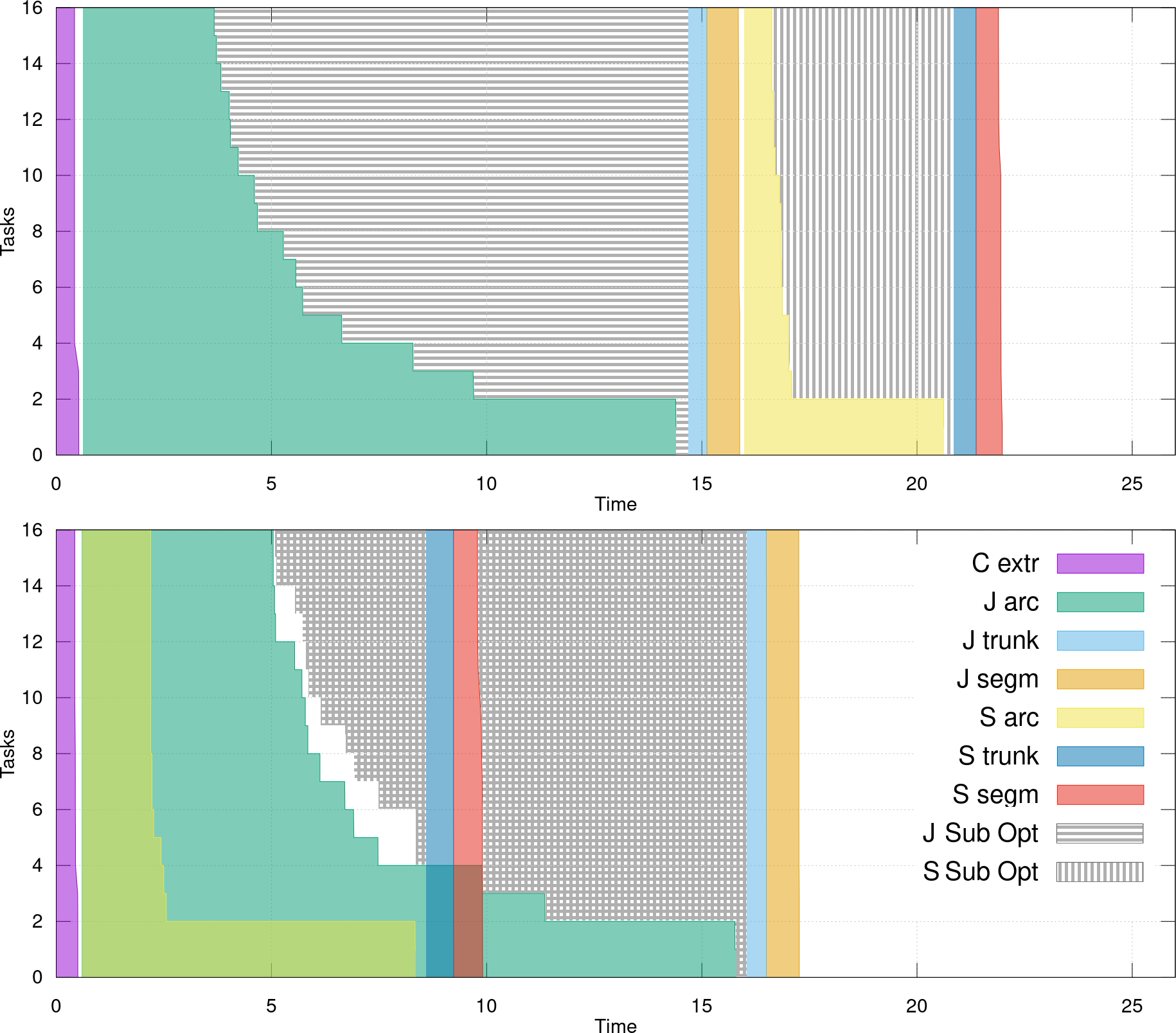 Figure 1
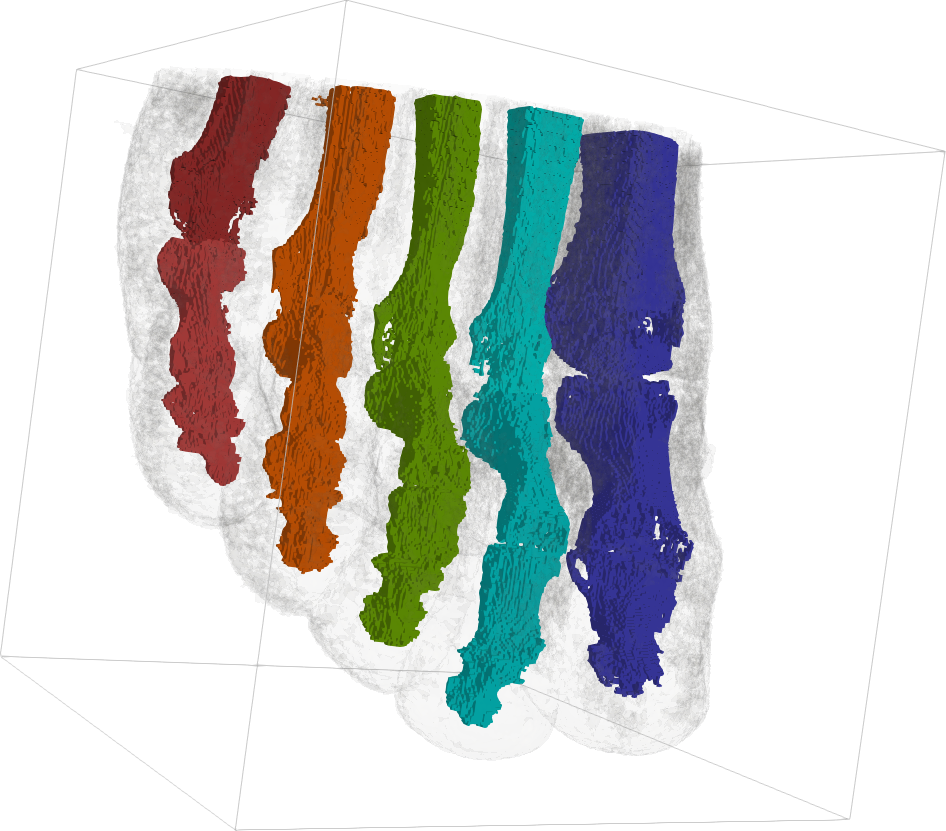 Figure 2
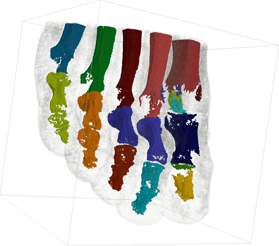 Figure 3
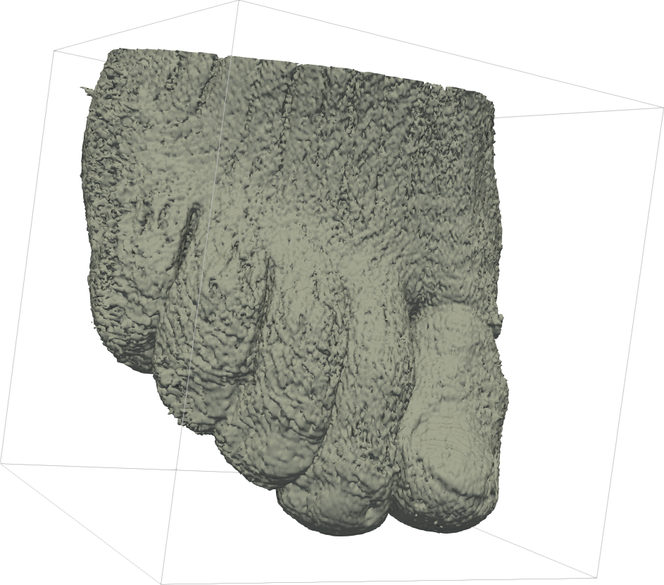 Figure 4
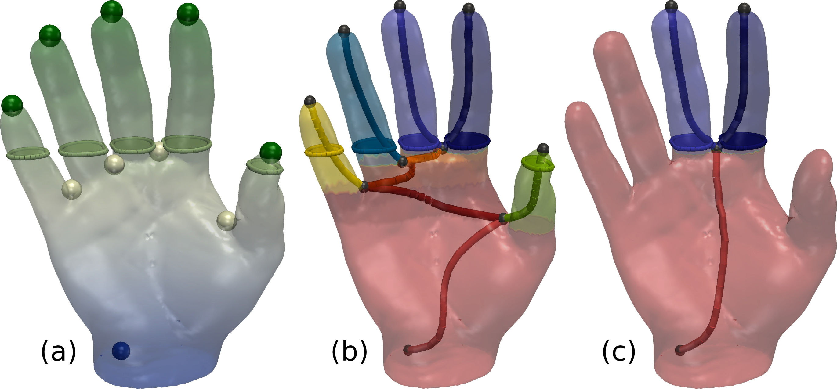 Figure 5
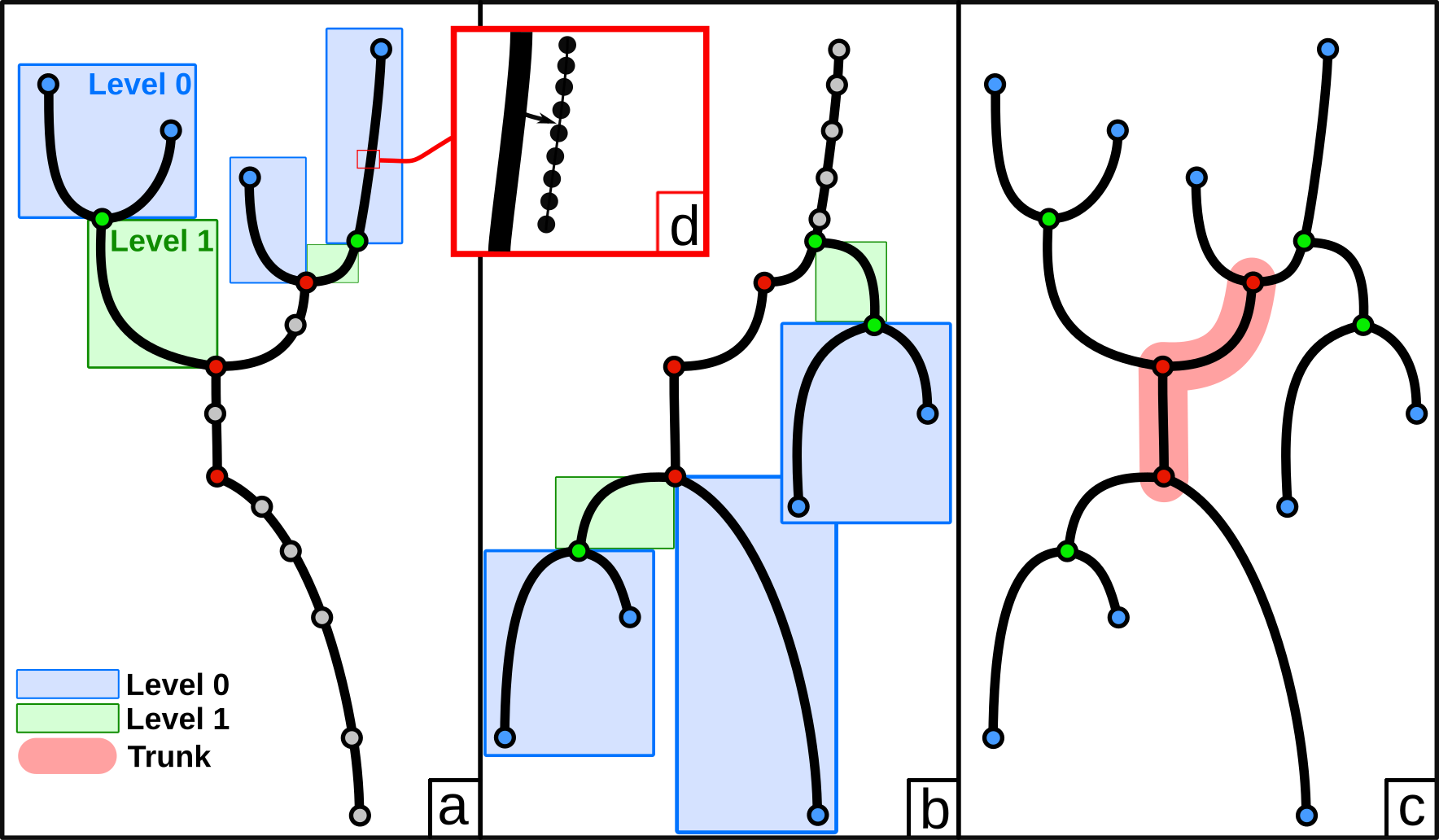 Figure 6
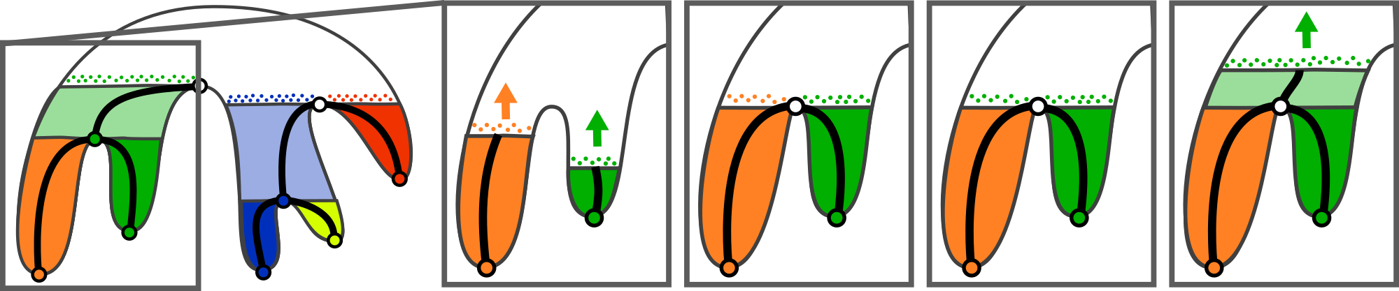 Figure 7
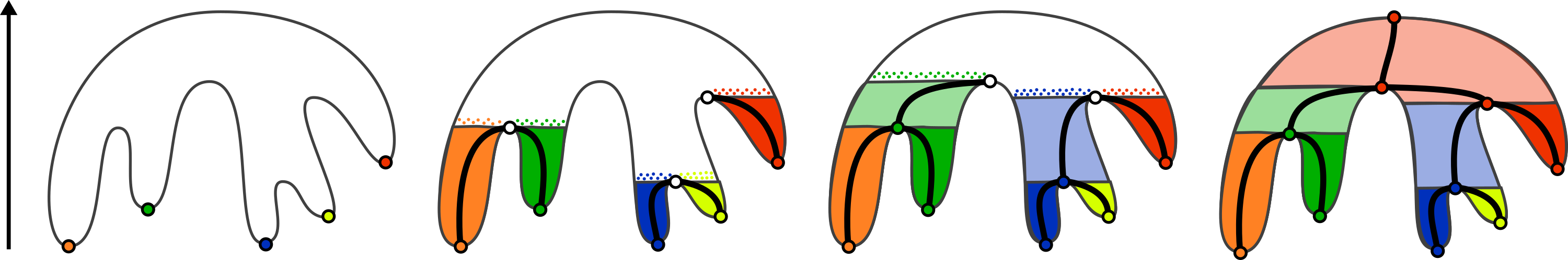 Figure 8
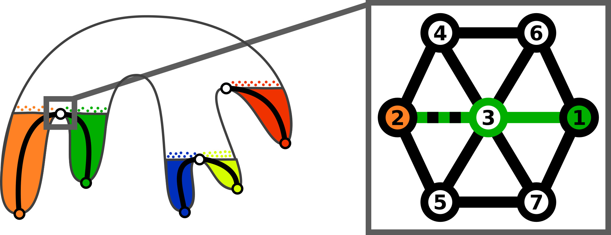 Figure 9
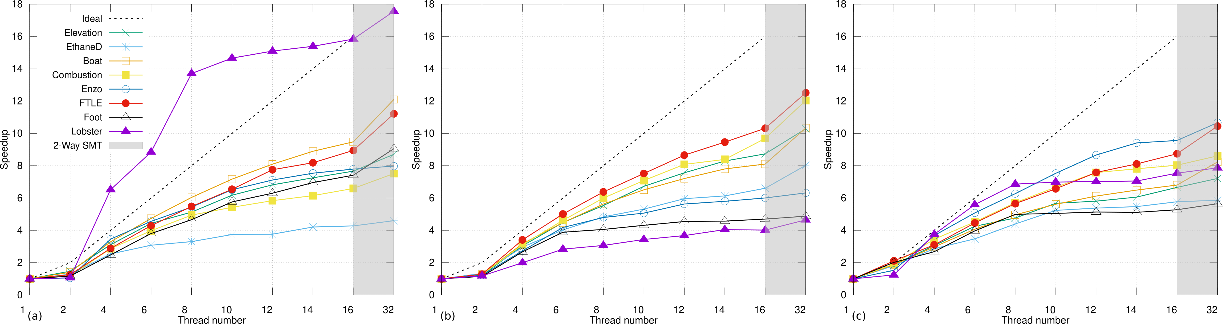 Figure 10
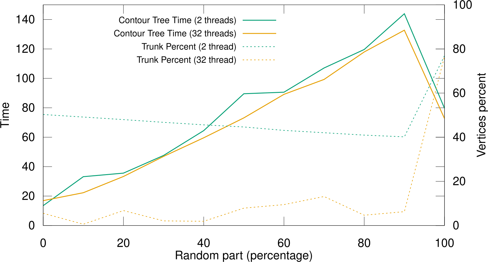 Figure 11
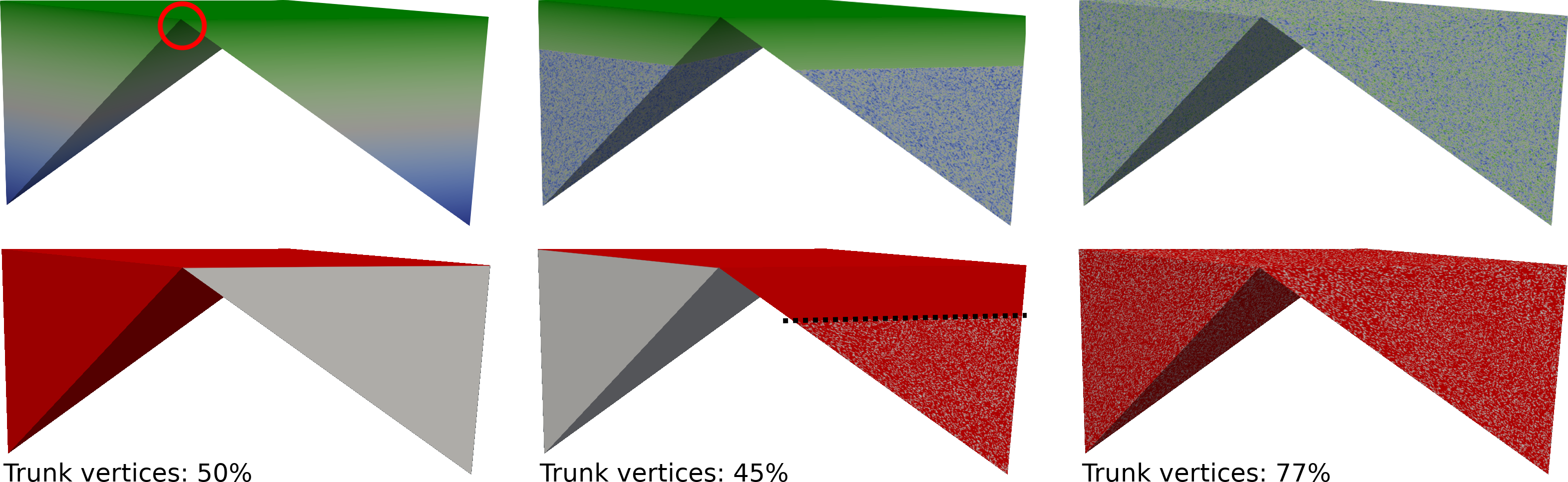 Figure 12
| Sequential | Parallel (32 threads on 16 cores) | |||||||
| Leaf | Arc | Trunk | ||||||
| Data set | Overall | Sort | search | growth | growth | Overall | Speedup | |
| 1 | 11.44 | 0.84 | 0.14 | 0 | 0.20 | 1.19 | 9.57 | |
| Elevation | 1 | 18.71 | 0.84 | 0.65 | 0 | 0.20 | 1.71 | 10.89 |
| 17 | 35.13 | 1.31 | 0.28 | 5.16 | 0.62 | 7.38 | 4.75 | |
| Ethane Diol | 19 | 30.79 | 1.31 | 0.30 | 2.58 | 0.62 | 4.82 | 6.38 |
| 5,426 | 29.72 | 1.24 | 0.24 | 0.07 | 0.64 | 2.21 | 13.41 | |
| Boat | 1,715 | 29.59 | 1.24 | 0.40 | 0.59 | 0.63 | 2.88 | 10.27 |
| 26,981 | 37.20 | 1.23 | 0.37 | 3.04 | 0.61 | 5.27 | 7.04 | |
| Combustion | 23,606 | 32.38 | 1.23 | 0.29 | 0.53 | 0.63 | 2.69 | 12.03 |
| 96,061 | 129.62 | 1.35 | 0.36 | 12.79 | 0.69 | 15.20 | 8.52 | |
| Enzo | 115,287 | 43.23 | 1.35 | 0.36 | 4.06 | 0.77 | 6.55 | 6.59 |
| 147,748 | 31.21 | 1.28 | 0.37 | 0.42 | 0.70 | 2.78 | 11.19 | |
| Ftle | 202,865 | 35.85 | 1.28 | 0.31 | 0.60 | 0.70 | 2.91 | 12.31 |
| 241,841 | 25.06 | 1.04 | 0.26 | 0.80 | 0.55 | 2.67 | 9.38 | |
| Foot | 286,654 | 48.59 | 1.06 | 0.55 | 7.82 | 0.53 | 9.97 | 4.87 |
| 472,862 | 96.34 | 1.07 | 0.30 | 3.59 | 0.73 | 5.71 | 16.86 | |
| Lobster | 490,236 | 36.64 | 1.05 | 0.62 | 5.45 | 0.78 | 7.91 | 4.62 |
| Sequential | Parallel | |||
| Data set | Arc growth | Trunk | Arc growth | Trunk |
| Elevation | 0 | 113,217,189 | 0 | 468,537,720 |
| Ethane Diol | 472,861 | 13,862,083 | 1,003,125 | 202,175,593 |
| Boat | 446,981 | 13,941,128 | 933,281 | 193,274,082 |
| Combustion | 453,784 | 14,104,274 | 1,416,082 | 196,810,503 |
| Enzo | 344,129 | 11,170,128 | 2,514,479 | 138,666,543 |
| Ftle | 594,694 | 14,007,046 | 3,198,233 | 154,453,693 |
| Foot | 447,270 | 27,073,541 | 2,257,674 | 182,413,262 |
| Lobster | 734,705 | 19,884,438 | 2,534,264 | 135,125,845 |
| Data set | Min | Max | Range | Average | Std. dev |
| Elevation | 1.17 | 1.19 | 0.02 | 1.18 | 0.01 |
| Ethane Diol | 7.37 | 8.67 | 1.29 | 8.00 | 0.42 |
| Boat | 2.11 | 2.21 | 0.09 | 2.14 | 0.02 |
| Combustion | 4.61 | 5.27 | 0.65 | 4.89 | 0.17 |
| Enzo | 14.44 | 15.82 | 1.38 | 15.29 | 0.53 |
| Ftle | 2.75 | 2.82 | 0.07 | 2.78 | 0.02 |
| Foot | 2.63 | 2.70 | 0.07 | 2.67 | 0.02 |
| Lobster | 5.36 | 5.71 | 0.34 | 5.53 | 0.13 |
| Data set | LT | CF | FTM | FTC | LT / FTC | CF / FTC | FTM / FTC |
| Elevation | 5.81 | 7.70 | 3.41 | 1.44 | 4.01 | 5.31 | 2.35 |
| Ethane Diol | 11.59 | 17.75 | 7.21 | 3.61 | 3.20 | 4.91 | 1.99 |
| Boat | 11.84 | 17.11 | 7.81 | 3.06 | 3.86 | 5.57 | 2.54 |
| Combustion | 11.65 | 16.87 | 7.96 | 4.05 | 2.87 | 4.15 | 1.96 |
| Enzo | 14.33 | 17.99 | 18.00 | 13.62 | 1.05 | 1.32 | 1.32 |
| Ftle | 11.32 | 15.62 | 7.24 | 3.55 | 3.18 | 4.39 | 2.04 |
| Foot | 9.45 | 12.72 | 5.94 | 3.20 | 2.95 | 3.97 | 1.85 |
| Lobster | 11.65 | 14.80 | 14.20 | 10.05 | 1.15 | 1.47 | 1.41 |
| Data set | LT | CF | FTM | FTC | LT / FTC | CF / FTC | FTM / FTC |
| Elevation | 5.00 | 2.33 | 0.35 | 0.18 | 27.19 | 12.67 | 1.95 |
| Ethane Diol | 8.95 | 4.54 | 1.24 | 0.85 | 10.52 | 5.33 | 1.46 |
| Boat | 8.24 | 4.40 | 0.61 | 0.29 | 28.02 | 14.96 | 2.09 |
| Combustion | 7.96 | 5.82 | 0.86 | 0.54 | 14.62 | 10.69 | 1.59 |
| Enzo | 12.18 | 8.92 | 1.91 | 1.60 | 7.60 | 5.56 | 1.19 |
| Ftle | 8.19 | 4.98 | 0.97 | 0.54 | 15.12 | 9.19 | 1.80 |
| Foot | 7.60 | 6.94 | 1.12 | 0.86 | 8.78 | 8.02 | 1.30 |
| Lobster | 8.40 | 9.02 | 1.69 | 0.92 | 9.03 | 9.70 | 1.82 |
| Sequential | Parallel (32 threads on 16 cores) | |||||||
| Data set | Overall | Sort | Leaf search | MT | Combine | Overall | Speedup | |
| Elevation | 1 | 20.92 | 1.07 | 0.61 | 1.08 | 0 | 2.77 | 7.54 |
| Ethane Diol | 35 | 70.63 | 1.48 | 0.44 | 9.29 | 0.61 | 11.84 | 5.96 |
| Boat | 7,140 | 59.33 | 1.39 | 0.48 | 2.55 | 2.78 | 7.21 | 8.22 |
| Combustion | 50,586 | 76.00 | 1.37 | 0.49 | 5.22 | 1.57 | 8.66 | 8.76 |
| Enzo | 211,346 | 215.08 | 1.47 | 0.58 | 15.63 | 1.99 | 19.68 | 10.92 |
| Ftle | 350,602 | 73.42 | 1.46 | 0.56 | 3.32 | 1.73 | 7.08 | 10.36 |
| Foot | 528,494 | 83.44 | 1.15 | 0.77 | 10.06 | 3.01 | 14.99 | 5.56 |
| Lobster | 963,068 | 143.15 | 1.21 | 0.89 | 9.80 | 6.77 | 18.68 | 7.66 |
| Data set | JT then ST | Task overlapping | Overlap speedups |
| Elevation | 2.25 | 1.73 | 1.30 |
| Ethane Diol | 12.80 | 10.14 | 1.26 |
| Boat | 3.90 | 3.11 | 1.25 |
| Combustion | 6.49 | 5.55 | 1.17 |
| Enzo | 21.34 | 17.69 | 1.21 |
| Ftle | 4.74 | 3.86 | 1.23 |
| Foot | 12.14 | 10.48 | 1.16 |
| Lobster | 14.45 | 10.81 | 1.34 |
| Sequential | Parallel | FTM / parallel | ||||
| Data set | FTM | no trunk | trunk | no trunk | trunk | FTC + trunk |
| Elevation | 0 | 0 | 0 | 0 | 0 | N.A. |
| Ethane Diol | 3.23 | 3.82 | 6.40 | 2.51 | 0.54 | 5.98 |
| Boat | 3.11 | 3.99 | 3.60 | 2.63 | 2.64 | 1.17 |
| Combustion | 3.29 | 3.63 | 5.62 | 3.30 | 1.49 | 2.20 |
| Enzo | 4.72 | 4.52 | 7.03 | 4.18 | 1.90 | 2.48 |
| Ftle | 4.79 | 5.13 | 7.62 | 5.01 | 1.70 | 2.81 |
| Foot | 4.63 | 4.46 | 5.15 | 5.04 | 3.14 | 1.47 |
| Lobster | 7.11 | 7.22 | 7.46 | 8.33 | 6.72 | 1.05 |
| Data set | LT | CF | FTM-CT | FTC | LT / FTC | CF / FTC | FTM-CT / FTC |
| Elevation | 10.84 | 8.15 | 6.25 | 2.82 | 3.83 | 2.88 | 2.21 |
| Ethane Diol | 21.54 | 17.73 | 12.06 | 6.61 | 3.25 | 2.67 | 1.82 |
| Boat | 21.10 | 16.63 | 12.55 | 5.68 | 3.71 | 2.92 | 2.20 |
| Combustion | 21.52 | 16.92 | 13.35 | 7.38 | 2.91 | 2.29 | 1.80 |
| Enzo | 27.79 | 19.71 | 26.23 | 19.33 | 1.43 | 1.01 | 1.35 |
| Ftle | 23.05 | 15.89 | 13.17 | 7.33 | 3.14 | 2.16 | 1.79 |
| Foot | 19.24 | 13.41 | 14.25 | 9.77 | 1.96 | 1.37 | 1.45 |
| Lobster | 23.39 | 51.32 | 22.96 | 17.04 | 1.37 | 3.01 | 1.34 |
| Data set | LT | CF | FTM-CT | FTC | LT / FTC | CF / FTC | FTM-CT / FTC |
| Elevation | 5.00 | 2.33 | 0.73 | 0.40 | 12.31 | 5.73 | 1.79 |
| Ethane Diol | 8.95 | 4.54 | 2.13 | 1.23 | 7.24 | 3.67 | 1.72 |
| Boat | 8.24 | 4.40 | 1.39 | 0.92 | 8.93 | 4.77 | 1.50 |
| Combustion | 7.96 | 5.82 | 1.73 | 1.15 | 6.86 | 5.01 | 1.49 |
| Enzo | 12.18 | 8.92 | 3.90 | 2.87 | 4.23 | 3.09 | 1.35 |
| Ftle | 8.19 | 4.98 | 2.55 | 1.35 | 6.03 | 3.66 | 1.87 |
| Foot | 7.60 | 6.94 | 4.38 | 3.10 | 2.44 | 2.23 | 1.40 |
| Lobster | 8.40 | 9.02 | 6.86 | 4.66 | 1.80 | 1.93 | 1.47 |
Peer Reviews
No public reviews on file for this paper yet. If you reviewed it on a platform where reviews are public (OpenReview, ICLR, NeurIPS, ICML), you can paste yours below so the community can read it here.
Videos
No videos yet. Explain this paper in a talk, walkthrough, or lecture? Add one.
Taxonomy
TopicsTopological and Geometric Data Analysis · Data Management and Algorithms · Advanced Image and Video Retrieval Techniques
Task-based Augmented Contour Trees with Fibonacci Heaps
C. Gueunet13, P. Fortin12, J. Jomier3 and J. Tierny1
Email: {Charles.Gueunet, Julien.Jomier}@kitware.com {Pierre.Fortin, Julien.Tierny}@sorbonne-universite.fr
1 Sorbonne Université, CNRS, Laboratoire d’Informatique de Paris 6, LIP6, F-75005 Paris, France
2 Université de Lille, CNRS, Centrale Lille, CRIStAL UMR 9189, F-59000 Lille, France
3 Kitware SAS, Villeurbanne, France
Résumé
This paper presents a new algorithm for the fast, shared memory, multi-core computation of augmented contour trees on triangulations. In contrast to most existing parallel algorithms our technique computes augmented trees, enabling the full extent of contour tree based applications including data segmentation. Our approach completely revisits the traditional, sequential contour tree algorithm to re-formulate all the steps of the computation as a set of independent local tasks. This includes a new computation procedure based on Fibonacci heaps for the join and split trees, two intermediate data structures used to compute the contour tree, whose constructions are efficiently carried out concurrently thanks to the dynamic scheduling of task parallelism. We also introduce a new parallel algorithm for the combination of these two trees into the output global contour tree. Overall, this results in superior time performance in practice, both in sequential and in parallel thanks to the OpenMP task runtime. We report performance numbers that compare our approach to reference sequential and multi-threaded implementations for the computation of augmented merge and contour trees. These experiments demonstrate the run-time efficiency of our approach and its scalability on common workstations. We demonstrate the utility of our approach in data segmentation applications.
Index Terms:
Scientific Visualization, Topological Data Analysis, Task Parallelism, Multi-core Architecture
I Introduction
As scientific data sets become more intricate and larger in size, advanced data analysis algorithms are needed for their efficient visualization and interactive exploration. For scalar field visualization, topological data analysis techniques [1, 2, 3, 4] have shown to be practical solutions in various contexts by enabling the concise and complete capture of the structure of the input data into high-level topological abstractions such as merge trees [5, 6, 7], contour trees [8, 9, 10, 11], Reeb graphs [12, 13, 14, 15, 16], or Morse-Smale complexes [17, 18, 19, 20, 21]. Such topological abstractions are fundamental data-structures that enable the development of advanced data analysis, exploration and visualization techniques, including for instance: small seed set extraction for fast isosurface traversal [22, 23], feature tracking [24], data simplification [25], summarization [26, 27] and compression [28], transfer function design [29], similarity estimation [30, 31, 32], or geometry processing [33, 34, 35]. Moreover, their ability to capture the features of interest in scalar data in a generic, robust and multi-scale manner has contributed to their popularity in a variety of applications, including turbulent combustion [36, 5, 37], computational fluid dynamics [38, 39], material sciences [40, 41, 42, 43], chemistry [44], and astrophysics [45, 46, 47].
However, as computational resources and acquisition devices improve, the resolution of the geometrical domains on which scalar fields are defined also increases. This increase in the input size yields several technical challenges for topological data analysis, including that of computation time efficiency, which is a critical criterion in the context of interactive data analysis and exploration, where the responsiveness of the system to user queries is of paramount importance. Thus, to enable truly interactive exploration sessions, highly efficient algorithms are required for the computation of topological abstractions. A natural direction towards the improvement of the time efficiency of topological data analysis is parallelism, as all commodity hardware (from tablet devices to high-end workstations) now embeds processors with multiple cores. However, most topological analysis algorithms are originally intrinsically sequential as they often require a global view of the data. Thus, in this work, we focus on parallel approaches for topological methods with the specific target of improving run times in an interactive environment, where the response time of a system should be as low as possible.
In this paper we focus on the contour tree, which is a fundamental topology-based data structure in scalar field visualization. Several algorithms have been proposed for its parallel computation [48, 49, 50]. However, these algorithms only compute non-augmented contour trees [11], which only represent the connectivity evolution of the sub-level sets, and not the corresponding data-segmentation (i.e. the arcs are not augmented with regular vertices). While such non-augmented trees enable some of the traditional visualization applications of the contour tree, they do not enable them all. For instance, they do not readily support topology based data segmentation. Moreover, fully augmenting in a post-process non-augmented trees is a non trivial task, for which no linear-time algorithm has ever been documented to our knowledge.
The new algorithm we present here allows for the efficient computation of augmented contour trees of scalar data on triangulations. Such a tree augmentation makes our output data-structures generic application-wise and enables the full extent of contour tree based applications, including data segmentation. Our approach completely revisits the traditional, sequential contour tree algorithm to re-formulate all the steps of the computation as a set of local tasks that are as independent as possible. This includes a new computation procedure based on Fibonacci heaps for the join and split trees, two intermediate data structures used to compute the contour tree, whose constructions are efficiently carried out concurrently thanks to the dynamic scheduling of task parallelism.
We also introduce a new parallel algorithm for the combination of these two trees into the output global contour tree. This results in a computation with superior time performance in practice, in sequential as well as in parallel, thanks to the OpenMP task runtime, on multi-core CPUs with shared memory (typically found on the workstations used for interactive data analysis and visualization)
Extensive experiments on a variety of real-life data sets demonstrate the practical superiority of our approach in terms of time performance in comparison to sequential [51] and parallel [52] reference implementations, both for augmented merge and contour tree computations. We illustrate the utility of our approach with specific use cases for the interactive exploration of hierarchies of topology-based data segmentations that were enabled by our algorithm. We also provide a lightweight VTK-based C++ reference implementation of our approach for reproducibility purposes.
I-A Related work
The contour tree [8], a tree that contracts connected components of level sets to points (formally defined in Sec. II-A), is closely related to the notion of merge tree, which contracts connected components of sub-level sets to points on simply connected domains. As shown by Tarasov and Vyali [10] and later generalized by Carr et al. [11] in arbitrary dimension, the contour tree can be efficiently computed by combining with a simple linear-time traversal the merge trees of the input function and of its opposite (called the join and split trees, see Sec. II-A). Due to this tight relation, merge and contour trees have often been investigated jointly in the literature.
A simple sequential algorithm, based on a union-find data-structure [53], is typically used for merge tree computation [10, 11]. It is both simple to implement, relatively efficient in practice and with optimal time complexity. In particular, this algorithm allows for the computation of both augmented and non-augmented merge trees. An open source reference implementation (libtourtre [51]) of this algorithm is provided by Scott Dillard. Chiang et al. [54] presented an output-sensitive approach, based on a new algorithm for the computation of non-augmented merge trees using monotone paths, where the arcs of the merge trees were evaluated by considering monotone paths connecting the critical points of the input scalar field. Among the popular applications of the contour tree, interactive data segmentation is particularly prominent with usages in a variety of domains, as mentioned in the introduction. However, these applications of the contour tree to data segmentation require the augmented contour tree as they rely on the identification of the sets of regular vertices mapping to each arc of the contour tree to extract regions of interest.
Among the approaches which addressed the time performance improvement of contour tree computation through shared-memory parallelism, only a few of them rely directly on the original merge tree computation algorithm [10, 11]. This algorithm is then used within partitions of the mesh resulting from a static decomposition on the CPU cores, by either dividing the geometrical domain [55] or the scalar range [52]. This leads in both cases to extra computation (with respect to the sequential mono-partition computation) at the partition boundaries when joining results from different partitions. This can also lead to load imbalance among the different partitions [52].
In contrast, most approaches addressing shared-memory parallel contour tree computation actually focused on revisiting the merge tree sub-procedure, as it constitutes the main computational bottleneck overall (see Sec. VI-B). Maadasamy et al. [48] introduced a multi-threaded variant of the output-sensitive algorithm by Chiang et al. [54], which results in good scaling performances on tetrahedral meshes. However, we note that, in practice, the sequential version of this algorithm is up to three times slower than the reference implementation (libtourtre [51], see Tab. 1 in [48]). This only yields eventually speedups between 1.6 and 2.8 with regard to libtourtre [51] on a 8-core CPU [48] (20% and 35% parallel efficiency respectively). We suspect that these moderate speedups over libtourtre are due to the lack of efficiency of the sequential algorithm based on monotone paths by Chiang et al. [54] in comparison to that of Carr et al. [11]. Indeed, from our experience, although the extraction of the critical points of the field is a local operation [56], we found in practice that its overall computation time is often larger than that of the contour tree itself. Moreover, this algorithm triggers monotone path computations for each saddle point [54], even if it does not yield branching in the join or split trees (which induces unnecessary computations). Finally, since it connects critical points through monotone paths, this algorithm does not visit all the vertices of the input mesh. Thus it cannot produce an augmented merge tree and consequently cannot support merge tree based data segmentation. Carr et al. [50] presented a new algorithm available in the VTK-m library [57]. This approach is based on massive, fine-grained (one thread per input vertex), data parallelism and is specially designed for many-core architectures (like GPUs). However, existing implementations only support non-augmented trees and experiments have only been documented in 2D [50]. In contrast, our approach is based on coarse-grained parallelism (one thread at a time per output arc) for multi-core architectures and benefits from the flexibility of the dynamic load balancing induced by the task runtime. Smirnov et al. [7] described a new data-structure for computing the same information as the merge tree. This structure can be computed in parallel by using an algorithm close to Kruskal’s algorithm. However, documented experiments report that this algorithm needs at least 4 threads to be more efficient than a version optimized for a sequential usage (without atomic variables). Moreover, it has a maximum parallel efficiency of 18.4% compared to this optimized sequential version on 32 CPU cores. Acharya and Natarajan [49] specialized and improved monotone-path based computations for the special case of regular grids. Rosen et al. also presented a hybrid CPU-GPU approach for regular grids [58]. In this work, we focus on triangulations because of the genericity of this representation: any mesh can be decomposed into a valid triangulation and regular grids can be implicitly triangulated with no memory overhead [59].
To compute the contour tree, two intermediate data-structures, the join and split trees, need to be combined into the global output contour tree [11]. Regarding this combination step, the existing parallel methods to contour tree computation use almost directly the reference sequential algorithm [11]. Some parallel attempts for this combination step have been described in [50, 48, 49], but no experimental result concerning this step has been documented.
Morozov and Weber [6, 60] and Landge et al. [61] presented three approaches for merge and contour tree-based visualization in a distributed environment, with minimal inter-node communications. However, these approaches focus more on the reduction of the communication between the processes than on the efficient computation on a single shared memory node as we do here with the target of an efficient interactive exploration in mind.
I-B Contributions
This paper is an extended version of a conference paper [62], which made the following contributions.
A new local algorithm based on Fibonacci heap: We present a new algorithm for the computation of augmented merge trees. Contrary to massively parallel approaches [48, 49, 50], our strategy revisits the optimal sequential algorithm for augmented trees [11]. A major distinction with the latter algorithm is the localized nature of our approach, based on local sorting traversals whose results are progressively merged with the help of a Fibonacci heap. In this context, we also introduce a new criterion for the detection of the saddles which generate branching in the output tree, as well as an efficient procedure to process the output arcs in the vicinity of the root of the tree (hereafter referred to as the trunk). Our algorithm is simple to implement and it improves practical time performances over a reference implementation [51] of the traditional algorithm [11]. 2. 2.
Parallel augmented merge trees: We show how to leverage the task runtime environment of OpenMP to easily implement a shared-memory, coarse-grained parallel version of the above algorithm for multi-core architectures. Instead of introducing extra work with a static decomposition of the mesh among the threads, the local algorithm based on Fibonacci heaps naturally distributes the merge tree arc computations via independent tasks on the CPU cores. We hence avoid any extra work in parallel, while enabling an efficient dynamic load balancing on the CPU cores thanks to the task runtime. This results in superior time and scaling performances compared to previous multi-threaded algorithms for augmented merge trees [52].
This extended version makes these additional contributions.
Complete taskification: We express every parallel work for our entire approach using tasks and nested parallelism. This complete taskification enables us to overlap tasks arising from the concurrent computations of the join and split trees. In practice this allows the runtime to pick tasks from one of the two trees if the other is running out of work, thus improving the parallel efficiency. 2. 4.
Parallel combination of the join and split trees: We present a new parallel algorithm to combine the join and split trees into the output contour tree. First, we describe a procedure to combine arcs in parallel which exploits nested parallelism. Second, to further speedup this step, we introduce a new original method for the fast parallel processing of the arcs on the trunk of the tree. Detailed performance results concerning this parallel combination are given and analyzed. 3. 5.
Fine grain optimizations: We provide several optimizations reducing the amount of work of our algorithm in practice. First, we show how to trigger the efficient trunk computation earlier using an improved detection. Second, we show how to avoid the valence processing on most vertices with lazy evaluation at saddle points only. Finally, we document how switching form a structure of arrays (SoA) to an array of structures (AoS) contributes to performance improvement. 4. 6.
Implementation: We provide a lightweight VTK-based C++ implementation of our approach for reproducibility purposes.
II Preliminaries
This section briefly describes our formal setting and presents an overview of our approach. An introduction to topological data analysis can be found in [1, 4].
II-A Background
The input to our algorithm is a piecewise linear (PL) scalar field defined on a simply-connected PL -manifold (i.e. a triangular mesh for , or a tetrahedral one for ). This scalar field generally corresponds to the results of a numerical simulation or of an acquisition evaluated on each vertex. Without loss of generality, we will assume that (tetrahedral meshes) in most of our discussion, although our algorithm supports arbitrary dimensions. An -simplex of denotes a vertex (), an edge (), a triangle () or a tetrahedron (). Then, the star of a vertex is the set of simplices of which contain . The link is the set of faces (i.e. sub-simplices) of the simplices of which do not intersect . Intuitively, the link of a vertex in 2D consists of the ring of edges immediately around . In 3D, it corresponds to the sphere of triangles immediately around it. We will note the set of -simplices of . The scalar field is provided on the vertices of and it is linearly interpolated on the simplices of higher dimension. We will additionally require that the restriction of to the vertices of is injective, which can be easily enforced with a mechanism inspired by simulation of simplicity [63].
The notion of critical point from the smooth setting [64] admits a direct counterpart for PL scalar fields [56]. Let be the lower link of the vertex : . The upper link is given by . Then, given a vertex , if its lower (respectively upper) link is empty, is a local minimum (respectively maximum). If both and are simply connected, is a regular point. Any other configuration is called a saddle (white spheres, Fig. 1a).
A level-set is defined as the pre-image of an isovalue onto through : (Fig. 1a). Each connected component of a level-set is called a contour. In Fig. 1b, each contour of Fig. 1a is shown with a distinct color. Similarly, the notion of sub-level set, noted , is defined as the pre-image of the open interval onto through : . Symmetrically, the sur-level set is defined by . Let f^{-1}_{-\infty}\big{(f(p)\big{)}}_{p} (respectively f^{-1}_{+\infty}\big{(f(p)\big{)}}_{p}) be the connected component of sub-level set (respectively sur-level set) of which contains the point . The split tree is a 1-dimensional simplicial complex (Fig. 1a) defined as the quotient space by the equivalence relation :
\left\{\begin{array}[]{l}f(p_{1})=f(p_{2})\\ p_{2}\in f^{-1}_{+\infty}\big{(f(p_{1})\big{)}}_{p_{1}}\end{array}\right.
Intuitively, the split tree is a tree which tracks the creation of connected components of sur-level sets at its leaves and which tracks their merges at its interior nodes (Fig. 1b). For regular isovalues (colored surfaces in Fig. 1b), it contracts components to points on the arcs connecting its nodes. The join tree, noted , is defined similarly with regard to an equivalence relation on sub-level set components (instead of sur-level sets), and tracks the merges of these sub-level set connected components. Irrespective of their orientation, the join and split trees are usually called merge trees, and noted in the following. The notion of Reeb graph [12], noted , is also defined similarly, with regard to an equivalence relation on level set components (instead of sub-level set components). As discussed by Cole-McLaughlin et al. [65], the construction of the Reeb graph can lead to the removal of -cycles, but not to the creation of new ones. This means that the Reeb graphs of PL scalar fields defined on simply-connected domains are loop-free. Such a Reeb graph is called a contour tree and we will note it . Contour trees can be computed efficiently by combining the join and split trees with a linear-time traversal [10, 11]. In Fig. 1, since is simply connected, the contour tree is also the Reeb graph of . Since has only one minimum, the split tree is equivalent to the contour tree .
Note that can be decomposed into where maps each point in to its equivalence class in and where maps each point in to its value. Since the number of connected components of , and only changes in the vicinity of a critical point [64, 56, 1], the pre-image by of any vertex of , or is a critical point of (spheres in Fig. 1a). The pre-image of vertices of valence 1 necessarily correspond to extrema of [12]. The pre-image of vertices of higher valence correspond to saddle points which join (respectively split) connected components of sub- (respectively sur-) level sets. Since for the global maximum of , is called the root of and the image by of any local minimum is called a leaf. Symmetrically, the global minimum of is the root of and local maxima of are its leaves.
Note that the pre-image by of induces a partition of . The pre-image of an arc is guaranteed by construction to be connected. This latter property is at the basis of the usage of the contour tree in visualization as a data segmentation tool (Fig. 1b) for feature extraction. In practice, is represented explicitly by maintaining, for each arc , the list of regular vertices of that map to . Moreover, since the contour tree is a simplicial complex, persistent homology concepts [66] can be readily applied to it by considering a filtration based on . Intuitively, this progressively simplifies , by iteratively removing its shortest arcs connected to leaves. This yields hierarchies of contour trees that are accompanied by hierarchies of data segmentations, that the user can interactively explore in practice (see Fig. 1c).
In the following, we briefly describe two data structures used in the core of our algorithm. First, a Union-Find [53] is a data structure implementing two operations (union and find) and operating on disjoint sets to track whether some elements are in the same connected component or not. Internally, it relies on rooted trees and uses path compression along with a ranking mechanism for improved efficiency, leading to O\big{(}\alpha(n)\big{)} time complexity per operation, where is the extremely slow-growing inverse of the Ackermann function. Second, the Fibonacci heap data structure, extensively used in our new approach, is a priority queue introduced by M. Fredman and R. Tarjan [67, 53]. It is based on a collection of (binomial) trees and offers constant time operations thanks to an advanced laziness mechanism (in particular for the merge of two heaps), except for the pop operation which takes O\big{(}log(n)\big{)} steps.
II-B Overview
An overview of our augmented merge tree computation algorithm is presented in Fig. 2 in the case of the join tree. The purpose of our algorithm, in addition to construct , is to build the explicit segmentation map , which maps each vertex to . Our algorithm is expressed as a sequence of procedures, called on each vertex of . First, given a vertex , the algorithm checks if corresponds to a leaf (Fig. 2 left, Sec. III-A). If this is the case, the second procedure is triggered. For each leaf vertex, the augmented arc connected to it is constructed by a local growth, implemented with a sorted breadth-first search traversal (Fig. 2 middle left, Sec. III-B). A local growth may continue at a join saddle , in a third procedure, only if it is the last growth which visited the saddle (Fig. 2 middle right, Sec. III-D). To initiate the growth from efficiently, we rely on the Fibonacci heap data-structure [67, 53] in our breadth-first search traversal, which supports constant-time merges of sets of visit candidates. A fourth procedure (the trunk growth) is triggered to abbreviate the process when a local growth happens to be the last active growth. In this case, all the unvisited vertices above are guaranteed to map through to a monotone path from to the root (Fig. 2 right, Sec. III-E). Overall, the time complexity of our algorithm is identical to that of the reference algorithm [11]: O(|\sigma_{0}|\leavevmode\nobreak\ \log(|\sigma_{0}|)+|\sigma_{1}|\alpha(|\sigma_{1}|)\big{)}, where stands for the number of -simplices in and is the inverse of the Ackermann function (cf. Sec. II-A).
For the augmented contour tree computation, we present a new parallel combination algorithm which improves the sequential reference method [11]. Our algorithm processes the arcs from the join and split trees in parallel, level by level. Once the join and split trees only contribute one arc each, the remaining work only consists in completing the output tree with a set of arcs forming a monotone path. We use the fourth procedure of our merge tree algorithm to process in parallel these remaining arcs and vertices.
III Merge trees with Fibonacci heaps
In this section, we present our algorithm for the computation of augmented merge trees based on local arc growth. Our algorithm consists of a sequence of procedures applied to each vertex, described in each of the following subsections. In the remainder, we illustrate our discussion with the join tree, which tracks connected components of sub-level sets, initiated in local minima.
III-A Leaf search
The procedure LeafSearch is used to find the minima on which local growths will later be initiated is shown in Alg. 1. Minima are vertices with an empty lower link: .
III-B Leaf growth
For each local minimum , the leaf arc of the join tree connected to it is constructed with a procedure that we call ArcGrowth, presented in Alg. 2. The purpose of this procedure is to progressively sweep all contiguous equivalence classes (Sec. II-A) from to the saddle located at the extremity of . We describe how to detect such a saddle , and therefore where to stop such a growth, in the next subsection (Sec. III-C). In other words, this growth procedure will construct the connected component of sub-level set initiated in , and will make it progressively grow for increasing values of .
This is achieved by implementing an ordered breadth-first search traversal of the vertices of initiated in . At each step, the neighbors of which have not already been visited are added to a priority queue (if not already present in it), implemented as a Fibonacci heap [67, 53]. Additionally, is processed by the current growth: the vertex is marked with the identifier of the current arc for future addition. The purpose of the addition of to is to augment this arc with regular vertices, and therefore to store its data segmentation. Next, the following visited vertex is chosen as the minimizer of in and the process is iterated until is reached (Sec. III-C). At each step of this local growth, since breadth-first search traversals grow connected components, we have the guarantee, when visiting a vertex , that the set of vertices visited up to this point (added to ) indeed equals to the set of vertices belonging to the connected component of sub-level set of which contains , noted f^{-1}_{-\infty}\big{(}f(v)\big{)}_{v} in Sec. II-A. Therefore, our local leaf growth indeed constructs (with its segmentation). Also, note that, at each iteration, the set of edges linking the vertices already visited and the vertices currently in the priority queue are all crossed by the level set f^{-1}\big{(}f(v)\big{)}.
The Time complexity of this procedure is , where stands for the number of -simplices in .
III-C Saddle stopping condition
Given a local minimum , the leaf growth procedure is stopped when reaching the saddle corresponding to the other extremity of . We describe in this subsection how to detect .
In principle, the saddles of could be extracted by using the critical point extraction procedure presented in Sec. II-A, based on a local classification of the link of each vertex. However, such a strategy has two disadvantages. First not all saddles of necessarily corresponding to branching in and/or . Thus some unnecessary computation would need to be carried out. Second, we found in practice that even optimized implementations of such a classification [59] tend to be slower than the entire augmented merge tree computation in sequential. Thus, another strategy should be considered for the sake of performance.
The local ArcGrowth procedure (Sec. III-B) visits the vertices of with a breadth-first search traversal initiated in , for increasing values. At each step, the minimizer of is selected. Assume that at some point: where was the vertex visited immediately before . This implies that belongs to the lower link of , . Since was visited after , this means that does not project to through . In other words, this implies that does not belong to the connected component of sub-level set containing . Therefore, happens to be the saddle that correspond to the extremity of . Locally (Fig. 3), the local leaf growth entered the star of through the connected component of lower link projecting to and jumped across the saddle downwards when selecting the vertex , which belongs to another connected component of lower link of .
Therefore, a sufficient condition to stop an arc growth is when the candidate vertex returned by the priority queue has a lower value than the vertex visited last. In such a case, the last visited vertex is the saddle which closes the arc (Fig. 3).
III-D Saddle growth
Up to this point, we described how to construct each arc connected to a local minimum , along with its corresponding data segmentation. The remaining arcs can be constructed similarly.
Given a local minimum , its leaf growth is stopped at the saddle which corresponds to the extremity of the arc connected to it, . When reaching , if all vertices of have already been visited by some local leaf growth, we say that the current growth, initiated in , is the last one visiting . In such a case, the procedure SaddleGrowth presented in Alg. 3 is called (see Algorithm 2) and the same breadth-first search traversal can be applied to grow the arc of initiated in , noted . In order to represent all the connected components of sub-level set merging in , such a traversal needs to be initiated with the union of the priority queues of all the arcs merging in . Such a union models the entire set of candidate vertices for absorption in the sub-level component of (Fig. 4). Since both the number of minima of and the size of each priority queue can be linear with the number of vertices in , if done naively, the union of all priority queues could require operations overall. To address this issue, we model each priority queue with a Fibonacci heap [67, 53], which supports the removal of the minimizer of from in steps, and performs both the insertion of a new vertex and the merge of two queues in constant time.
Similarly to the traditional merge tree algorithm [10, 11], we maintain a Union-Find data structure to precisely keep track of the arcs which need to be merged at a given saddle . Each local minimum is associated with a unique Union-Find element, which is also associated to all regular vertices mapped to (Sec. III-B). Also, each Union-Find element is associated to the arc it currently grows. When an arc reaches a join saddle last, the find operation of the Union-Find is called on each vertex of to retrieve the set of arcs which merge there, and the union operation is called on all Union-Find associated to these arcs to keep track of the merge event. Thus, overall, the time complexity of our augmented merge tree computation is O\big{(}|\sigma_{0}|log(|\sigma_{0}|)+|\sigma_{1}|\alpha(|\sigma_{1}|)\big{)}. The term yields from the usage of the Union-Find data structure, while the Fibonacci heap, thanks to its constant time merge support, enables to grow the arcs of the tree in logarithmic time. The time complexity of our algorithm is then exactly equivalent to the traditional algorithm [10, 11]. However, comparisons to a reference implementation [51] (Sec. VI) show that our approach provides superior performances in practice.
III-E Trunk growth
Time performance can be further improved by abbreviating the process when only one arc growth is remaining. Initially, if admits local minima, arcs (and arc growths) need to be created. When the growth of an arc reaches a saddle , if is not the last arc reaching , the growth of is switched to the terminated state. Thus, the number of remaining arc growths will decrease from to along the execution of the algorithm. In particular, the last arc growth will visit all the remaining, unvisited, vertices of upwards until the global maximum of is reached, possibly reaching on the way an arbitrary number of pending join saddles, where other arc growths have been stopped and marked terminated (white disks, Fig. 2, third column). Thus, when an arc growth reaches a saddle , if it is the last active one, we have the guarantee that it will construct in the remaining steps of the algorithm a sequence of arcs which constitutes a monotone path from up to the root of . We call this sequence the trunk of (Fig. 2) and we present the corresponding procedure in Alg. 4. The trunk of the join tree can be computed faster than through the breadth-first search traversals described in Secs. III-B and III-D. Let be the join saddle where the trunk starts. Let be the sorted set of join saddles that are still pending in the computation (which still have unvisited vertices in their lower link). The trunk is constructed by simply creating arcs that connect two consecutive entries in . Next, these arcs are augmented by simply traversing the vertices of with higher scalar value than and projecting each unvisited vertex to the trunk arc that spans it scalar value .
Thus, our algorithm for the construction of the trunk does not use any breadth-first search traversal, as it does not depend on any mesh traversal operation, and it is performed in steps (to maintain regular vertices sorted along the arcs of the trunk). This algorithmic step is another important novelty of our approach.
Finally, the overall merge tree computation is presented in Alg. 5
IV Task-based parallel merge trees
The previous section introduced a new algorithm based on local arc growths with Fibonacci heaps for the construction of augmented join trees (split trees being constructed with a symmetric procedure). Note that this algorithm enables to process the minima of concurrently. The same remark goes for the join saddles; however, a join saddle growth can only be started after all of its lower link vertices have been visited. Such an independence and synchronization among the numerous arc growths can be straightforwardly parallelized thanks to the task parallel programming paradigm. Also, note that such a split of the work load does not introduce any supplementary computation or memory overhead. Task-based runtime environments also naturally support dynamic load balancing, each available thread picking its next task among the unprocessed ones. We rely here on OpenMP tasks [68], but other task runtimes (e.g. Intel Threading Building Blocks, Intel Cilk Plus, etc.) could be used as well with a few modifications. In practice, users only need to specify a number of threads among which the tasks will be scheduled. In the remainder, we will present our taskification process for the merge tree computation, as well as the required task synchronizations.
At a technical level, our implementation starts with a global sort of all the vertices according to their scalar value in parallel (using the GNU parallel sort). This reduces further vertex comparisons to comparisons of indices, which is faster in practice than accessing the actual scalar values and which is also independent of the scalar data representation. Our experiments have shown that this sort benefits from a better data locality, and is thus more efficient, when using an array of structures (AoS) rather than a structure of arrays (SoA) for the vertex data structures (id, scalar value, offset). The remaining steps of our approach being unsuitable for SIMD computing and mostly consisting of scattered memory accesses, the shift to the AoS data layout did not affect their performance.
IV-A Taskification
Parallel leaf search
For each vertex , the extraction of its lower link is makes this step embarrassingly parallel and enables a straightforward parallelization of the corresponding loop using OpenMP tasks: see Alg. 1. Once done, we have the list of extrema from which the leaf growth should be started. This list is sorted so that the leaf growths are launched in the order of the scalar value of their extremum, starting with the “deepest” leaves.
Arc growth tasks
Each arc growth is independent from the others, spreading locally until it finds a saddle. Each leaf growth is thus simply implemented as a task, starting at its previously extracted leaf as shown in Alg. 2. All tasks but the last one stop at the next saddle: this last task then proceeds with this saddle growth.
IV-B Synchronizations
In the following, we present the task synchronizations required for a parallel execution of our algorithm.
Saddle stopping condition
The saddle stopping condition presented in Sec. III-C can be safely implemented in parallel with tasks. When a vertex , unvisited so far by the current arc growth, is visited immediately after a vertex with , then is a saddle. To decide if was indeed not visited by an arc growth associated to the sub-tree of the current arc growth, we use the Union-Find data structure described in Sec. III-D (one Union-Find node per leaf). In particular, we store for each visited vertex the Union-Find representative of its current growth (which was originally created on a minimum). Our Union-Find implementation supports concurrent find operations from parallel arc growths (executed simultaneously by distinct tasks). A find operation on a Union-Find currently involved in a union operation is also possible but safely handled in parallel in our implementation. Since the find and union operations are local to each Union-Find sub-tree [53], these operations generate only few concurrent accesses. Moreover, these concurrent accesses are efficiently handled since only atomic operations are involved.
Detection of the last growth reaching a saddle
When a saddle is detected, we also have to check if the current growth is the last to reach as described in Sec. III-D. For this, we rely on the size of , noted (number of vertices in the lower link of ). In our preliminary approach [62], this size was computed for every vertices during the leaf search to avoid synchronization issues. In contrast, the current approach strictly restrict this computation to vertices where it is necessary and we address synchronization issues as follows. Initially, a lower link counter associated with is set to . Each task reaching will atomically decrement this counter by , the number of vertices in visited by . Using here an OpenMP atomic capture operation, only the first task reaching will retrieve as the initial value of (before the decrement). This first task will then compute and will (atomically) increment the counter by . Since the sum over for all tasks reaching equals , the task eventually setting the counter to 0 will be considered as the “last” one reaching (note that it can also be the one which computed ). We thus rely here only on lightweight synchronizations, and avoid using a critical section.
Growth merging at a saddle
Once the lower link of a saddle has been completely visited, the “last” task which reached it merges the priority queues (implemented as Fibonacci heaps), and the corresponding Union-Find data structures, of all tasks terminated at this saddle. Such an operation is performed sequentially at each saddle, without any concurrency issue both for the merge of the Fibonacci heaps and for the union operations on the Union-Find. The saddle growth starting from this saddle is performed by this last task, with no new task creation. This continuation of tasks is illustrated with shades of the same color in Fig. 2 (in particular for the green and blue tasks). As the number of tasks can only decrease, the detection of the trunk start is straightforward. Each time a task terminates at a saddle, it decrements atomically an integer counter, which tracks the number of remaining tasks. The trunk starts when this number reaches one.
Early trunk detection
An early trunk detection procedure can be considered, in order for the last active task to realize earlier, before reaching its upward saddle, that it is indeed the last active task and therefore to trigger the efficient (and parallel) trunk processing procedure even earlier. This detection consists in regularly checking, within each local growth, if a task is the last active one or not. In practice, we check the number of remaining tasks every 10,000 vertices on our experimental setup to avoid slowing down significantly the computation. This improvement is particularly beneficial on data sets composed of large arcs. In this case, a significant section of the arc previously processed by only one active task is now efficiently processed in parallel during the trunk growth procedure.
IV-C Parallel trunk growth
During the arc growth step, we keep track of the pending saddles (saddles reached by some tasks but for which the lower link has not been completely visited yet). The list of pending saddles enables us to compute the trunk in parallel as described in Alg. 4. Once the trunk growth has started, we only focus on the vertices whose scalar value is strictly greater than the lowest pending saddle, as all other vertices have already been processed during the regular arc growth procedure. Next, we create the sequence of arcs connecting pairs of pending saddles in ascending order. At this point, each vertex can be projected independently of the others along one of these arcs. Using the sorted nature of the list of pending saddles, we can use dichotomy for a fast projection. Moreover when we process vertices in the sorted order of their index, a vertex can use the arc of the previous one as a lower bound for its own projection: we just have to check if the current vertex still projects in this arc or in an arc with a higher scalar value. We parallelize this vertex projection procedure using tasks: each task processes chunks of contiguous vertex indices out of the globally sorted vertex list (see e.g. the OpenMP taskloop construct [68]). For each chunk, the first vertex is projected on the corresponding arc of the trunk using dichotomy. Each new vertex processed next relies on its predecessor for its own projection. Note that this procedure can visit (and ignore) vertices already processed by the arc growth step.
V Task-based parallel contour trees
As described in Sec. I-A, an important use case for the merge tree is the computation of the contour tree. Our task-based merge tree algorithm can be used quite directly for this purpose. First, as shown in Alg. 6 a single leaf search can be used to extract both minima for the join tree and maxima for the split tree in a single traversal instead of having each tree performing this step, thus avoiding one pass on the data as done in our preliminary work [62]. Once the two merge trees are computed (Sec. IV) while taking here advantage of their concurrent processing, a post-processing step, explained below, is required. Then, the two trees can be combined efficiently into the contour tree using a new parallel combination algorithm.
V-A Post-processing for contour tree augmentation
Our merge tree procedure segments by marking each vertex with the identifier of the arc it projects to through . In order to produce such a segmentation for the output contour tree (Sec. V-C), each arc of needs to be equipped at this point with the explicit sorted list of vertices which project to it. We reconstruct these explicit sorted lists in parallel. For vertices processed by the arc growth step, we save during each arc growth the visit order local to this growth. During the parallel post-processing of all these vertices, we can safely build (with a linear operation count) the ordered list of regular vertices of each arc in parallel thanks to this local ordering. Regarding the vertices processed by the trunk step, we cannot rely on such a local ordering of the arc. Instead each thread concatenates these vertices within bundles (one bundle per arc for each thread). The bundles of a given arc are then sorted according to their first vertex and concatenated in order to obtain the ordered list of regular vertices for this arc. Hence, the operation count of the sort only applies to the number of bundles, which is much lower than the number of vertices in practice. At this point, to use the combination pass the join tree needs to be augmented with the nodes of the split tree and vice-versa. This step is straightforward since each vertex stores the identifier of the arc it maps to, for both trees. This short step can be done in parallel, using one task for each tree.
V-B Tasks overlapping for merge tree computation
As discussed in Sec. III-E, during the arc growth step, the number of active tasks decreases monotonically and is driven by the topology of the tree. When the number of remaining tasks to process becomes smaller than the number of available threads, the computation enters a suboptimal section, where the parallel efficiency of our algorithm is undermined as some threads are idle. During the contour tree computation the two merge trees are computed using our task-based algorithm (Sec. IV). Contrary to [62], we perform here a complete taskification of our implementation, by always relying on tasks even when not required (see e.g. the loop parallelization of the trunk growth in Sec. IV-C). It can be noticed that, in order to mitigate the cost of creating and managing the tasks, a task is created in the different steps of the algorithm only when the computation grain size is large enough (according to empirical thresholds). As an example, each task is given a chunk of 400,000 vertices in the parallel leaf search (Sec. IV-A).
This complete taskification enables us to lower the performance impact of the suboptimal sections by computing the join and split trees concurrently: see Alg. 6. Indeed, when the computation of one of the two merge trees enters a suboptimal section, the runtime can pick tasks from the other tree computation (from its arc growth step, or from subsequent steps). By overlapping the two merge tree computations, we can thus rely on more tasks to exploit at best the available CPU cores. In order to introduce such task overlap only when required, and thus to benefit from it as long as possible, we also impose a higher priority on all tasks from one of the two trees.
V-C Parallel Combination
For completeness we sketch here the main steps of the reference algorithm [11] used to combine the join and split trees into the final contour tree. According to this algorithm, the contour tree is created from the two merge trees by processing their leaves one by one, adding newly created leaves in a queue until it is empty:
Add leaf nodes of and to a queue . 2. 2.
Pop the first node of and add its adjacent arc in the final contour tree with its segmentation. 3. 3.
Remove the processed node from the two trees. If this creates a new leaf node in the original tree, add this node into . 4. 4.
If is not empty, repeat from 2.
During phase 2, the arc and its list of regular vertices (shown in Fig. 5d) are processed. The list of regular vertices is visited and all vertices not already marked are marked with the new arc identifier in the final tree. As a vertex is both in the join and split trees, each vertex will be visited twice. In phase 3, when a node is deleted from a merge tree, three situations may occur. First, if the node has one adjacent arc: remove the node along with this adjacent arc. Second, if the node has one arc up and one down: remove the node to create a new arc which is the concatenation of the two previous ones. Finally in all other situations, the node is not deleted yet: a future deletion will remove it in a future iteration.
We present here a new parallel algorithm to combine the join and the split trees, which improves the reference algorithm [11]. First, we define the notion of level of a node in a merge tree as the length of the shortest monotone path to its closest leaf. For example, in Fig. 5 the blue nodes are the leaves and correspond to the level 0, while the green ones at a distance of one arc correspond to the level 1.
During the combination, all the nodes and arcs at a common level can be processed in arbitrary order. This corresponds to the ArcsCombine procedure of Alg. 6 We use this for parallelism, by allowing each node (and its corresponding arc) to be processed in parallel. Moreover, processing an arc consist of marking unvisited vertices with an identifier. This can be done in parallel, using tasks, by processing contiguous chunks of regular vertices. In summary, we have two nested levels of task-parallelism available during the arc combination. First we can create tasks to process each arc, then we can create tasks to process regular vertices of an arc in parallel. We use this to create tasks with a large enough computation grain size, and to avoid being constrained by the (possible) low number of arcs to process. In our experimental setup, we choose 10,000 vertices per task. These two levels of parallelism are a novelty of our approach, improving both the load balancing and the task computation grain size tuning while also increasing the parallelism degree. However, we note that two synchronizations are required. First, the procedure needs to wait for all nodes of a given level to be processed before going to the following level. Second, data races may occur if the node deletion is not protected in the merge trees as several nodes can be deleted along a same arc simultaneously. A critical section is added around the corresponding deletions. In practice, since most of the time is spent processing arcs and their segmentations, this does not represent a performance bottleneck.
Finally, similarly to the merge tree, there is a point where all the remaining work is a monotone path tracing, when the contribution of the join and split trees is reduced to one node each. We can interrupt the combination and use the same trunk procedure than described in Sec. III-E for the merge tree to process the remaining nodes, arcs and vertices in parallel. This trunk procedure (corresponding to the TrunkCombine in Alg. 6) will indeed offer a higher parallelism degree at the end of our combination algorithm. This procedure ignores already processed vertices and project the unvisited ones in the arcs of the remaining monotone path. Note that the size of this trunk does not depends on the task scheduling (as it is the case for the merge tree), but is fixed by the topology of the join and split trees.
VI Results
In this section we present performance results obtained on a workstation with two Intel Xeon E5-2630 v3 CPUs (2.4 GHz, 8 CPU cores and 16 hardware threads each) and 64 GB of RAM. By default, parallel executions will thus rely on 32 threads. These results were performed with our VTK/OpenMP based C++ implementation (provided as additional material) using g++ version 6.4.0 and OpenMP 4.5. This implementation (called Fibonacci Task-based Contour tree, or FTC) was built as a TTK [59] module. FTC uses TTK’s triangulation data structure which supports both tetrahedral meshes and regular grids by performing an implicit triangulation with no memory overhead for the latter. For the Fibonacci heap, we used the implementation available in Boost.
Our tests have been performed using eight data sets from various domains. The first one, Elevation, is a synthetic data set where the scalar field corresponds to the z coordinate, with only one connected component of level set: the output is thus composed of only one arc. Five data sets (Ethane Diol, Boat, Combustion, Enzo and Ftle) result from simulations and two (Foot and Lobster) from acquisition, containing large sections of noise. For the sake of comparison, these data sets have been re-sampled, using single floating-point precision, on the same regular grid and have therefore the same number of vertices.
VI-A Merge Tree performance results
Tab. I details the execution times and speedups of FTC for the join and the split tree on a grid. One can first see that the FTC sequential execution time varies greatly between data sets despite their equal input size. This denotes a sensitivity on the output tree, which is common to most merge tree algorithms. Moving to parallel executions the embarrassingly parallel leaf search step offers very good speedups close to 14. The key step for parallel performance is the arc growth. On most of our data sets this step is indeed the most-time consuming in parallel, but its time varies in a large range: this will be investigated in Sec. VI-C. The last step is the trunk computation, which takes less than one second. Overall, with a minimum speedup of 4.62, a maximum one of 16.86 and an average speedup of 9.29 on 16 cores, our FTC implementation achieves an average parallel efficiency greater than 58%. These speedups are detailed on the scaling curves of the join and split tree computation in Fig. 6a and Fig. 6b. The first thing one can notice is the monotonous growth of all curves. This means that more threads always implies faster computations, which enables us to focus on the 32-thread executions. Another interesting point is the Lobster data set presenting speedups greater than the ideal one when using 4 threads and more. This unexpected but welcome supra-linearity is due to the trunk processing of our algorithm.
As highlighted in Tab. II, in sequential mode, the trunk step is indeed able to process vertices much faster than the arc growth step, since no breadth-first search traversal is performed in the trunk step (see Sec. III-E). In parallel, the performance gap is even larger thanks to the better parallel speedups obtained in the trunk step than in the arc growth step. The trunk processing step is 30x faster than the arc growth in sequential execution, and 110x faster in parallel. The arc growth is indeed 3x faster in parallel than in sequential while the trunk is 10x faster in parallel than in sequential. This enforces the benefits from maximizing the trunk step in our algorithm to achieve both good performances and good speedups. However, for a given data set, the size of the trunk highly depends on the order in which arc growths (leaves and saddles) have been processed. Since the trunk is detected when only one growth remains active, distinct orders in leaf and saddle processing will yield distinct trunks of different sizes, for the same data set. Hence maximizing the size of this trunk minimizes the required amount of computation, especially for data sets like Lobster where the trunk encompasses a large proportion of the domain. That is why we launch the leaf growth tasks in the order of the scalar value of their extremum (Sec. IV-A). Note however, that the arc growth ordering which would maximize the size of the trunk cannot be known in advance. In a sequential execution, it is unlikely that the runtime will schedule the tasks on the single thread so that the last task will be the one that corresponds to the greatest possible trunk. Instead, the runtime will likely process each available arc one at a time, leading to a trunk detection at the vicinity of the root. On the contrary, in parallel, it is more likely that the runtime environment will run out of leaves sooner, hence yielding a larger trunk than in sequential and thus leading to increased (possibly supra-linear) speedups.
As the dynamic scheduling of the tasks on the CPU cores may vary from one parallel execution to the next, it follows that the trunk size may also vary across different executions, hence possibly impacting noticeably runtime performances. As shown in Tab. III, the range within which the execution times vary is clearly small compared to the average time and the standard deviation shows a very good stability of our approach in practice.
Finally, in order to better evaluate the FTC performance, we compare our approach to three reference implementations, which are, to our knowledge, the only three public implementations supporting augmented trees:
- —
libtourtre (LT) [51], an open source sequential reference implementation of the traditional algorithm [11];
- —
the open source implementation [59] of the parallel Contour Forests (CF) algorithm [52];
- —
the preliminary version of our algorithm [62]: the Fibonacci Task-based Merge tree (FTM) algorithm.
In each implementation, TTK’s triangulation data structure [59] is used for mesh traversal. Due to its important memory consumption, we were unable to run CF on the data sets on our workstation. Thus, we have created a smaller grid ( vertices) with down-sampled versions of the scalar fields used previously. For the first step of this comparison we are interested in the sequential execution. The corresponding results are reported in Tab. IV. We note that in sequential, Contour Forests and libtourtre implements the same algorithm. Our sequential implementation is about 3.90x faster than Contour Forests and more than 2.70x faster than libtourtre for most data sets. This is due to the faster processing speed of our trunk step. Thanks to our fine grain optimizations, computing a merge tree using FTC is faster than with FTM, by a factor of 1.93x on average in our test cases. As far as this improvement is concerned, up to 40% is due to the early trunk detection for data sets with large arcs (cf. Sec. IV-B), 40% to the lazy valence computation (cf. Sec. IV-B) and 20% is due to the use of an array of structure (cf. Sec. IV). The parallel results for the merge tree implementation are presented in Tab. V. The sequential libtourtre implementation starts by sorting all the vertices, then computes the tree. Using a parallel sort instead of the serial one is straightforward. Thus, we used this naive parallelization of LT in the results reported in Tab. V with 32 threads. As for Contour Forests we report the best time obtained on the workstation, which is not necessarily with 32 threads. Indeed, as detailed in [52] increasing the number of threads in CF can result in extra work due to additional redundant computations. This can lead to greater computation times, especially on noisy data sets. The optimal number of threads for CF has thus to be chosen carefully. On the contrary, FTM and FTC always benefit from the maximum number of hardware threads. In the end, FTC largely outperforms the other implementations for all data sets: libtourtre by a factor 15.11x (in average), Contour Forests by a factor 9.51x (in average) and our preliminary approach [62] by a factor of 1.63x. We emphasize that the two main performance bottlenecks of CF in parallel, namely extra work and load imbalance, do not apply to FTC thanks to the arc growth algorithm and to the dynamic task scheduling.
VI-B Contour Tree performance results
Tab. VI details execution times for our contour tree computation. As for the merge tree, the sequential times vary across data sets due to the output sensitivity of the algorithm. A single leaf search is performed for both merge trees (corresponding to a 25% performance improvement for this step, both in sequential and in parallel). Focusing on parallel executions, most of the time is spent computing the join and the split trees as reported under the MT column. We further investigate this step later with Tab. VII and Fig. 7. As for the combination, it takes longer to compute for larger trees, with the exception of the Boat data set having a particularly small trunk. This illustrates the output sensitivity of our combination algorithm, as detailed in Tab. VIII. Our contour tree computation algorithm results in speedups varying between 5.56 and 10.92 in our test cases, with an average of 8.12 corresponding to an average parallel efficiency of 50.75%.
The evolution of these speedups as a function of the number of threads is shown in Fig. 6c. These speedups are consistent with those of the merge tree (Fig. 6a and Fig. 6b). Our algorithm benefits from the dynamic task scheduling and its workload does not increase with the number of threads. This also applies to the our combination algorithm. Therefore in theory, the more threads are available, the faster FTC should compute the contour tree. In practice, this translates into monotonically growing curves as shown in Fig. 6. For the contour tree computation, curves shown Fig. 6c have lower slopes than those of the merge trees (Fig. 6a and Fig. 6b). This is mainly due to the combination procedure which has a smaller speedup than our merge tree procedure as detailed below in Tab. VIII.
Task overlapping. Tab. VII presents speedups obtained by computing both trees concurrently, allowing tasks to overlap in their scheduling during the merge tree parallel computation, thanks to the complete taskification of our implementation. This overlap reduces the size of the suboptimal section, as shown in Fig. 7. This strategy results in speedups up to 1.34x (1.24x in average) compared to a successive computation of the two trees.
Indeed, as mentioned in Sec. V-B, during the arc growth computation, the number of remaining tasks becomes smaller than the number of threads. As illustrated Fig. 7 this leads to a suboptimal section, where some available threads are left idle. On this chart, the suboptimal section is shown using the stripped gray area. If the join and split trees are computed one after the other, (Fig. 7, top chart) we observe two distinct suboptimal sections: one for the join tree and one for the split tree. In contrast, when the join and split trees are computed simultaneously (Fig. 7, bottom chart) the OpenMP runtime can pick tasks among either trees, hence reducing the area of the stripped section. Moreover, at the bottom chart of Fig. 7, when the arc growth procedure of the split tree finishes, that of the join tree is still processing. The remaining steps of the split tree computation (trunk processing and regular vertex segmentation) continues in the meantime, which contributes to reducing the suboptimal section (blue and red columns in Fig. 7). At the end, this task overlapping strategy results in a smaller stripped area and so in an improved parallel efficiency. In the same manner, the total time of the leaf search plus merge tree computation reaches 21.34 seconds when merge trees are computed one after the other and 17.69 seconds in an overlapped merge trees execution (cf. Tab. VII).
Parallel Combination. For the combination step, we report in Tab. VIII comparisons between various versions of our algorithm and the reference algorithm [11] implemented in our preliminary approach [62]. Note that our parallel algorithm executed sequentially, without triggering the fast trunk procedure, corresponds to the reference sequential algorithm [11]. According to this table, enabling the trunk on a sequential execution of our new algorithm is slower by 33% in average. We believe this is due to two reasons. First, each regular vertex additionally checks if it should be added to the current arc (Sec. V-C). Second, the trunk procedure may re-visit some vertices already visited by the arc combination procedure, which results in redundant visits (Sec. V-C). In our test cases, this redundant work affects less than 1% of the total number of vertices. In contrast, enabling the trunk procedure in a parallel execution is necessary to achieve significant speedups, by an average factor of 1.98x in Tab. VIII, with respect to the sequential reference algorithm implemented in FTM. Indeed, in the parallel combination algorithm the number of arcs at each level decreases, inducing a decreasing trend in the number of vertices processed (and tasks created) at each leave, and leading to another suboptimal section. The trunk procedure occurs at a point where the arcs combination is likely to use a small number of tasks and replace it by a highly parallel processing, thus improving parallel efficiency. Finally, according to these observations, we choose to trigger the trunk processing only for parallel executions.
Comparison. For the contour tree computation we compare our approach with the three public reference implementations computing the augmented contour tree. Results are shown in Tab. IX. Due to the important memory consumption of Contour Forests [52], we were unable to run these tests on our regular grid. Results are reported using a down-sampled grid. Our implementation in sequential mode outperforms the three others for every data set. FTC is in average 2.70x faster than libtourtre and 2.29x faster than Contour Forests. In sequential, these two implementations correspond to the reference algorithm [11]. As shown with the merge tree in Sec. VI-A, our algorithm is able in practice to process vertices faster thanks to the trunk step, hence the observed improvement. FTC is also 1.75x faster than FTM thanks to the fine grain optimizations introduced in this paper.
For the comparison in parallel, results are presented in Tab. X. For libtourtre, a naive parallelization is achieved by using the GNU parallel sort and by computing the two merge trees concurrently. For contour forests, we present the best time using the optimal number of threads (not necessarily 32). Again, FTC is the fastest for all our test cases. It outperforms libtourtre by an average factor of 6.23x (up to 8.93x for real-life data sets), our naive parallelization of libtourtre having a maximum speedup of 2.81x on 16 cores. FTC is also faster than Contour Forests by a factor 3.76x, taking benefits from the dynamic task scheduling and from the absence of additional work in parallel. Finally, FTC outperforms FTM by a factor 1.58x in average on our data sets thanks to our fine grain optimizations, to our task overlapping strategy for the merge trees, and to the parallel combination, all introduced on this paper.
VI-C Limitations
The main limitation of the preliminary version of our work [62] is the presence of so-called suboptimal sections. Two contributions presented in this paper aim at reducing their performance impact. First, the early trunk detection stops the arc growth processing sooner, increasing the trunk size, as explained in Sec. III-E. Second, for the contour tree computation, tasks of both merge trees are created concurrently (allowing them to overlap), thus reducing the suboptimal section (cf. Fig. 7).
We have considered using task priorities to maximize the task overlapping, or to minimize the suboptimal sections. We have first studied simple heuristics (based e.g. on the higher number of extrema) to choose which tree will be computed with the high task priority (Sec. V-B). However no simple heuristic led to the best choice for all our data sets. We thus arbitrarily assign the high priority to the split tree tasks. Second, we have also considered using task priorities to maximize the number of active tasks at the end of the arc growth step. However this would likely reduce the trunk size, which would lead to lower overall performance results since the trunk processing is two orders of magnitude faster than the arc growth one (Sec. VI-A). Finally, we have also tried using distinct task priorities for the successive steps of our algorithm (and still for the two merge trees), but to no avail.
In order to illustrate the performance impact of these suboptimal sections, we have created a worst case data set composed of only two large arcs as illustrated on the left of Fig. 8. As expected, the speedup of the join tree arc growth step on this data set does not exceed 2, even when using 32 threads (results not shown). Then we randomize this worst case data set gradually, starting by the leaf side as illustrated in Fig. 8 and report the corresponding contour tree computation times with 2 and 32 threads in Fig. 9. As the random part progress (from 0 to 90%) the execution time increases. This is due to the output sensitive nature of contour tree algorithms, but also to the smaller trunk size when the percentage of random vertices increase. Fig. 8 shows the vertices processed by the trunk procedure (in red, bottom) for different percentages of randomness. Increases in the level of randomness (from left to right) decrease the number of vertices processed by the efficient trunk procedure. When the level of randomness goes beyond the natural saddle of the data set (red circle, Fig. 8), the specifically designed 2-arc worst-case structure disappears and the data set becomes similar to a fully random data set. Interestingly, such a random data set is no longer the worst case for our algorithm (see the execution time drop at 100%, Fig. 9), as the set of vertices processed by the efficient trunk procedure remains sufficiently large (Fig. 8, right).
VII Application
The merge tree is a well known tool for data segmentation used in various applications. It is especially used in the medical domain [23] as illustrated by Fig. 10 which shows a 3D scan of a human foot. The scalar field is the matter density, different densities corresponding to different tissues. The skeleton is easy to detect as it corresponds to the highest density. We can extract the corresponding regions using the segmentation of the deepest arcs of the split tree (the arcs adjacent to the leaves) as shown in Fig. 10b. By using topological simplification we can merge regions of interest to identify bones belonging to the same toe as illustrated by Fig. 10c. Thanks to our approach this processing can now be done in a handful of seconds, even for grids. In particular, the 10x speedups obtained by our approach over a sequential execution (Tab. I) have been shown to be highly relevant for such interactive data exploration tasks [69].
VIII Conclusion
In this paper, we have presented a new algorithm to compute both the augmented merge and contour trees on shared-memory multi-core architectures. This new approach makes use of the Fibonacci heaps to completely revisit the traditional algorithm and compute the contour tree using independent local growths which can be expressed using tasks. This work is well suited for both regular grids and unstructured meshes. We also provided a lightweight generic VTK-based C++ reference implementation of our approach, based on the OpenMP task runtime. This implementation is the fastest to our knowledge to compute these topological data structures in augmented mode, both sequentially and in parallel. Moreover, we presented a task overlapping strategy obtained thanks to the complete taskification of our implementation, as well as fine grain optimizations and a novel parallel algorithm for the combination of the join and split trees into the output contour tree. This makes our overall approach clearly outperform previous work in all our test cases.
As future work, we plan to extend our approach in two different ways. While our efforts focused so far on time efficiency, we would like to further improve the memory footprint of our implementation, to be able to address significantly larger data sets. We also believe that our task-based approach may be especially relevant for in-situ visualization, where the analysis code is executed in parallel and in synergy with the simulation code generating the data.
Acknowledgment
This work is partially supported by the BPI grant “AVIDO” (Programme d’Investissements d’Avenir, reference P112017-2661376/DOS0021427) and by the ANRT, in the framework of the CIFRE partnership between Sorbonne Université and Kitware SAS CIFRE (reference #2015/1039). The authors would like to thank the anonymous reviewers for their thoughtful remarks and suggestions.
Références
- [1]
H. Edelsbrunner and J. Harer, Computational Topology: An Introduction. American Mathematical Society, 2009.
- [2]
V. Pascucci, X. Tricoche, H. Hagen, and J. Tierny, Topological Data Analysis and Visualization: Theory, Algorithms and Applications. Springer, 2010.
- [3]
C. Heine, H. Leitte, M. Hlawitschka, F. Iuricich, L. De Floriani, G. Scheuermann, H. Hagen, and C. Garth, “A survey of topology-based methods in visualization,” Comp. Graph. For., 2016.
- [4]
J. Tierny, Topological Data Analysis for Scientific Visualization. Springer, 2018.
- [5]
P. Bremer, G. Weber, J. Tierny, V. Pascucci, M. Day, and J. Bell, “Interactive exploration and analysis of large scale simulations using topology-based data segmentation,” IEEE TVCG, 2011.
- [6]
D. Morozov and G. Weber, “Distributed merge trees,” in ACM Symposium on Principles and Practice of Parallel Programming, 2013.
- [7]
D. Smirnov and D. Morozov, “Triplet Merge Trees,” in TopoInVis, 2017.
- [8]
R. L. Boyell and H. Ruston, “Hybrid techniques for real-time radar simulation,” in Proc. of the IEEE Fall Joint Computer Conference, 1963.
- [9]
M. De Berg and M. van Kreveld, “Trekking in the alps without freezing or getting tired,” Algorithmica, vol. 18, no. 3, pp. 306–323, 1997.
- [10]
S. Tarasov and M. Vyali, “Construction of contour trees in 3d in o(n log n) steps,” in SoCG, 1998.
- [11]
H. Carr, J. Snoeyink, and U. Axen, “Computing contour trees in all dimensions,” in Symposium on Discrete Algorithms, 2000.
- [12]
G. Reeb, “Sur les points singuliers d’une forme de Pfaff complètement intégrable ou d’une fonction numérique,” Comptes-rendus de l’Académie des Sciences, vol. 222, pp. 847–849, 1946.
- [13]
Y. Shinagawa, T. Kunii, and Y. L. Kergosien, “Surface coding based on morse theory,” IEEE Computer Graphics and Applications, 1991.
- [14]
V. Pascucci, G. Scorzelli, P. T. Bremer, and A. Mascarenhas, “Robust on-line computation of Reeb graphs: simplicity and speed,” ACM Trans. on Graph., 2007.
- [15]
S. Biasotti, D. Giorgio, M. Spagnuolo, and B. Falcidieno, “Reeb graphs for shape analysis and applications,” TCS, 2008.
- [16]
J. Tierny, A. Gyulassy, E. Simon, and V. Pascucci, “Loop surgery for volumetric meshes: Reeb graphs reduced to contour trees,” IEEE TVCG, vol. 15, pp. 1177–1184, 2009.
- [17]
A. Gyulassy, P.-T. Bremer, B. Hamann, and P. Pascucci, “A practical approach to Morse-Smale complex computation: scalabity and generality,” IEEE TVCG, pp. 1619–1626, 2008.
- [18]
V. Robins, P. Wood, and A. Sheppard, “Theory and algorithms for constructing discrete morse complexes from grayscale digital images,” IEEE Transactions on Pattern Analysis and Machine Intelligence, 2011.
- [19]
K. Weiss, F. Iuricich, R. Fellegara, and L. D. Floriani, “A primal/dual representation for discrete morse complexes on tetrahedral meshes,” Comp. Graph. For., 2013.
- [20]
A. Gyulassy, D. Guenther, J. A. Levine, J. Tierny, and V. Pascucci, “Conforming morse-smale complexes,” IEEE TVCG, 2014.
- [21]
L. De Floriani, U. Fugacci, F. Iuricich, and P. Magillo, “Morse complexes for shape segmentation and homological analysis: discrete models and algorithms,” Computer Graphics Forum, 2015.
- [22]
M. v. Kreveld, R. v. Oostrum, C. Bajaj, V. Pasucci, and D. Schikore, “Contour trees and small seed sets for isosurface traversal,” in SoCG, 1997.
- [23]
H. Carr, J. Snoeyink, and M. van de Panne, “Simplifying flexible isosurfaces using local geometric measures,” in Proc. of IEEE VIS, 2004.
- [24]
B. S. Sohn and C. L. Bajaj, “Time varying contour topology,” IEEE TVCG, 2006.
- [25]
J. Tierny and V. Pascucci, “Generalized topological simplification of scalar fields on surfaces,” IEEE TVCG, 2012.
- [26]
G. H. Weber, P. Bremer, and V. Pascucci, “Topological Landscapes: A Terrain Metaphor for Scientific Data,” IEEE TVCG, 2007.
- [27]
V. Pascucci, K. Cole-McLaughlin, and G. Scorzelli, “Multi-resolution computation and presentation of contour trees,” in VIIP, 2004.
- [28]
M. Soler, M. Plainchault, B. Conche, and J. Tierny, “Topologically controlled lossy compression,” in Proc. of PacificVis, 2018.
- [29]
G. Weber, S. E. Dillard, H. Carr, V. Pascucci, and B. Hamann, “Topology-controlled volume rendering,” IEEE TVCG, 2007.
- [30]
M. Hilaga, Y. Shinagawa, T. Kohmura, and T. L. Kunii, “Topology matching for fully automatic similarity estimation of 3D shapes,” in Proc. of ACM SIGGRAPH, 2001.
- [31]
J. Tierny, J.-P. Vandeborre, and M. Daoudi, “Partial 3D shape retrieval by reeb pattern unfolding,” Comp. Graph. For., vol. 28, pp. 41–55, 2009.
- [32]
D. M. Thomas and V. Natarajan, “Multiscale symmetry detection in scalar fields by clustering contours,” IEEE TVCG, 2014.
- [33]
S. Dong, P.-T. Bremer, M. Garland, V. Pascucci, and J. Hart, “Spectral surface quadrangulation,” ACM Trans. on Graph., vol. 25, no. 3, pp. 1057–1066, 2006.
- [34]
J. Tierny, J. Daniels, L. G. Nonato, V. Pascucci, and C. Silva, “Interactive quadrangulation with Reeb atlases and connectivity textures,” IEEE TVCG, 2012.
- [35]
A. Vintescu, F. Dupont, G. Lavoué, P. Memari, and J. Tierny, “Conformal factor persistence for fast hierarchical cone extraction,” in Eurographics (short papers), 2017.
- [36]
D. E. Laney, P. Bremer, A. Mascarenhas, P. Miller, and V. Pascucci, “Understanding the structure of the turbulent mixing layer in hydrodynamic instabilities,” IEEE TVCG, 2006.
- [37]
A. Gyulassy, P. Bremer, R. Grout, H. Kolla, J. Chen, and V. Pascucci, “Stability of dissipation elements: A case study in combustion,” Comp. Graph. For., 2014.
- [38]
J. Kasten, J. Reininghaus, I. Hotz, and H. Hege, “Two-dimensional time-dependent vortex regions based on the acceleration magnitude,” IEEE TVCG, 2011.
- [39]
F. Chen, H. Obermaier, H. Hagen, B. Hamann, J. Tierny, and V. Pascucci, “Topology analysis of time-dependent multi-fluid data using the reeb graph,” Computer Aided Geometric Design, 2013.
- [40]
A. Gyulassy, V. Natarajan, M. Duchaineau, V. Pascucci, E. Bringa, A. Higginbotham, and B. Hamann, “Topologically Clean Distance Fields,” IEEE TVCG, vol. 13, pp. 1432–1439, 2007.
- [41]
A. Gyulassy, A. Knoll, K. Lau, B. Wang, T. Bremer, M. Papka, L. Curtiss, and V. Pascucci, “Interstitial and interlayer ion diffusion geometry extraction in graphitic nanosphere battery materials,” IEEE TVCG, 2015.
- [42]
G. Favelier, C. Gueunet, and J. Tierny, “Visualizing ensembles of viscous fingers,” in IEEE SciVis Contest, 2016.
- [43]
J. Lukasczyk, G. Aldrich, M. Steptoe, G. Favelier, C. Gueunet, J. Tierny, R. Maciejewski, B. Hamann, and H. Leitte, “Viscous fingering: A topological visual analytic approach,” in PMVMSP, 2017.
- [44]
D. Guenther, R. Alvarez-Boto, J. Contreras-Garcia, J.-P. Piquemal, and J. Tierny, “Characterizing molecular interactions in chemical systems,” IEEE TVCG, 2014.
- [45]
T. Sousbie, “The persistent cosmic web and its filamentary structure: Theory and implementations,” Royal Astronomical Society, 2011.
- [46]
N. Shivashankar, P. Pranav, V. Natarajan, R. van de Weygaert, E. P. Bos, and S. Rieder, “Felix: A topology based framework for visual exploration of cosmic filaments,” IEEE TVCG, 2016.
- [47]
P. Rosen, B. Wang, A. Seth, B. Mills, A. Ginsburg, J. Kamenetzky, J. Kern, and C. R. Johnson, “Using contour trees in the analysis and visualization of radio astronomy data cubes,” University of South Florida, Tech. Rep., 2017.
- [48]
S. Maadasamy, H. Doraiswamy, and V. Natarajan, “A hybrid parallel algorithm for computing and tracking level set topology,” in International Conference on High Performance Computing, 2012.
- [49]
A. Acharya and V. Natarajan, “A parallel and memory efficient algorithm for constructing the contour tree,” in PacificVis, 2015.
- [50]
H. Carr, G. H. Weber, C. M. Sewell, and J. P. Ahrens, “Parallel peak pruning for scalable smp contour tree computation,” in LDAV, 2016.
- [51]
S. Dillard, “libtourtre: A contour tree library,” http://graphics.cs.ucdavis.edu/~sdillard/libtourtre/doc/html/, 2007.
- [52]
C. Gueunet, P. Fortin, J. Jomier, and J. Tierny, “Contour Forests: Fast Multi-threaded Augmented Contour Trees,” in LDAV, 2016.
- [53]
T. Cormen, C. E. Leiserson, R. L. Rivest, and C. Stein, Introduction to Algorithms. MIT Press, 2009.
- [54]
Y. Chiang, T. Lenz, X. Lu, and G. Rote, “Simple and optimal output-sensitive construction of contour trees using monotone paths,” Computational Geometry Theory and Applications, 2005.
- [55]
V. Pascucci and K. Cole-McLaughlin, “Parallel computation of the topology of level sets,” Algorithmica, 2003.
- [56]
T. F. Banchoff, “Critical points and curvature for embedded polyhedral surfaces,” The American Mathematical Monthly, 1970.
- [57]
K. Moreland, C. Sewell, W. Usher, L.-T. Lo, J. Meredith, D. Pugmire, J. Kress, H. Schroots, K.-L. Ma, H. Childs, M. Larsen, C.-M. Chen, R. Maynard, and B. Maynard, “VTK-m: Accelerating the Visualization Toolkit for Massively Threaded Architectures,” IEEE Computer Graphics and Applications, vol. 36, pp. 48–58, 05 2016.
- [58]
P. Rosen, J. Tu, and L. Piegl, “A hybrid solution to calculating augmented join trees of 2d scalar fields in parallel,” in CAD Conference, 2017.
- [59]
J. Tierny, G. Favelier, J. A. Levine, C. Gueunet, and M. Michaux, “The Topology ToolKit,” IEEE TVCG (Proc. of IEEE VIS), 2017, https://topology-tool-kit.github.io/.
- [60]
D. Morozov and G. Weber, “Distributed contour trees,” in TopoInVis, 2013.
- [61]
A. Landge, V. Pascucci, A. Gyulassy, J. Bennett, H. Kolla, J. Chen, and T. Bremer, “In-situ feature extraction of large scale combustion simulations using segmented merge trees,” in SuperComputing, 2014.
- [62]
C. Gueunet, P. Fortin, J. Jomier, and J. Tierny, “Task-based Augmented Merge Trees with Fibonacci heaps,” in LDAV, 2017.
- [63]
H. Edelsbrunner and E. P. Mucke, “Simulation of simplicity: a technique to cope with degenerate cases in geometric algorithms,” ACM ToG, 1990.
- [64]
J. Milnor, Morse Theory. Princeton U. Press, 1963.
- [65]
K. Cole-McLaughlin, H. Edelsbrunner, J. Harer, V. Natarajan, and V. Pascucci, “Loops in Reeb graphs of 2-manifolds,” in SoCG, 2003.
- [66]
H. Edelsbrunner, D. Letscher, and A. Zomorodian, “Topological persistence and simplification,” Discrete & Computational Geometry, 2002.
- [67]
M. Fredman and R. Tarjan, “Fibonacci Heaps and their Uses in Improved Network Optimization Algorithms,” Journal of the ACM, 1987.
- [68]
O. A. R. Board, “OpenMP Application Program Interface, V 4.5,” 2015.
- [69]
J. Nielsen, “Power of 10: Time scales in user experience,” 2009, https://www.nngroup.com/articles/powers-of-10-time-scales-in-ux/.
The reference list from the paper itself. Each links out to its DOI / PubMed record.
- 1[1] H. Edelsbrunner and J. Harer, Computational Topology: An Introduction . American Mathematical Society, 2009.
- 2[2] V. Pascucci, X. Tricoche, H. Hagen, and J. Tierny, Topological Data Analysis and Visualization: Theory, Algorithms and Applications . Springer, 2010.
- 3[3] C. Heine, H. Leitte, M. Hlawitschka, F. Iuricich, L. De Floriani, G. Scheuermann, H. Hagen, and C. Garth, “A survey of topology-based methods in visualization,” Comp. Graph. For. , 2016.
- 4[4] J. Tierny, Topological Data Analysis for Scientific Visualization . Springer, 2018.
- 5[5] P. Bremer, G. Weber, J. Tierny, V. Pascucci, M. Day, and J. Bell, “Interactive exploration and analysis of large scale simulations using topology-based data segmentation,” IEEE TVCG , 2011.
- 6[6] D. Morozov and G. Weber, “Distributed merge trees,” in ACM Symposium on Principles and Practice of Parallel Programming , 2013.
- 7[7] D. Smirnov and D. Morozov, “Triplet Merge Trees,” in Topo In Vis , 2017.
- 8[8] R. L. Boyell and H. Ruston, “Hybrid techniques for real-time radar simulation,” in Proc. of the IEEE Fall Joint Computer Conference , 1963.