Optimal measurement strategies for fast entanglement detection
N. Milazzo, D. Braun, O. Giraud

TL;DR
This paper develops optimal measurement strategies for efficiently detecting entanglement in multi-qubit systems, significantly reducing the number of measurements needed compared to random approaches.
Contribution
It introduces a novel method using truncated moment sequences to identify the most efficient measurement strategies for entanglement detection, especially for symmetric states.
Findings
Diagonal moment matrix measurements are highly efficient.
Number of measurements grows polynomially with qubits.
Detection efficiency improves rapidly with system size.
Abstract
With the advance of quantum information technology, the question of how to most efficiently test quantum circuits is becoming of increasing relevance. Here we introduce the statistics of lengths of measurement sequences that allows one to certify entanglement across a given bi-partition of a multi-qubit system over the possible sequence of measurements of random unknown states, and identify the best measurement strategies in the sense of the (on average) shortest measurement sequence of (multi-qubit) Pauli measurements. The approach is based on the algorithm of truncated moment sequences that allows one to deal naturally with incomplete information, i.e. information that does not fully specify the quantum state. We find that the set of measurements corresponding to diagonal matrix elements of the moment matrix of the state are particularly efficient. For symmetric states their number…
Click any figure to enlarge with its caption.
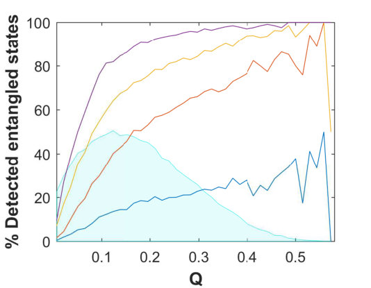 Figure 1
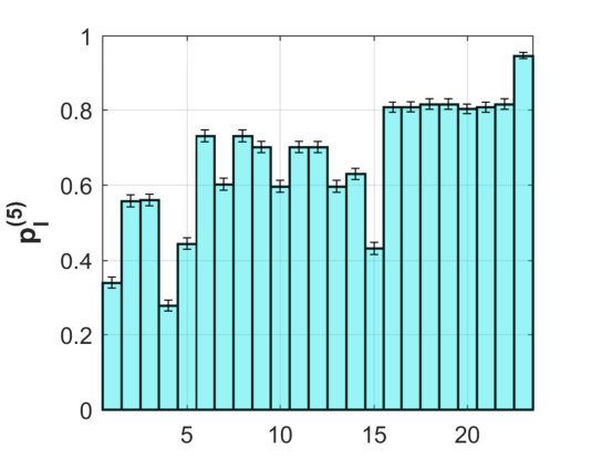 Figure 2
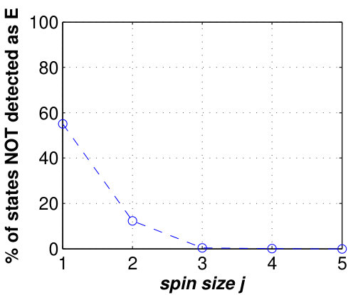 Figure 3
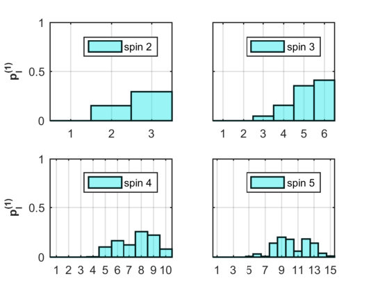 Figure 4
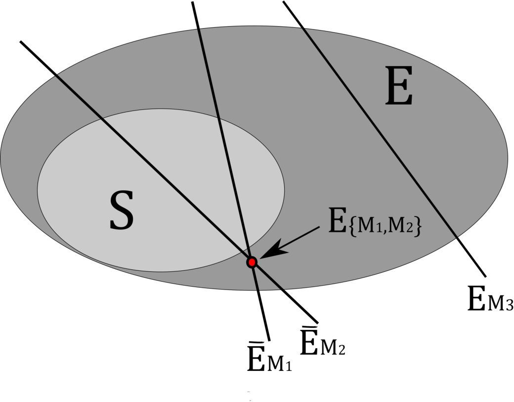 Figure 5
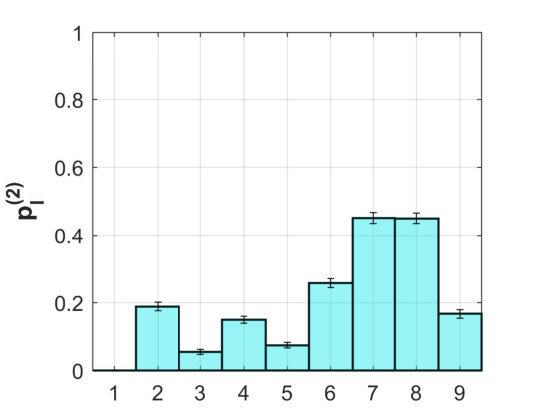 Figure 6
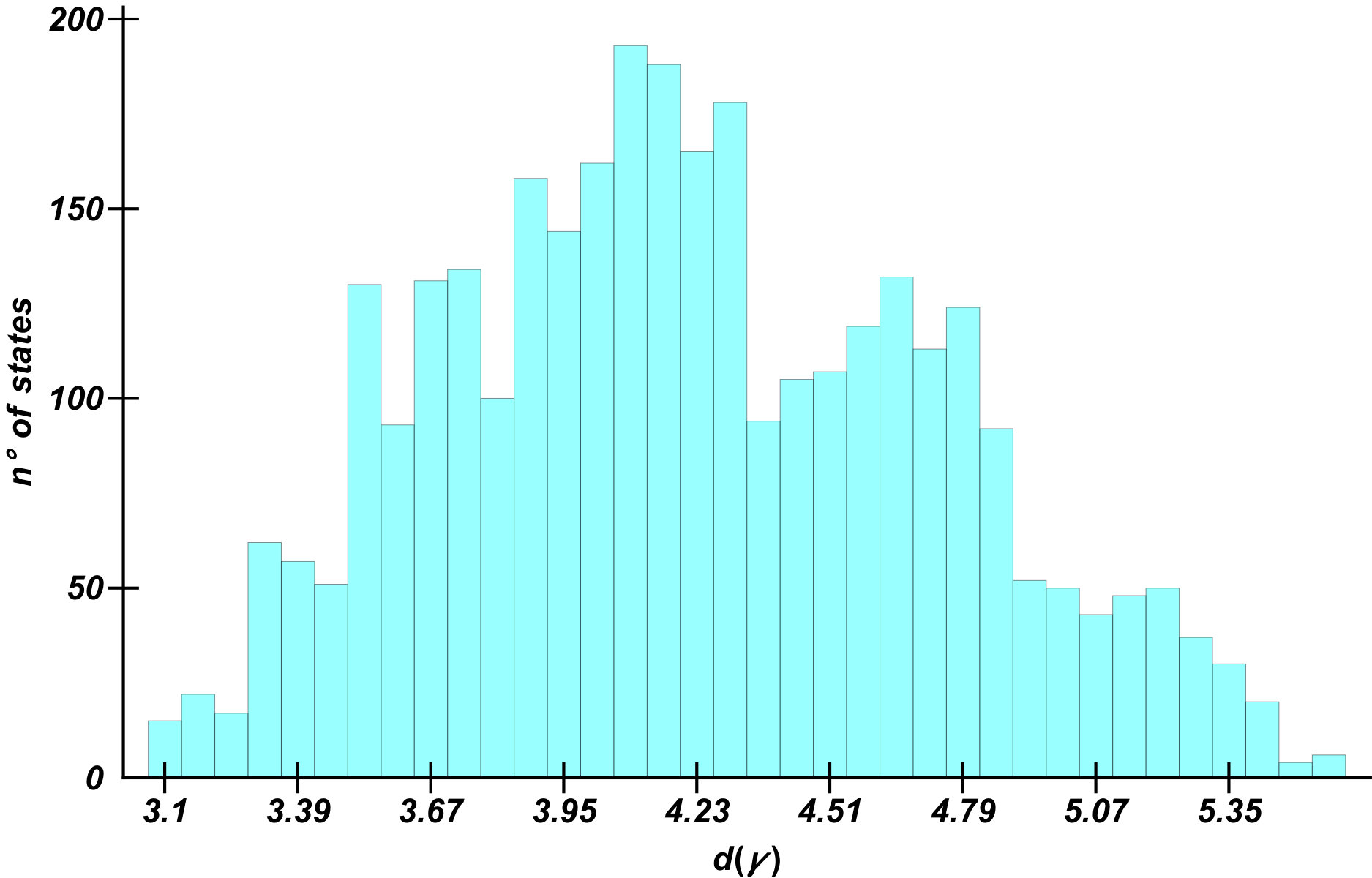 Figure 7
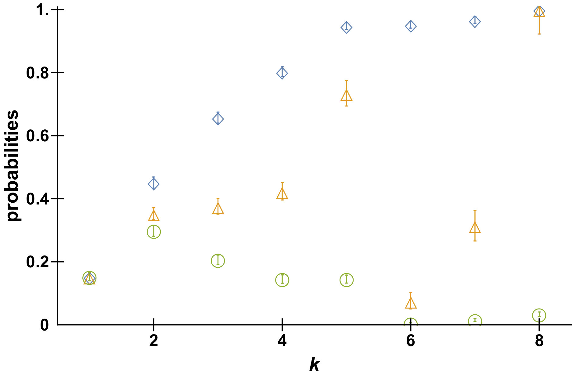 Figure 8
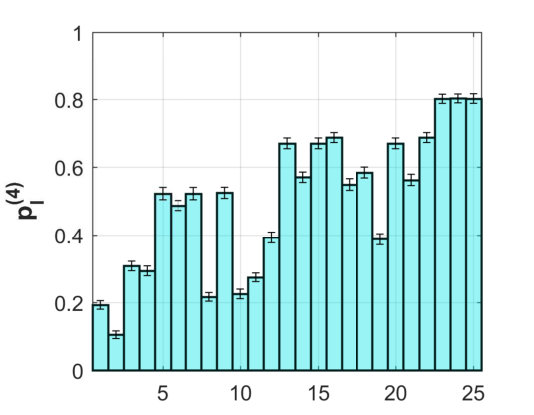 Figure 9
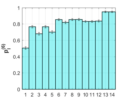 Figure 10
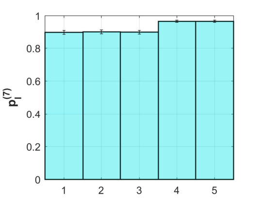 Figure 11
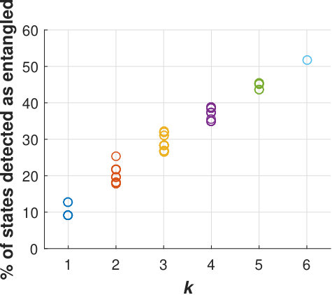 Figure 12
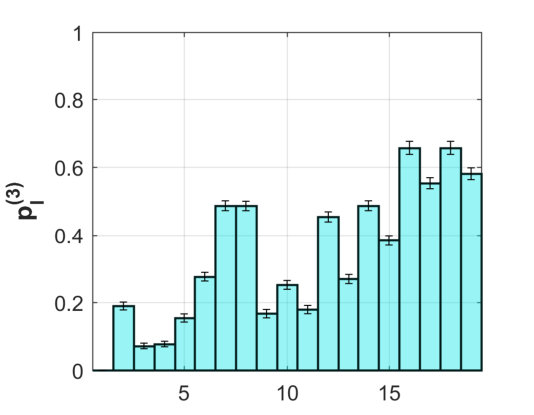 Figure 13
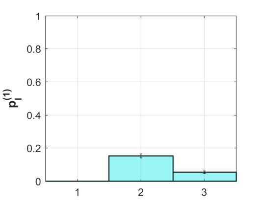 Figure 14
| k | 1 | 2 | 3 | 4 | 5 | 6 | 7 | 8 |
|---|---|---|---|---|---|---|---|---|
| (unordered) | 3 | 9 | 19 | 26 | 23 | 14 | 5 | 1 |
| (ordered; fixed) | 1 | 5 | 26 | 128 | 524 | 1604 | 3228 | 3228 |
| 1 | 2 | 3 | 4 | 5 | 6 | 7 | 8 | 9 | 10 | 11 | 12 | 13 | 14 | 15 | |
| 3 | 10 | 30 | 69 | 132 | 205 | 254 | 254 | 205 | 132 | 69 | 30 | 10 | 3 | 1 |
| 1 | |
|---|---|
| 2 | |
| 3 |
| 1 | |
|---|---|
| 2 | |
| 3 | |
| 4 | |
| 5 | |
| 6 | |
| 7 | |
| 8 | |
| 9 | |
| 10 | |
| 11 | |
| 12 | |
| 13 | |
| 14 | |
| 15 | |
| 16 | |
| 17 | |
| 18 | |
| 19 | |
| 20 | |
| 21 | |
| 22 | |
| 23 | |
| 24 | |
| 25 |
| 1 | |
|---|---|
| 2 | |
| 3 | |
| 4 | |
| 5 | |
| 6 | |
| 7 | |
| 8 | |
| 9 | |
| 10 | |
| 11 | |
| 12 | |
| 13 | |
| 14 | |
| 15 | |
| 16 | |
| 17 | |
| 18 | |
| 19 | |
| 20 | |
| 21 | |
| 22 | |
| 23 |
| 1 | |
|---|---|
| 2 | |
| 3 | |
| 4 | |
| 5 | |
| 6 | |
| 7 | |
| 8 | |
| 9 | |
| 10 | |
| 11 | |
| 12 | |
| 13 | |
| 14 |
| 1 | |
|---|---|
| 2 | |
| 3 | |
| 4 | |
| 5 |
| 1 |
| 1 | |
|---|---|
| 2 | |
| 3 |
| 1 | |
|---|---|
| 2 | |
| 3 | |
| 4 | |
| 5 | |
| 6 | |
| 7 | |
| 8 | |
| 9 | |
| 10 | |
| 11 | |
| 12 | |
| 13 | |
| 14 | |
| 15 |
Peer Reviews
No public reviews on file for this paper yet. If you reviewed it on a platform where reviews are public (OpenReview, ICLR, NeurIPS, ICML), you can paste yours below so the community can read it here.
Videos
No videos yet. Explain this paper in a talk, walkthrough, or lecture? Add one.
Optimal measurement strategies for fast entanglement detection
N. Milazzo
Institut für theoretische Physik, Universität Tübingen, 72076 Tübingen, Germany
LPTMS, CNRS, Univ. Paris-Sud, Université Paris-Saclay, 91405 Orsay, France
D. Braun
Institut für theoretische Physik, Universität Tübingen, 72076 Tübingen, Germany
O. Giraud
LPTMS, CNRS, Univ. Paris-Sud, Université Paris-Saclay, 91405 Orsay, France
(February 13, 2019)
Abstract
With the advance of quantum information technology, the question of how to most efficiently test quantum circuits is becoming of increasing relevance. Here we introduce the statistics of lengths of measurement sequences that allows one to certify entanglement across a given bi-partition of a multi-qubit system over the possible sequence of measurements of random unknown states, and identify the best measurement strategies in the sense of the (on average) shortest measurement sequence of (multi-qubit) Pauli-measurements. The approach is based on the algorithm of truncated moment sequences that allows one to deal naturally with incomplete information, i.e. information that does not fully specify the quantum state. We find that the set of measurements corresponding to diagonal matrix elements of the moment matrix of the state are particularly efficient. For symmetric states their number grows only like the third power of the number of qubits. Their efficiency grows rapidly with , leaving already for less than a fraction of randomly chosen entangled states undetected.
I Introduction
With the availability of the first small quantum processors, the task of characterizing such processors has become a key challenge. Indeed, long before proving full functionality, one of the major questions that faces a quantum processor is whether it “truly” works quantum mechanically — or could rather be explained by classical processes. Similar questions arise already at the level of a quantum state: given a physical system in an unknown quantum state, can the statistics arising from it be explained by a classical state? If the state is fully characterized, one can apply non-classicality measures to find out, but since a mixed quantum state of qubits is specified by real parameters, it is clear that an answer based on full state quantum tomography quickly becomes impractical. In addition, one can only estimate expectation values based on averages over finitely many measurements that are themselves imperfect, and the resulting uncertainty can lead to nonphysical states in the inversion procedure underlying full quantum state tomography. More robust approaches to state tomography are maximum likelihood estimation of the state [1, 2, 3, 4] or Bayesian inference [5, 6], which output estimates of the state that are by construction bona fide physical states, as well as “self-consistent quantum-tomography” not necessarily relying on perfect measurements [7], but none of these approaches remedies the efficiency problem.
Recent developments based on compressed sensing make use of prior information of states. They provide a large gain in efficiency, in particular for the typically low-rank states relevant for quantum information tasks [8, 9, 10, 11, 12], or matrix-product states that describe interacting condensed-matter systems in low dimensions [13, 14]. Machine learning aimed at determining by itself what the best measurements are for a certain task, or to recognize entanglement from measurement data, was considered e.g. in [15, 16, 17, 18], but the efficiency of such approaches needs further study. Other proposals include few-copy multi-particle entanglement detection based on probabilistic verification [19, 20].
For testing quantum circuits, the approach of randomized benchmarking has emerged [21, 22, 23, 24]. Key to this approach is that for estimating fidelities between actual and ideal gate sets, only low moments of the matrix elements are required. In such a case, averaging over the full unitary group can be replaced by averaging over a unitary -design [25], or producing required input states by random quantum circuits (see also [26]). [27, 28] showed that a small number of parameters of a quantum process can be efficiently obtained, but it is not so clear what are the most relevant parameters that should be chosen.
It is often stated that quantum states and quantum processors are much harder to test and characterize than their classical analogues because of the exponential growth of Hilbert space [13, 29, 30]. However, also classically the number of possible memory configurations of bits grows exponentially as — and with of order for a standard laptop computer, it is completely out of the question to test all possible configurations. As costs for integration itself have decayed exponentially according to Moore’s law, for the same reason functional testing of classical memory devices has evolved to the most expensive (since time-consuming) part of the production of integrated memory chips. Functional testing of classical memories has therefore evolved to testing the most critical known configurations with the goal of demonstrating failure of memory cells as quickly as possible. “Most critical” depends on the architecture of the chip, and information on its design goes into the design of memory patterns to be tested. For example, a cell on a given bit-line might resist storing a “0” most likely if all other cells on the same bit line contain a “1”. In MRAM devices, magnetic stray fields from a set of cells can destabilize others in the vicinity when uniformly polarized, etc.
Quantum-information processing may still have a long way to go before such economical pressure on functional testing will be felt. At the moment, rather than showing failure, one would like to prove basic quantum functionalities as quickly as possible. Nevertheless, the principles of classical functional testing can also provide guidance in the current state of affairs in characterizing quantum processors and states: rather than aiming at full quantum tomography, one may want to focus on producing states that are likely to be particularly unstable, and show their “functionality” as quickly as possible. In practice, this will need information about the physical realization of the quantum processor, but in the absence of such input, a reasonable target are highly entangled states, or more generally, highly non-classical states known to be prone to decoherence. Indeed, experimental efforts have concentrated early on on producing such states (see e.g. [31, 32, 33, 34, 35] for states with large numbers of entangled particles).
The question arises then: what is the most efficient measurement strategy to prove that such a state is entangled (or more generally: non-classical)? I.e. what would you choose to measure first, second, and so on, in order to be able to prove as quickly as possible with the limited knowledge about the state that you will gain from those measurements, chosen from a given set, that the state is entangled? What are the minimum and average numbers of measurements needed to prove entanglement, or more generally the statistics of the length of measurement sequences when going down a certain path of measurements?
These are the questions that we start to answer in the present paper. Note that this is not about choosing optimal entanglement witnesses, but rather about deciding whether the intersection of hyperplanes defined by the expectation values of certain observables cuts the set of separable states or not (see Fig. 4). Perfectly suited for answering these questions is the formalism of “truncated moment sequences” (TMS) that we introduced in [36] to the analysis of entanglement. The TMS problem aims at finding a probability measure for which only some moments are known. If the probability measure is furthermore constrained to be supported on a compact set , the problem is known as the -TMS problem. As will be reviewed below, it can be solved with a hierarchy of flat extensions that maps onto a convex optimization algorithm, using a semidefinite relaxation procedure. Each expectation value can be associated with a moment of a measure, and instead of fixing all moments up to a certain order as in the standard TMS algorithm, one might just specify any set of moments. The problem of deciding whether a classical measure that reproduces all these moments exists is then known as the ”-TMS problem” [37]. It can still be solved with a convex optimization algorithm.
In the present work we exploit this approach in order to obtain the statistics of lengths of measurement sequences in the simplest case of two qubits depending on the chosen measurement strategy. For larger numbers of qubits, the full numerical solution of the -TMS problem becomes too demanding, but it turns out that surprisingly efficient sufficient conditions for entanglement can be obtained for symmetric states from the diagonal matrix elements of the moment matrix used in the approach (see below for a definition). These correspond to certain linear combinations of expectation values of (possibly multipartite) measurements in the Pauli basis and have to be positive for a solution of the -TMS problem to exist. Checking the positivity of moment matrices is in fact the first step in the TMS-algorithm, and negativity of any of the diagonal matrix elements hence witnesses entanglement. With these we can find numerical estimates of the fraction of randomly drawn states that are already detected as entangled by just measuring the observables corresponding to the diagonal matrix elements of the moment matrix.
Similar ideas for certifying entanglement with incomplete measurements were already considered in [38] for continuous variable systems. Here we focus on the statistics of lengths of sequences of measurements for multi-qubit systems and the insights that can be drawn from the TMS algorithm which we review in the next section, before applying it to incomplete measurements.
II Framework and notation
We now briefly summarize the TMS algorithm approach described in detail in [36], which will be the framework for the following sections. The basic idea is to map the quantum entanglement problem onto the mathematically well-studied truncated moment problem. Indeed, finding whether an arbitrary multipartite state can be decomposed into product states corresponds to finding about the existence of a probability distribution whose lowest-order moments are fixed. Analytically, the mapping allows one to make use of theorems from the TMS literature providing necessary and sufficient separability conditions; numerically, semidefinite optimization techniques yield an algorithm which gives a certificate of entanglement or separability. The algorithm applies — at least in principle — to arbitrary quantum states with arbitrary number of constituents and arbitrary symmetries between the subparts. The general case is dealt with in [36]; we only recall here the main key points for the case of symmetric states of qubits, defined as mixtures of symmetric pure states (the latter are invariant under any permutation of the qubits). To do so, we will use a convenient representation in terms of symmetric tensors which was introduced in [39], generalizing the Bloch sphere picture of spins. We can write a generic state of a spin- state as
[TABLE]
where is the identity matrix, are the Pauli matrices and is the projector onto the symmetric subspace spanned by the Dicke states (eigenstates of pseudo-angular momentum component and with total angular momentum quantum number ). They can also be seen as symmetric states of spins-1/2 (or qubits). The tensor is then given by
[TABLE]
with . It is real and invariant under permutation of indices, and verifies . Moreover, it has the property that
[TABLE]
for any choice of the . A separable pure state can be seen as a spin-coherent state, which in the representation (2) has tensor entries , with and the unit vector giving the direction of the coherent state on the Bloch sphere. In terms of this tensor representation, a symmetric state is separable if and only if its tensor representation can be written as
[TABLE]
where and is the Bloch vector of the single qubit. If we express (4) in the equivalent integral form
[TABLE]
with , the unit sphere and a positive measure on , we can say that a symmetric state is separable if and only if there exists a positive measure supported by such that all entries of the tensor are given by moments of that measure.
Problems of this type are known as -TMS problems, or -TMS problems in the case of partial knowledge of a state where only a subset of the moments, specified by the set , is known. They can be solved by a semidefinite relaxation procedure. The algorithm proposed in [36] uses indeed semidefinite programming (SDP) and the concept of ”extensions”, already introduced in [40], but based on a matrix of moments and a theorem in the theory of moment sequences. In order to present more clearly the mathematical setting for the -TMS problem, we introduce a more compact notation for Eq. (5). For any -tuple we define a triplet of integers such that , where we use the notation . The degree of the monomial is . We then set . The is a TMS, that is, a sequence of moments of truncated at degree . In case only a subset of these moments is known, we consider the TMS . With this notation we can rewrite (5) as
[TABLE]
To a TMS of degree d, for any integer , we can associate a matrix defined by with , which we call the th order moment matrix. A necessary condition for a TMS to admit a representing measure is that the moment matrix of any order be positive semidefinite. A second necessary condition can be obtained from the polynomial constraint which defines the set . For even degree d we define a ”shifted TMS” of degree , and its moment matrix of order is called the kth-order localizing matrix of . It is necessarily positive semidefinite if a TMS admits a representing measure.
Beyond these two necessary conditions, a sufficient condition was obtained in [41] for even-degree TMS. Namely, if a TMS z of even degree is such that
[TABLE]
then the TMS z admits a representing measure. As the above condition is only sufficient, a TMS admitting a representing measure does not necessarily fulfill it, but one can always search for an extension of it which does. An extension of a TMS y of degree d is defined as any TMS z of degree 2k with , such that for all . An extension z is called flat if it satisfies Eq. (7). If z verifies the sufficient conditions above, then it has a representing measure, and so does y as a restriction of z. Then it is possible to formulate a necessary and sufficient condition for the existence of a representing measure as follows:
Theorem A state is separable if and only if its coordinates are mapped to a TMS such that there exists a flat extension with , and whose corresponding th order moment and localizing matrices are positive semidefinite.
This necessary and sufficient condition can be translated into an algorithm looking for flat extensions of the TMS associated with a quantum state . One runs the algorithm with input the state (that means fixing for all ), starting from the lowest possible extension order . If the corresponding SDP is ”infeasible”, then the conditions of the theorem are not satisfied and the TMS admits no representing measure , which means that the quantum state whose coordinates are given by is entangled. If, on the contrary, the SDP problem is ”feasible”, then the TMS admits a representing measure, and the corresponding quantum state is separable. The algorithm also extends to the case of non-symmetric states (see [36] for further detail).
III Unordered measurements
III.1 Goal
Let us now consider the question raised in the introduction. Our goal is to identify the smallest set of measurements that should be performed on an unknown spin state to detect that it is entangled. This is possible in a real experiment when many identical copies of the same state are available, so that a different measurement can be performed on each copy. We will first discuss the case of symmetric two-qubit states, which, as we will see in detail, already presents some complexity. In this case the PPT criterion [42, 43] applied to a partially known density matrix would also provide a way of detecting entanglement via SDP. Nevertheless, we will use our TMS approach, since it allows for a straightforward generalization to arbitrary number of qubits and moreover it applies SDP to the matrix of moments, whose entries are directly given by measurement results.
III.2 Symmetries and measurements
For a symmetric two-qubit state , Eq. (2) with gives
[TABLE]
with and . In this case the tensor reduces to a real symmetric matrix. Its 10 entries with can be seen as the result of the measurement of the joint operator . We now ask which are the possible measurements that we can perform and how many there are; the observables considered are the most simple, i.e. Pauli spin operators. Let us denote these inequivalent measurement operators as
[TABLE]
(we omit the identity operator corresponding to , and we always order sets of measurements in degree-lexicographic order). For instance, is the measurement of on the first qubit and of on the second one (or the reverse), while is the measurement of the joint operator . Since the tensor is such that
[TABLE]
only two of the three diagonal entries are independent, and measuring two out of three of the observables , and yields the third value. Thus, carrying a tomography to its end for a single spin-1 state consists in measuring 8 observables in total.
Our aim is to find the probability that a state is detected as entangled if only the result of measurements of a certain subset of these 8 observables is known. Let us first of all observe that these probabilities should not depend on the choice of the reference frame for the axes along which the measurement is performed. As a consequence, the results for equivalent measurements in different directions should be the same. We will therefore only consider sets which are non-equivalent under permutation of the axes, that is, sets that are unchanged under transpositions , which exchange two axes, and cyclic permutations and .
We will consider all possible non-equivalent sets of measurements, with , disregarding the order of measurements within a set. For sets of length we can easily see that the non-equivalent measurements are only three: . Indeed, the local measurements are equivalent, as well as the two-qubit ”diagonal” measurements (giving the diagonal entries of matrix ), and also the two-qubit ”off-diagonal” measurements (giving its off-diagonal entries). For , there are possible pairs, among which only 9 are inequivalent, namely . We denote by the number of non-equivalent sets of measurements, and we report it in Table 1. The corresponding complete lists of measurements for all is given in Appendix A.
For each , our question reduces to finding out which set of measurements, among the possible ones, yields the highest entanglement detection probability. Note that performing measurements is not exactly equivalent to having fixed moments. Indeed, since moments are related by Eq. (10), measuring and fixes the three moments and . Any measurement set of length containing both and will in fact correspond to a TMS with moments fixed. We therefore always discard from the measurement sets.
III.3 Set probabilities
In terms of the TMS algorithm, performing a measurement means obtaining a value of a tensor entry , or equivalently of a moment . Performing measurements means that the moments corresponding to those measurements are fixed, as well as all moments obtained via relation (3).
For a given number of measurements, we indicate a specific set of measurements among the possible ones as . For instance, if , we could have which corresponds to the set of measurements .
If we consider a fixed and a fixed subset of the set of observables , we denote the sample space of outcomes of the -TMS algorithm applied to the moments of an entangled state as . It contains two possible outcomes, to which a probability can be assigned: detecting the state as entangled (if the associated SDP is infeasible, i.e. if the state is entangled), with probability , or not detecting it as entangled (if the SDP is feasible, i.e. if the state with such moments fixed is still compatible with a separable state), with probability . To shorten notation we may denote as , which entails .
These probabilities can be estimated by running the TMS algorithm for each and each , testing all the possible sets of measurements. Note that always increases, in the sense that for . Indeed, the probability not to detect entanglement with more and more measurements goes down with the number of measurements. In other words, fixing more moments reduces the probability of finding a measure with such moments. Once all eight measurements are done the state is fixed uniquely, so that for entangled states . To estimate the values for the probabilities , we sample states from the set of symmetric two-qubit states. We generated random states drawn from the Hilbert-Schmidt ensemble of matrices , with a complex matrix with independent Gaussian entries (following [44]). Among them were 1843 separable states that we discarded, implying the normalization condition for full tomography. For each measurement set and each entangled state in our sample the TMS algorithm was run with the corresponding moments fixed; the results for the probabilities are reported in Figs. 1 and 2.
Some probabilities appear to be equal. This is for instance the case of probabilities labeled 16 and 18 for . This is a consequence of an additional symmetry due to the linear equations that measurement results must satisfy. In the case , labels 16 and 18 correspond to and respectively. Since, as we already mentioned, knowing the result of any two diagonal measurements gives the third one because of Eq. (10), the information acquired by measuring the observables corresponding to labels 16 and 18 is equivalent, and therefore the probabilities must be equal.
The optimal choice of measurements at fixed corresponds to the sets giving the highest probability of detecting entanglement. For the highest value of corresponds to the measurement #2, . For it corresponds to #7, . For the highest values correspond to two measurements: #16, , and #18, . For it corresponds to #23, , #24, , and #25, . Again, the degeneracy of the optimal set reflects the equivalence of the corresponding sets once (10) is taken into account. For , the sets in fact correspond to cases where measuring two observables fixes three moments.
III.4 Quantumness
For a fixed set of measurements one can ask whether the rate of detected entangled states depends on how quantum a state is. For an arbitrary state , quantumness may be defined in several different ways; we follow here the definition given in [45], based on spin-coherent states. These are a generalization of the usual coherent states of the harmonic oscillator used in quantum optics to spins; they correspond to spin states which minimize a particular uncertainty relation, and they move as classical phase space points under a Hamiltonian linear in the angular momentum operators [46, 47]. As any spin-1/2 pure state has this property, an arbitrary -qubit spin-coherent state can be defined as with a one-qubit state.
Quantumness is then defined as the Hilbert-Schmidt distance to the convex set of classical spin states [48], that is the ensemble of all density matrices which can be expressed as a mixture of spin-coherent states with positive weights (or in other words the set is the convex hull of spin-coherent states). Namely, the quantumness is given by
[TABLE]
where is the Hilbert-Schmidt norm. For all the property holds, with equality for classical states . Results are reported in Fig. 3, up to for the optimal sets of measurements given above. We can observe that the rate of detected entangled states increases with the quantumness of the states, or in other words, the more quantum a state is the faster it is detected as entangled.
IV Ordered measurements
IV.1 The setting
In the previous section we assumed that observables are measured among the 8 possible ones and that the TMS algorithm is subsequently run. Of course, we can imagine a different experimental protocol where we would perform a measurement, run the TMS algorithm with a single moment fixed, and then, only in the case where the state is not detected as entangled, perform a second measurement and run the TMS algorithm again with two moments fixed, and so on until entanglement is detected or full tomography is achieved. In this setting, we need to distinguish the different ordered arrangements of each -element subset of .
In the following, we call an ordered sequence of measurements a path, and we denote it by . To distinguish it from a set, we denote it as a tuple with round parentheses, such as . A path of length can be alternatively seen as a list of sets of increasing size given by the restriction of the path to the first observables with . For instance for the path can be seen as the list , , and (as usual we write sets in lexicographical order since the order within a set does not matter).
Considering all paths of length 8 would require an exceedingly long computational time. For this reason, we slightly simplify the problem by fixing the first measurement to perform. The most reasonable choice, looking at the results in Fig. 1, is to fix it as a diagonal observable , or , since for it detects the largest fraction of entangled states. Up to relabelling of the axes, we can take as first element, since, as before, we only keep non-equivalent paths. To find these paths, we define a canonical representation of a path of length by considering its equivalent list of sets of length . For each of these sets we choose the first one in lexicographical order among the ones that are obtained by relabelling of the axes. The list of sets obtained in this way is the canonical representation of . Two paths are equivalent if they have the same canonical representation. We report the number of non-equivalent paths of length in Table 1, where e.g. for the non-equivalent sequences will be ,, , , and .
IV.2 Path probabilities
We now show how to retrieve the results for this more general case from the obtained in the previous section. The probability to detect the state as entangled after the first measurement, say , is , given by the previous section. The probability to detect the state as entangled after the second measurement, say , is then , which is the probability of detecting entanglement with the second measurement given that it was not detected with the first one. This quantity now depends on which measurement is performed first. This is illustrated in Fig. 4.
Using the theorem of total probability, we have
[TABLE]
Since and we get
[TABLE]
Thus, the conditional probability we are looking for can be expressed solely in terms of the of the previous section.
Let then be a path of length . We define
[TABLE]
as the probability of detecting entanglement at step k in given that no entanglement was detected up to the step . By a reasoning similar to the one leading to Eq. (13), we can express in terms of the , as
[TABLE]
In particular, since (as nothing is measured, and hence detected as entangled, at level 0), we have . Inverting (15) one obtains in terms of as .
A third natural probability to consider is related to our measurement algorithm, where we perform TMS calculations at step only if the state was compatible with a separable state. We define as the probability of stopping exactly at the th level when measurements are taken along path . It can be written as the joint probability . Using the identity , can be expressed as . It can be rewritten in terms of or as
[TABLE]
IV.3 Best path
Using (15)–(16) and the numerical results of the previous section, we can obtain a numerical estimate of the and the for all possible paths. The optimal path is the one that detects as quickly as possible (on average) if the state is entangled. To identify among all possible ones we define the average depth at which our algorithm stops as
[TABLE]
Expressing Eq. (17) in words, gives the number of measurements that one needs to perform, on average, to detect a state as entangled, following the path . Each path will be characterized by this number and in particular the shortest path will be given by
[TABLE]
The distribution of over all 3228 paths of length eight for symmetric states of two qubits is reported in Fig. 5.
The minimum value found for is , while the maximum value is . The minimum value is degenerate and corresponds to three optimal paths. Although these three paths do not have the same canonical representation they lead to the same value because of condition (10). If one considered that knowing two diagonal moments is equivalent to knowing them all, and included in the symmetrization the third diagonal moment once the first two are measured, there would be a unique optimal path. We report here one of the three equivalent optimal paths: ; choosing this path, one only needs to perform (in average) three measurements to detect a state as entangled. These three measurements give access to the two diagonal moments (and thus all of them via (10)), and one of the off-diagonal ones. The probabilities relative to this best path are shown in Fig. 6.
Rewriting in terms of we get
[TABLE]
It turns out that choosing measurements according to coincides (within the error bars) with choosing for each , , the best set of measurements, i.e. the one with the highest probability of detecting entanglement at a given level (highest among the possibilities for each k). This is not obvious, and it is not always the case: a counter-example is given by a binary tree of depth 4 in which the random probabilities satisfy the same constraint as in our case, i.e. and the four paths have probabilities: . It is easily verified that the best path, with , is the second one, which at depth does not have the highest , so the minimal does not always correspond to the path with the highest at each step.
In practice, joint measurements such as might be more challenging to implement than two single measurements , as qubits need a unitary operation to entangle them first and then two local measurements. In such a case, one might modify (17) with another factor for each path that takes such additional costs into account. Also, we base our analysis on average values of measurement outcomes which we took as known with arbitrary precision. This is, of course, an idealization. In practice, only a finite number of measurements can be performed, leading to statistical error bars for each moment. These can in principle be taken into account in the TMS algorithm, but increase computational time. Both of these points are beyond the scope of the present paper.
V Non-symmetric case
So far we restricted ourselves to symmetric states of two qubits. Let us now consider the generic case of arbitrary two-qubit non-symmetric states. In this case we can still exploit the TMS algorithm, with the following differences [36]. The bipartite state acts on the tensor product of Hilbert spaces and each of them has now its own set of variables and ; we will label these variables as (), with . The compact set K is now the product of two Bloch spheres. The set of possible measurements is
[TABLE]
For example, is the measurement of and is the measurement of the joint operator . Up to relabelling the variables for each qubit, some sets of measurement operators are equivalent. The number of non-equivalent sets of measurements is obtained by applying the 36 possible permutations on the (). This number is reported in Table 2 for .
The number increases fast with , and so does the size of the moment matrices considered in the TMS algorithm: indeed, because of condition (7), the algorithm always searches at least for the first extension; in both cases (symmetric and non-symmetric) the smallest extension corresponds to the moment matrix of order . In the symmetric case it is a matrix, while in the non symmetric case it already becomes a matrix which contains all the monomials up to degree 4 for the set of variables , with , i.e. moments versus in the symmetric case. For the previous reasons computational times become an issue in the non-symmetric case. Nevertheless we could estimate probabilities up to , running the TMS algorithm over a database of 50000 non-symmetric two-qubit random states. What we observe is that no state is detected as entangled with only one measurement, a tiny fraction ( ) is detected as entangled by the combination of two measurements , and the biggest fraction of states detected as entangled for are given respectively by the set of measurements (), (), (). This is a big difference compared to the symmetric case, in which we could detect of the states as entangled with a single measurement, already with two measurements and almost all states with five measurements.
VI Higher spin-j
Going back to the case of symmetric states, we can also get an idea of how complexity changes for higher spin sizes; indeed, the size of the set in the symmetric case corresponds to the sum of the number of monomials in three variables up to degree , where is the spin size. These numbers form the sequence of triangular numbers ; we can then write that for any spin- is
[TABLE]
where we subtract since the first element of is always the identity. However, in this case, we can still have some information looking at the expression for the tensor representation of a separable state in (4). Indeed, for an even number of qubits (integer spins) we can look at the diagonal tensor entries, which are defined as the entries of the form with . These correspond to terms of the form ; it follows that for a separable state these entries are positive, since the are real and . Therefore measuring a negative value for any of the corresponding measurement operators means detecting entanglement; we indicate the operators corresponding to the diagonal entries of the tensor with . We can then restrict our investigation for an integer spin to these observables, which are further reduced by symmetry to . We report in Fig. 7 the number of entangled states that are not detected by any of the observables for spin size (for each we used a sample of random states from which we again removed the separable ones). The number of not detected entangled states decreases with the spin size and already for all the states in the sample are detected; we can also observe that restricting the analysis to these observables already gives significant information for spin- and spin- and almost complete information for spin-.
Moreover, we can also compare these observables to see which is the most efficient measurement to perform as we did for the spin- case; to estimate the corresponding , we will again only consider sets which are non-equivalent under permutation of the axes, performing the transformations described in section III.2. The results are shown in Fig. 8.
The question arises whether similarly efficient measurements can be found for half-integer spin . It was recently shown in [49] how the positive-partial-transpose (PPT) separability criterion for symmetric states of multi-qubit systems can be formulated in terms of matrix inequalities based on the tensor representation in Eq. (2). It is possible to construct a matrix from the tensor representation of the state and show that it is similar to the partial transpose of the density matrix written in the computational basis. In the case of spin- this matrix is a Hermitian matrix given by , where are the Pauli-matrix components, and its positivity is a necessary and sufficient classicality criterion; as a consequence, the positivity of the diagonal entries is a necessary condition for a separable state. We can again restrict our investigation to the corresponding observables , but this time it implies the measurement of sets of two observables. Indeed, in terms of the tensor entries , the diagonal entries of are , so we need to compare pairs of outcomes. Recalling that , we can neglect the first entry, since the condition is always satisfied. The results of such investigation for the other six pairs and for their combinations (all the sets, with ) are reported in Fig. 9. As before, we can gain already relevant information from this restricted analysis.
VII Conclusions
In summary, we have studied the statistics of lengths of measurement sequences for multi-qubit systems that allow one to detect entanglement without any prior information about the state, both for unordered sets of measurements and ordered ones (i.e. measurement paths). For symmetric states of two qubits, we have identified the best measurement path that results, on average over all randomly chosen entangled states, in a proof of entanglement with 3.07 measurements (compared to 8 measurements needed for full tomography in this case). For larger numbers of qubits in symmetric states, we found that measurements based on the diagonal matrix elements of the moment matrix of the state become very efficient in detecting entanglement. Their number grows like , and already for qubits the number of states not detected as entangled has decayed to about or smaller. For non-symmetric states, substantially larger numbers of measurements are needed to detect entanglement with certainty: at least two measurements are needed for two-qubit states, resulting in only about 1% detection probability, however. With five measurements the probability increases to about 23%. The work is based on the truncated moment sequence algorithm that naturally allows one to deal with missing data. It is very flexible and can be easily adapted to experimentally relevant ensembles of states and other side-conditions, such as sets of measurements that can be implemented, or more elaborate cost functions.
Acknowledgments
DB thanks OG, the LPTMS, and the Université Paris-Saclay for hospitality.
Appendix A Unordered measurement sets
We list here all the unique sets of measurements for .
Appendix B Non-equivalent diagonal observables
We list here all the non-equivalent observables for spin-, .
The reference list from the paper itself. Each links out to its DOI / PubMed record.
- 1James et al. [2001] D. F. V. James, P. G. Kwiat, W. J. Munro, and A. G. White, Phys. Rev. A 64 , 052312 (2001).
- 2Blume-Kohout [2010 a] R. Blume-Kohout, Physical Review Letters 105 (2010 a).
- 3Hradil [1997] Z. Hradil, Phys. Rev. A 55 , R 1561 (1997).
- 4Baumgratz et al. [2013] T. Baumgratz, A. Nüßeler, M. Cramer, and M. B. Plenio, New J. Phys. 15 , 125004 (2013).
- 5Blume-Kohout [2010 b] R. Blume-Kohout, New J. Phys. 12 , 043034 (2010 b).
- 6Rau [2010] J. Rau, Phys. Rev. A 82 , 012104 (2010).
- 7Merkel et al. [2013] S. T. Merkel, J. M. Gambetta, J. A. Smolin, S. Poletto, A. D. Córcoles, B. R. Johnson, C. A. Ryan, and M. Steffen, Phys. Rev. A 87 , 062119 (2013).
- 8Gross et al. [2010] D. Gross, Y.-K. Liu, S. T. Flammia, S. Becker, and J. Eisert, Phys. Rev. Lett. 105 , 150401 (2010).