Analysis of the Block Coordinate Descent Method for Linear Ill-Posed Problems
Simon Rabanser, Lukas Neumann, Markus Haltmeier

TL;DR
This paper analyzes the convergence of block coordinate descent (BCD) methods for linear inverse problems, demonstrating that under certain conditions, BCD with proper stopping criteria acts as a regularization method, supported by numerical experiments.
Contribution
The paper provides the first convergence analysis of BCD for inverse problems and shows it can serve as a regularization method under specific tensor product operator conditions.
Findings
BCD with stopping criteria converges for tensor product operators
Numerical experiments compare BCD and full gradient descent
Tests include linear and non-linear inverse problems
Abstract
Block coordinate descent (BCD) methods approach optimization problems by performing gradient steps along alternating subgroups of coordinates. This is in contrast to full gradient descent, where a gradient step updates all coordinates simultaneously. BCD has been demonstrated to accelerate the gradient method in many practical large-scale applications. Despite its success no convergence analysis for inverse problems is known so far. In this paper, we investigate the BCD method for solving linear inverse problems. As main theoretical result, we show that for operators having a particular tensor product form, the BCD method combined with an appropriate stopping criterion yields a convergent regularization method. To illustrate the theory, we perform numerical experiments comparing the BCD and the full gradient descent method for a system of integral equations. We also present numerical…
Click any figure to enlarge with its caption.
 Figure 1
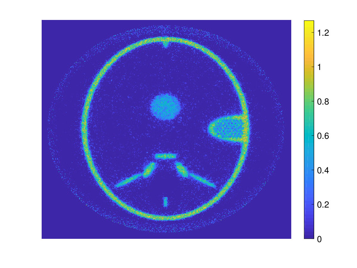 Figure 2
 Figure 3
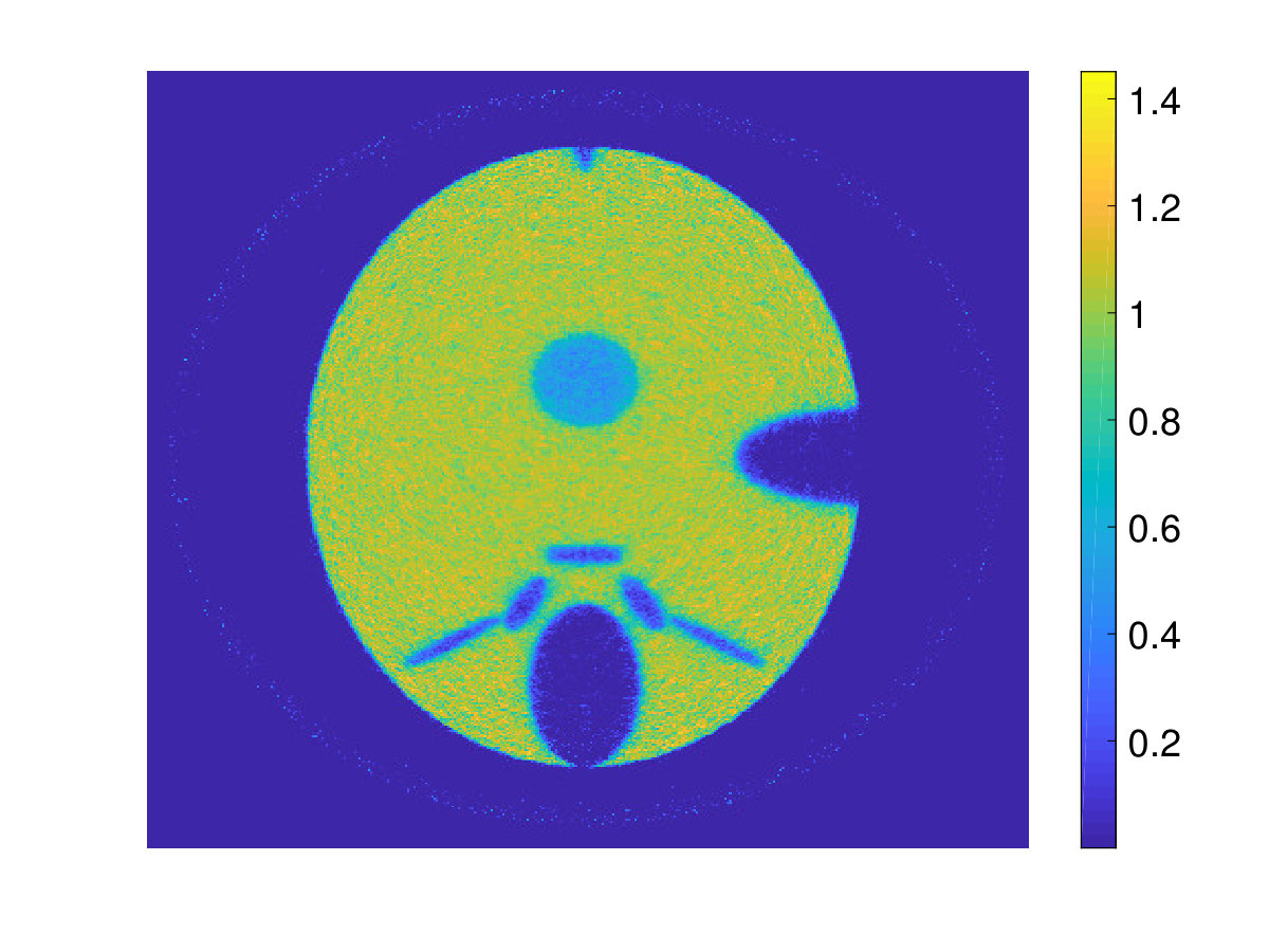 Figure 4
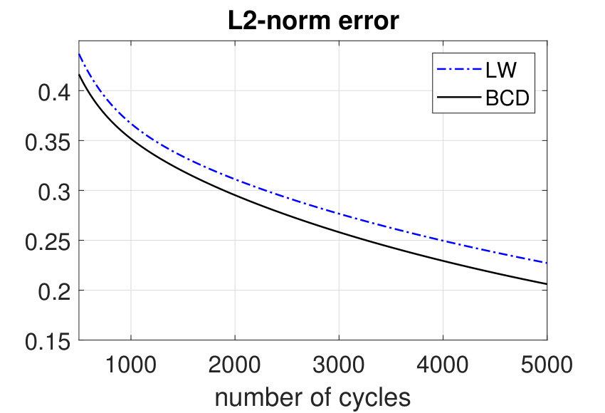 Figure 5
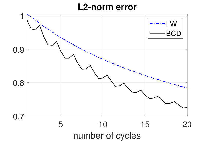 Figure 6
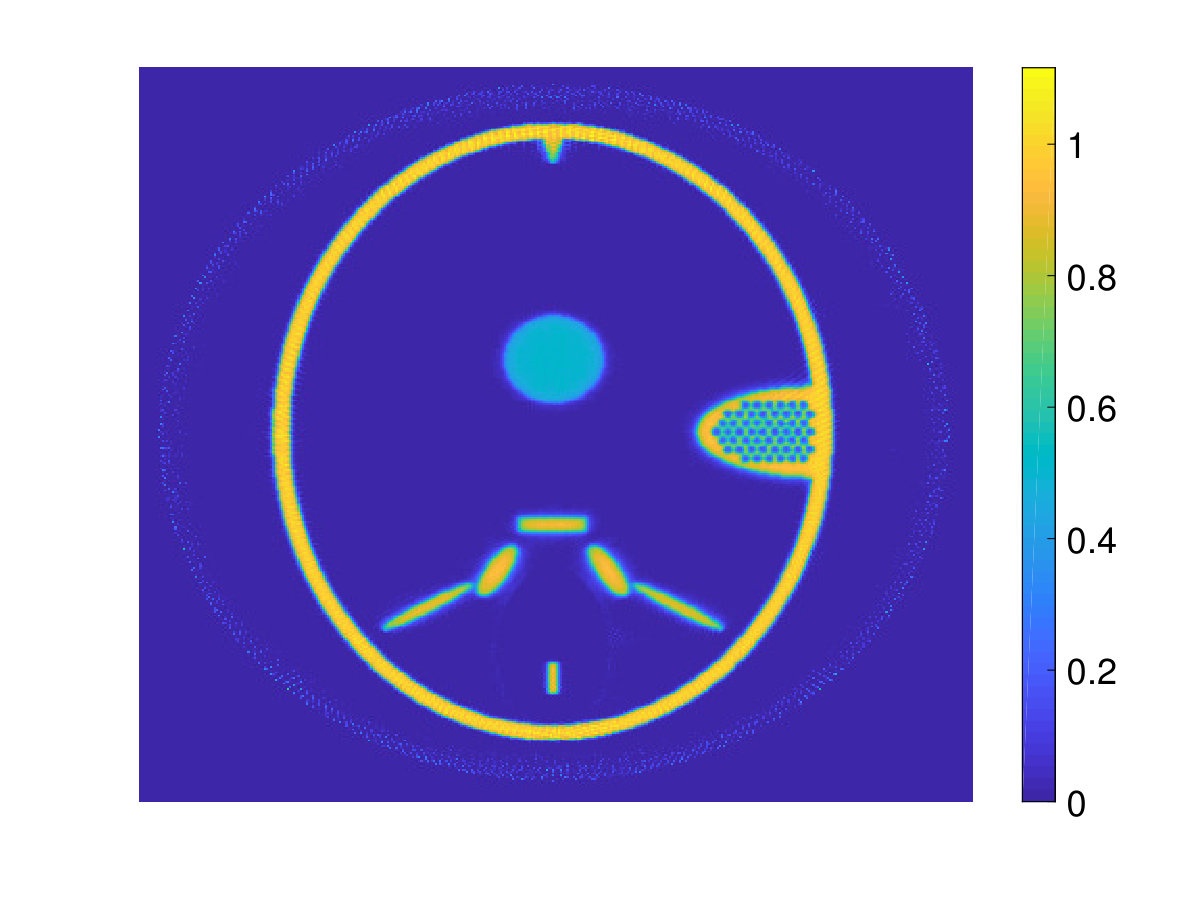 Figure 7
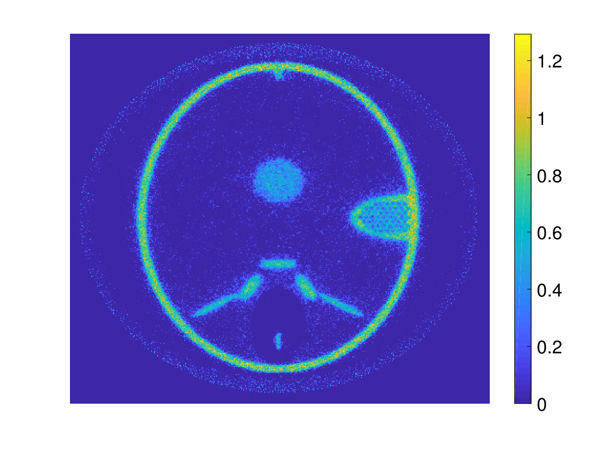 Figure 8
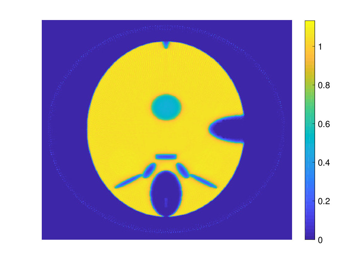 Figure 9
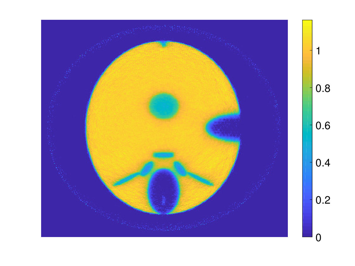 Figure 10
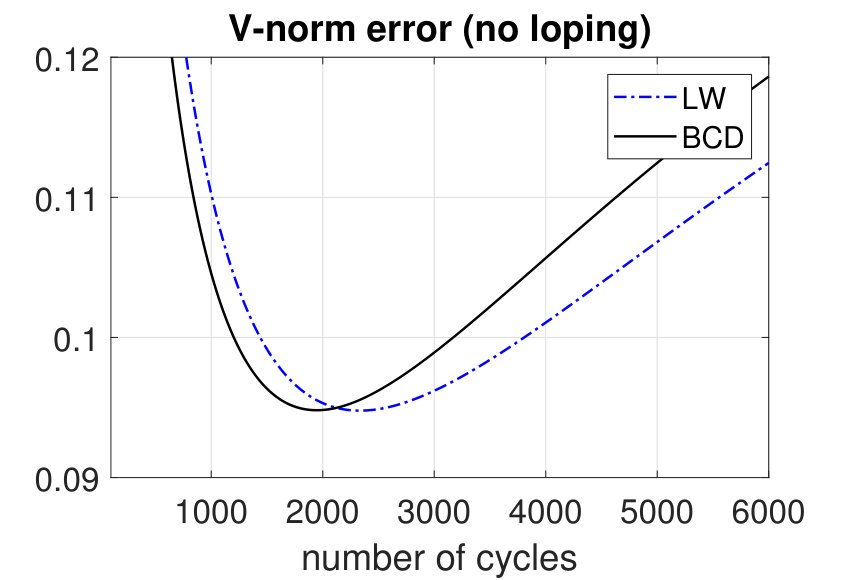 Figure 11
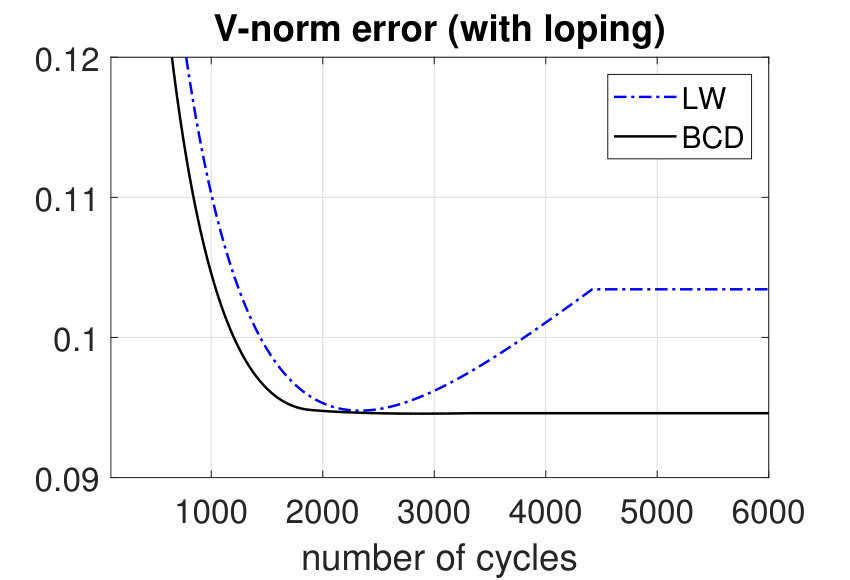 Figure 12
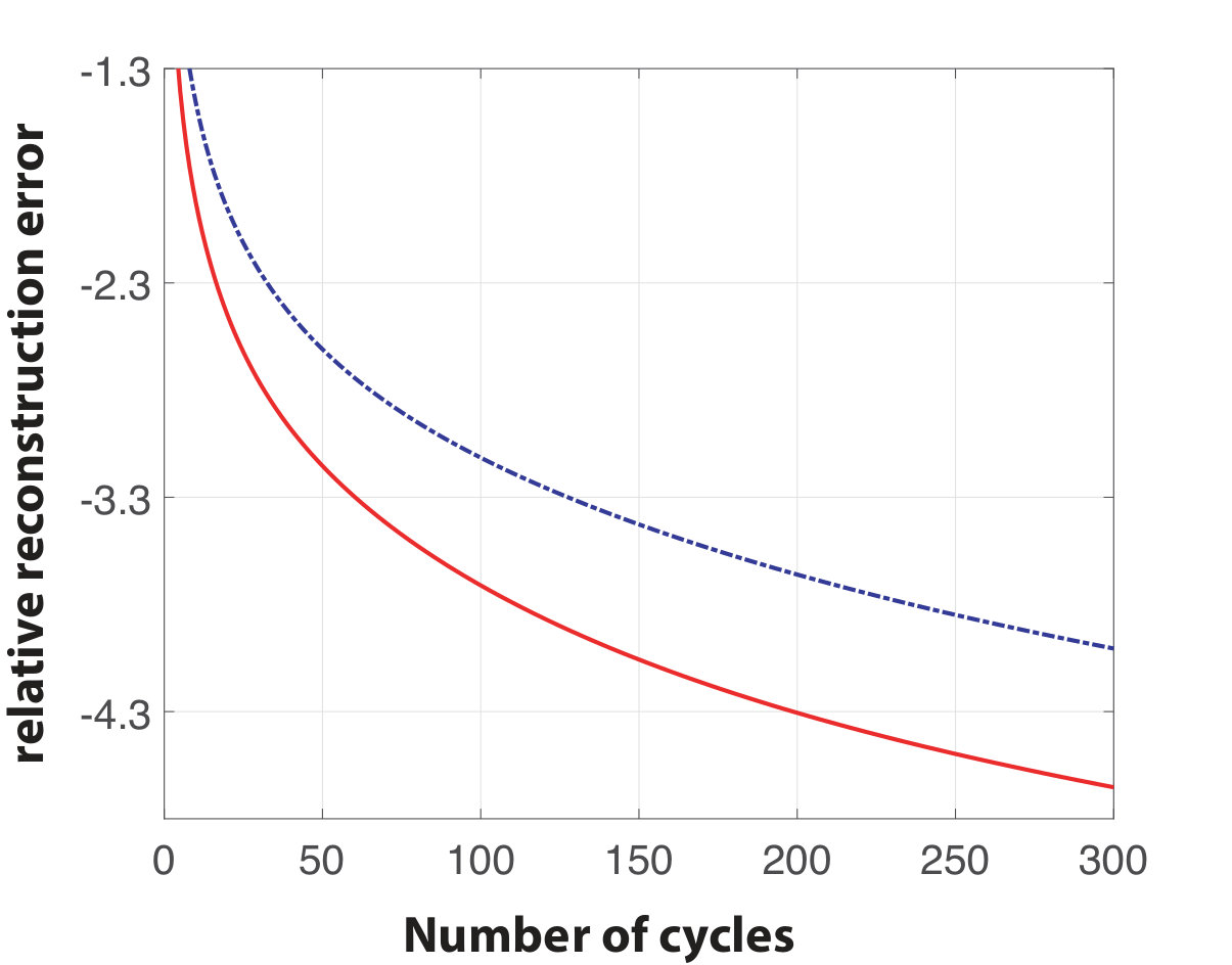 Figure 13
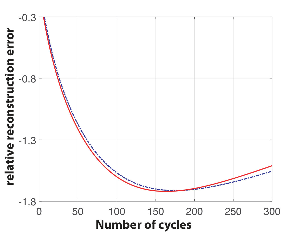 Figure 14
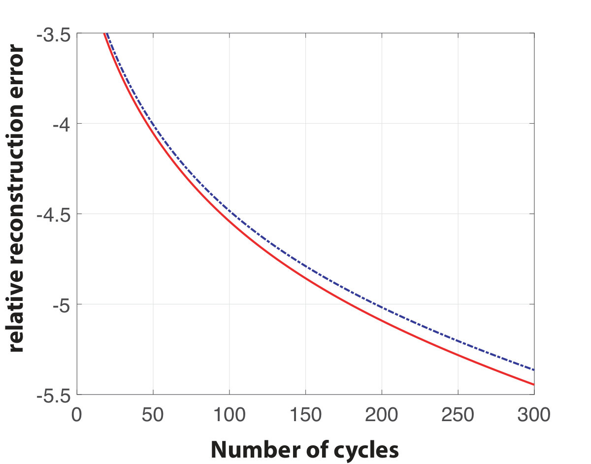 Figure 15
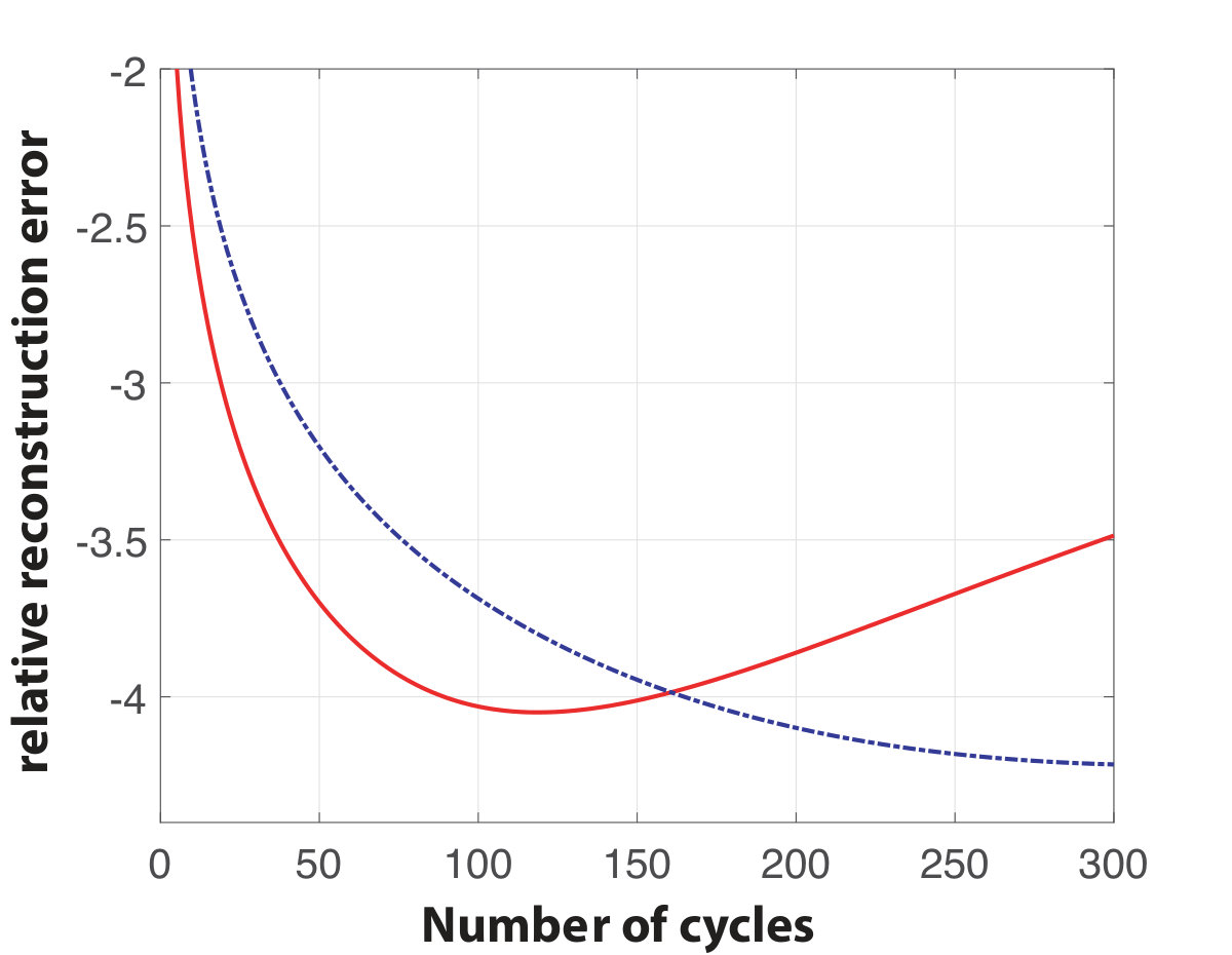 Figure 16
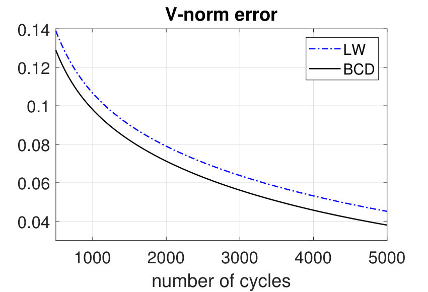 Figure 17
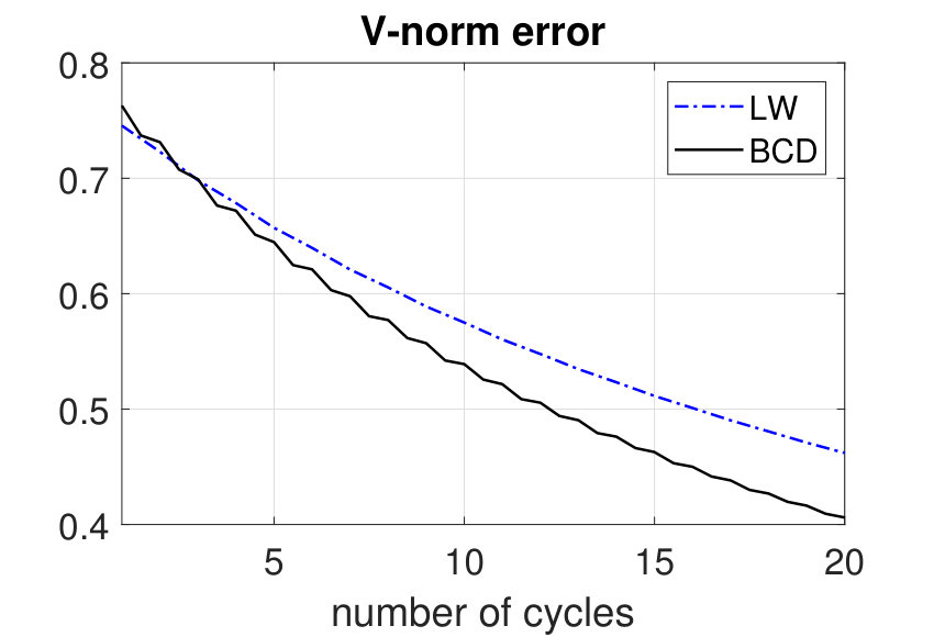 Figure 18
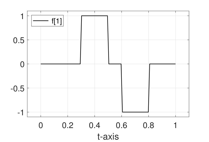 Figure 19
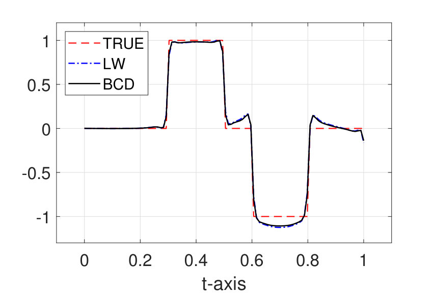 Figure 20
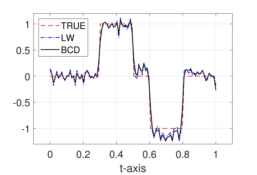 Figure 21
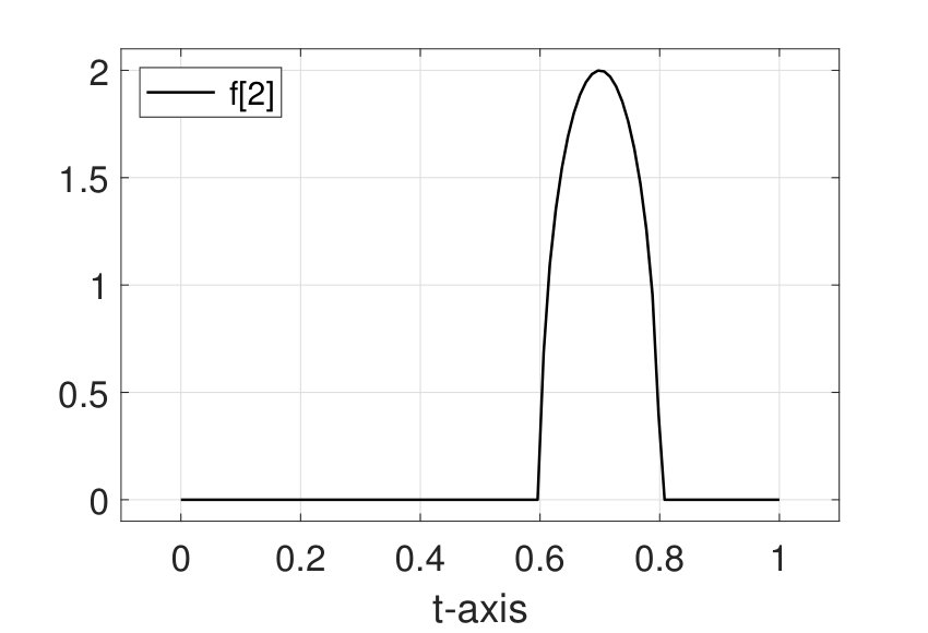 Figure 22
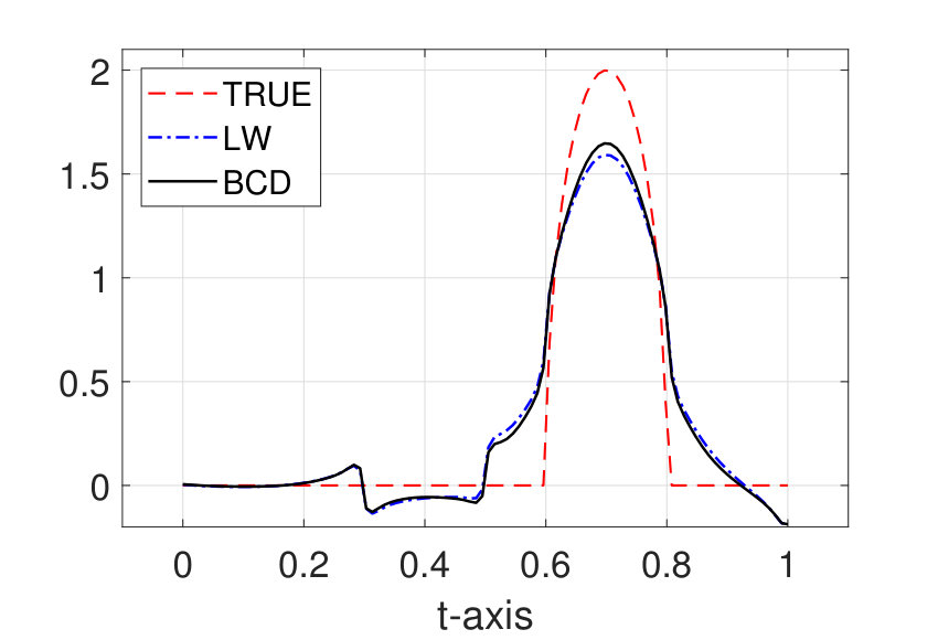 Figure 23
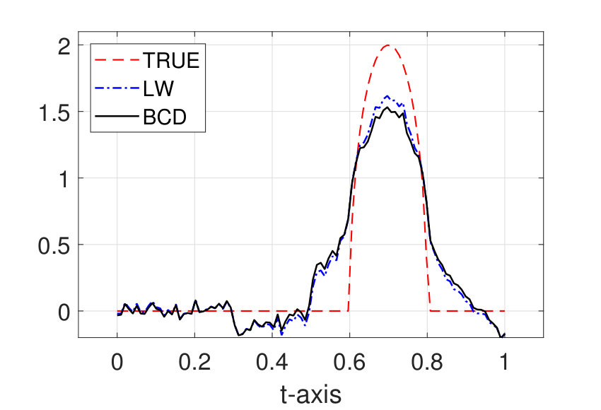 Figure 24
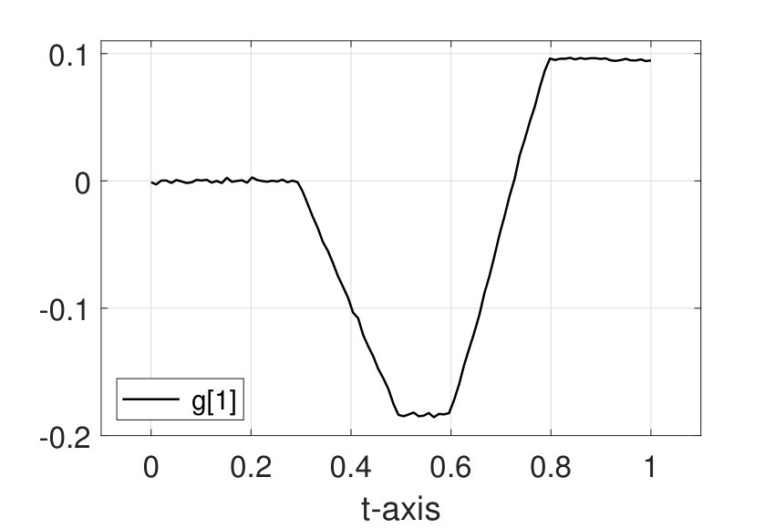 Figure 25
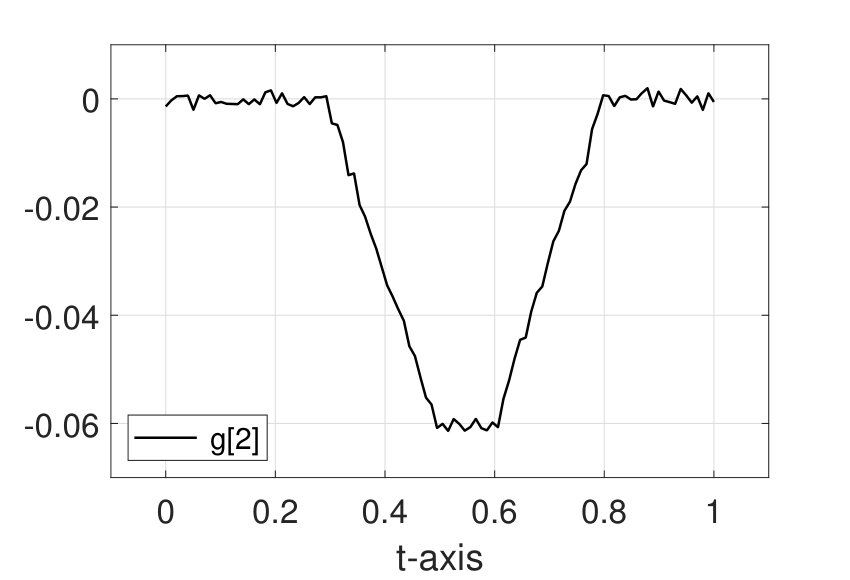 Figure 26
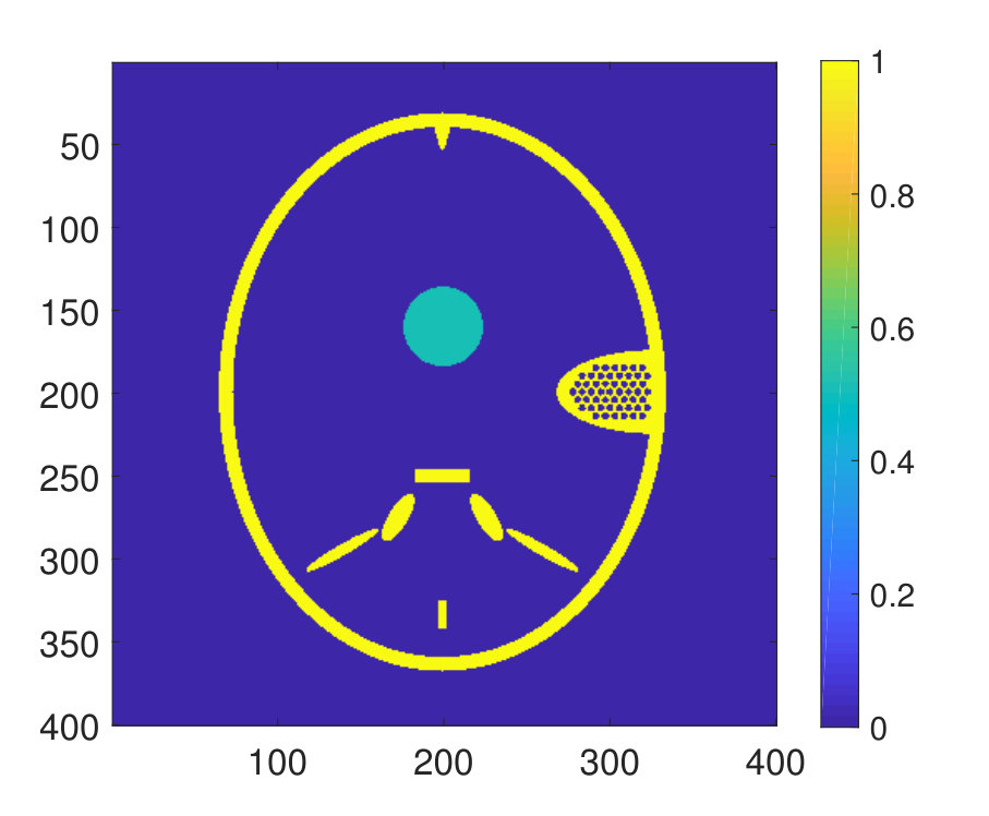 Figure 27
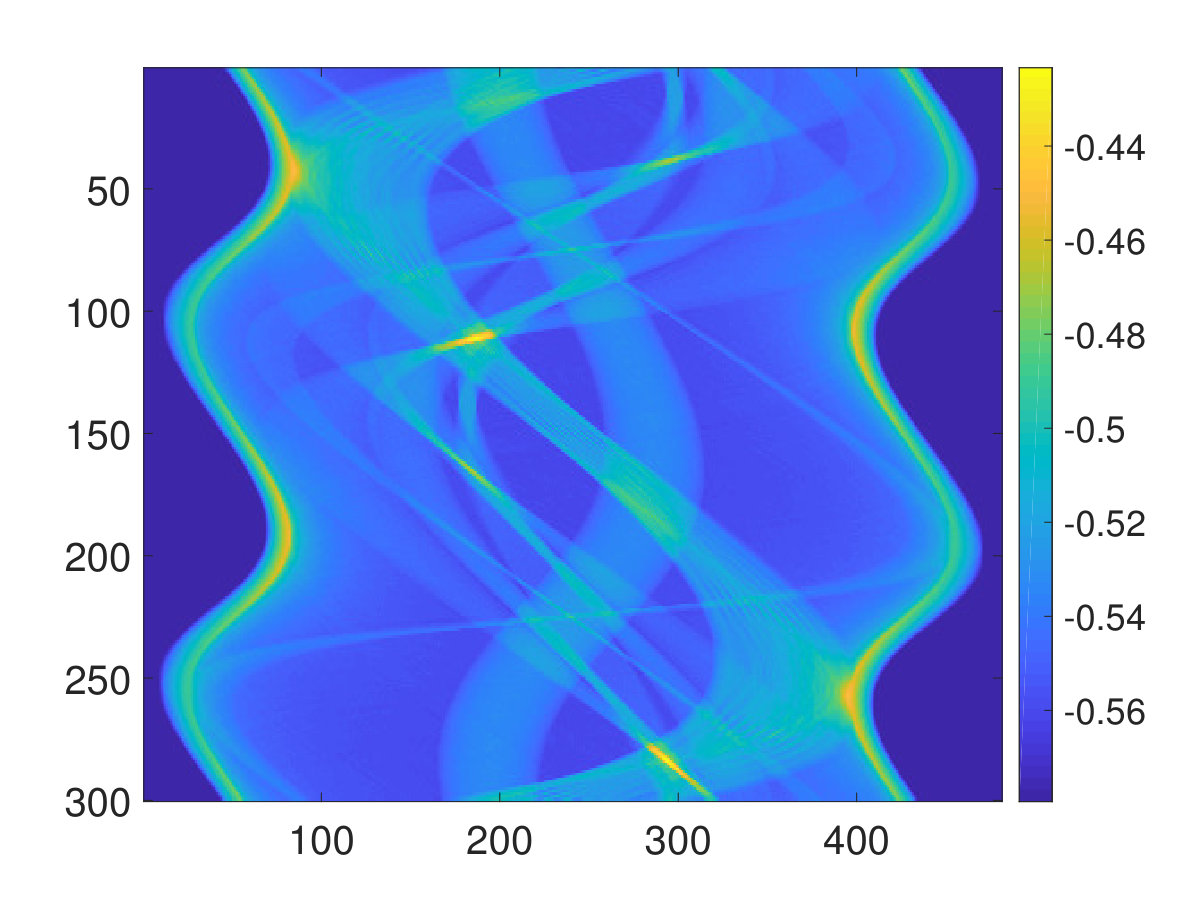 Figure 28
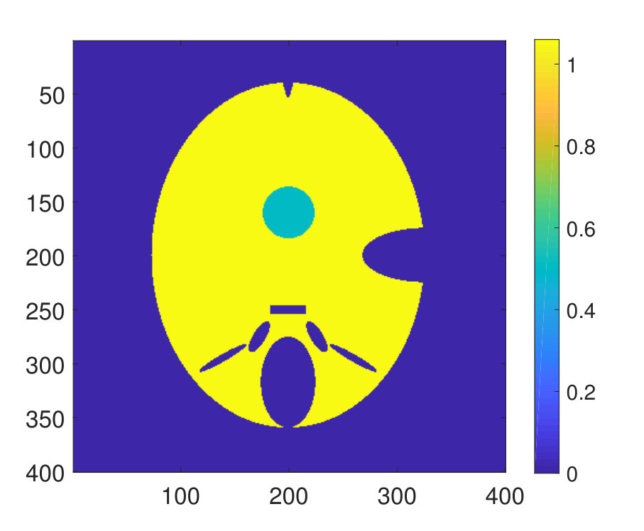 Figure 29
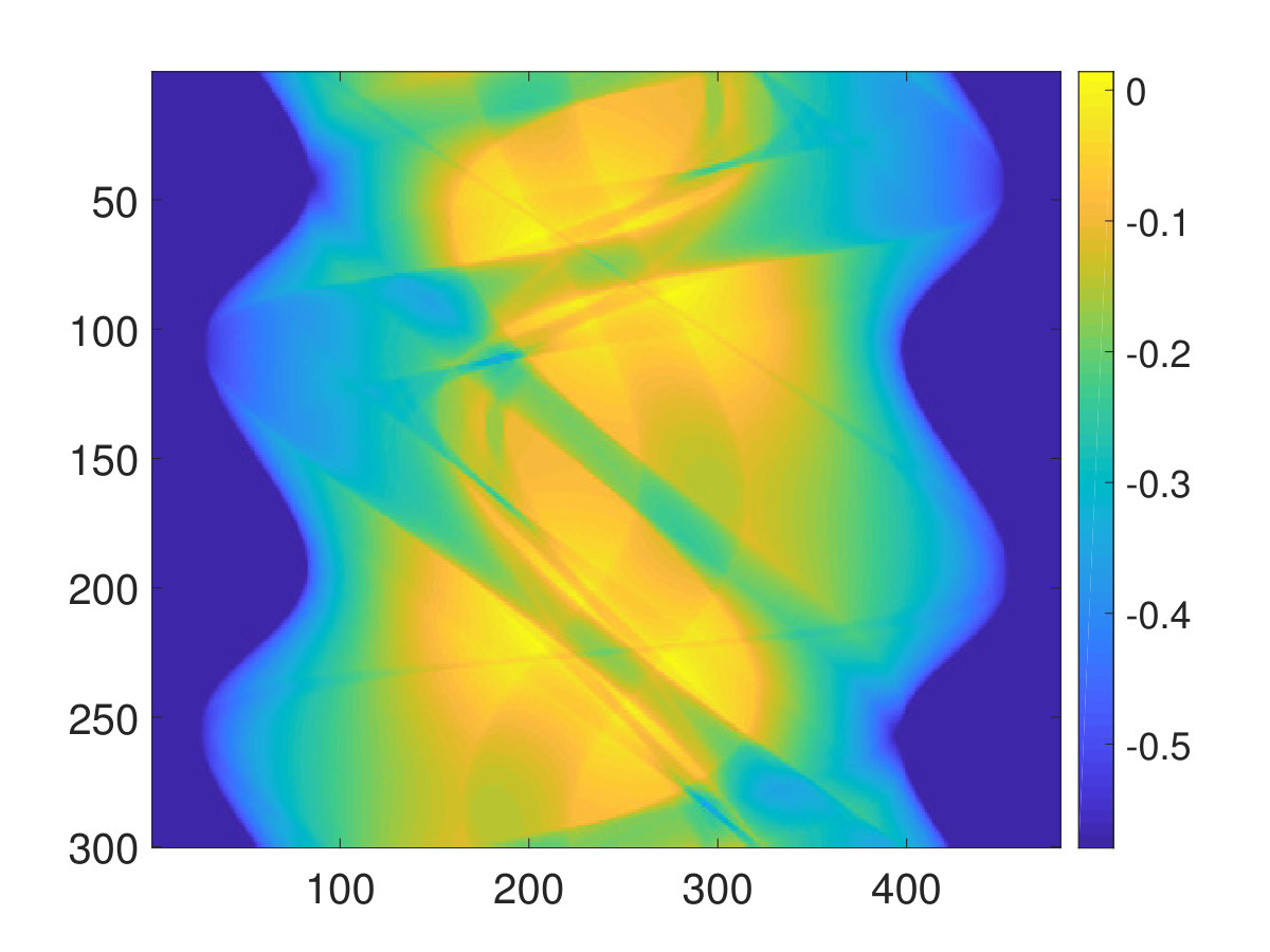 Figure 30
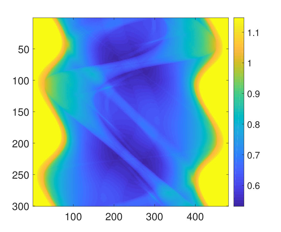 Figure 31
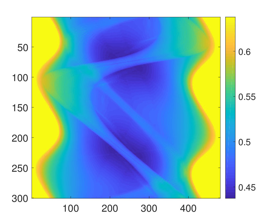 Figure 32
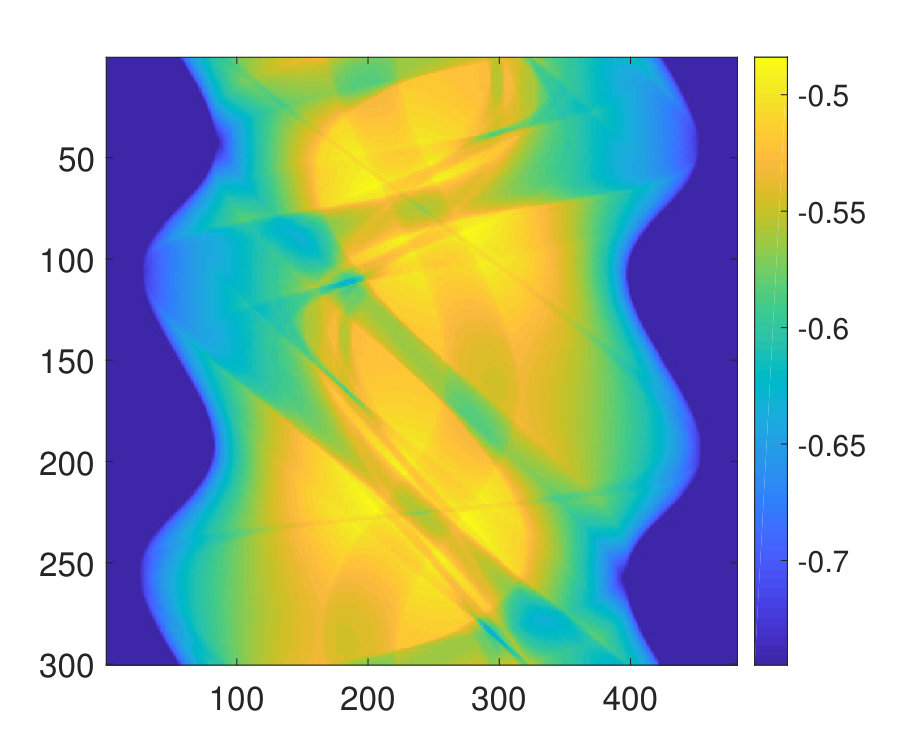 Figure 33
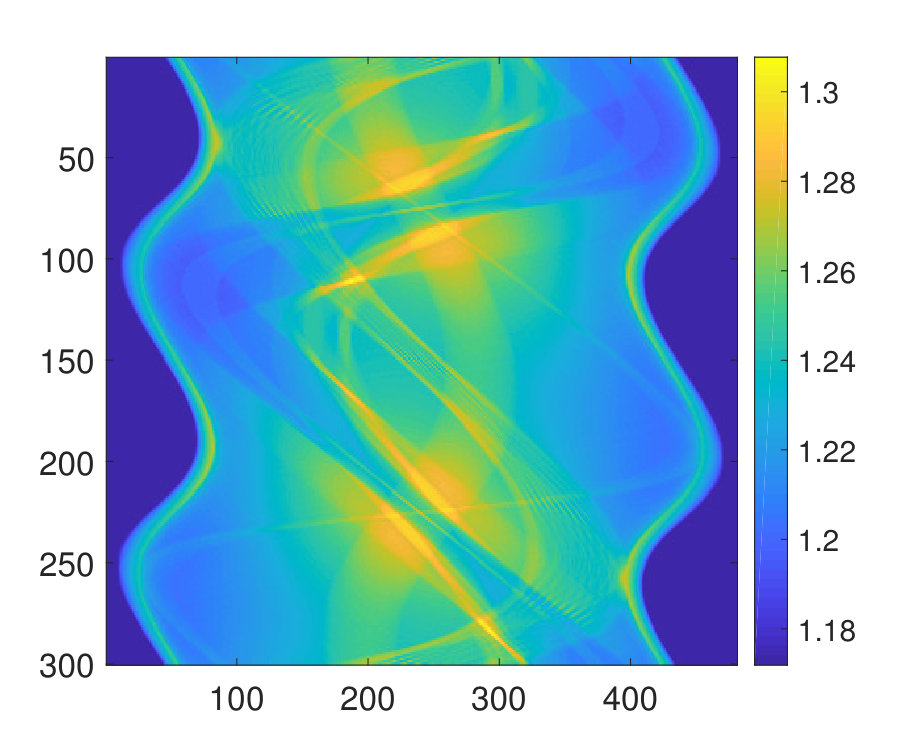 Figure 34
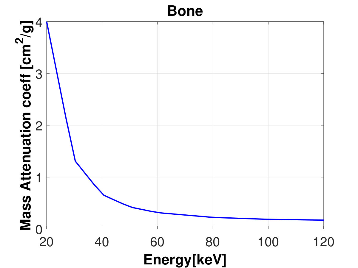 Figure 35
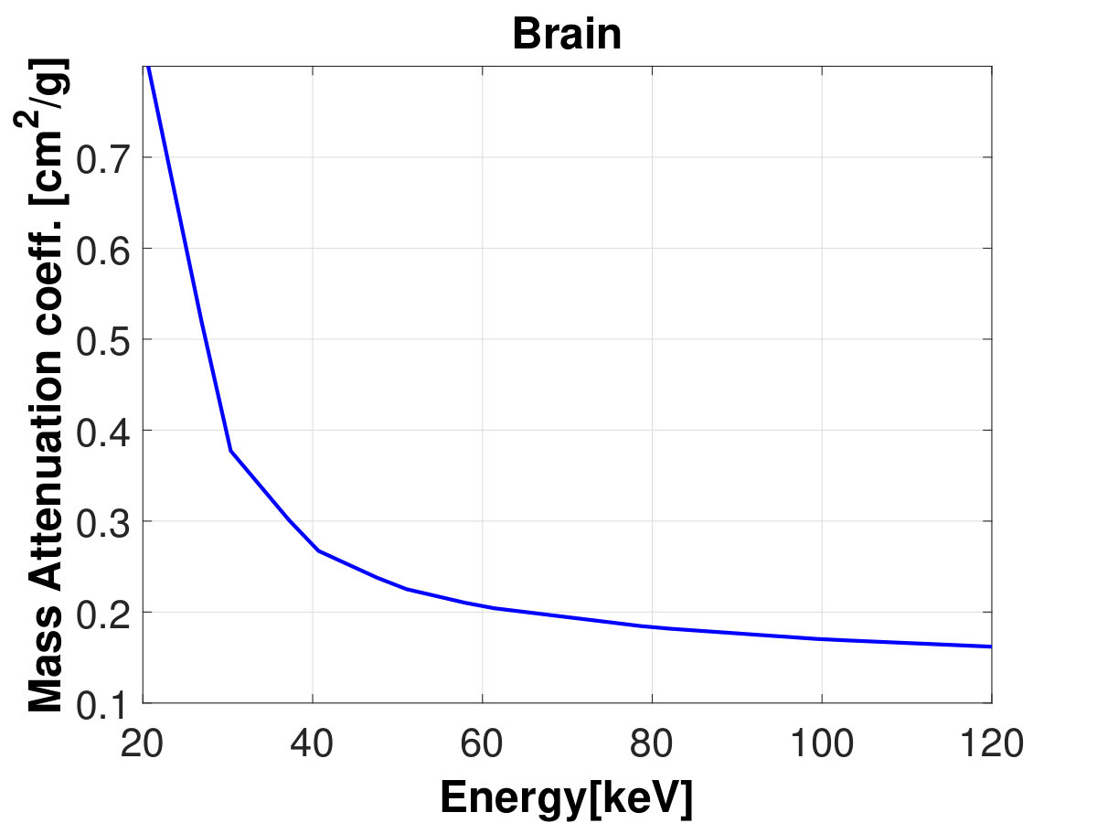 Figure 36
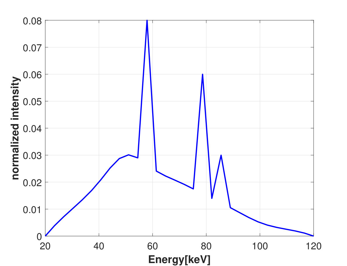 Figure 37
Peer Reviews
No public reviews on file for this paper yet. If you reviewed it on a platform where reviews are public (OpenReview, ICLR, NeurIPS, ICML), you can paste yours below so the community can read it here.
Videos
No videos yet. Explain this paper in a talk, walkthrough, or lecture? Add one.
Analysis of the Block Coordinate Descent Method for Linear Ill-Posed Problems
Simon Rabanser
Department of Mathematics, University of Innsbruck
Technikerstrasse 13, 6020 Innsbruck, Austria
E-mail: [email protected]
Lukas Neumann
Institute of Basic Sciences in Engineering Science, University of Innsbruck
Technikerstrasse 13, 6020 Innsbruck, Austria
E-mail: [email protected]
Markus Haltmeier
Department of Mathematics, University of Innsbruck
Technikerstrasse 13, 6020 Innsbruck, Austria
E-mail: [email protected]
Abstract
Block coordinate descent (BCD) methods approach optimization problems by performing gradient steps along alternating subgroups of coordinates. This is in contrast to full gradient descent, where a gradient step updates all coordinates simultaneously. BCD has been demonstrated to accelerate the gradient method in many practical large-scale applications. Despite its success no convergence analysis for inverse problems is known so far. In this paper, we investigate the BCD method for solving linear inverse problems. As main theoretical result, we show that for operators having a particular tensor product form, the BCD method combined with an appropriate stopping criterion yields a convergent regularization method. To illustrate the theory, we perform numerical experiments comparing the BCD and the full gradient descent method for a system of integral equations. We also present numerical tests for a non-linear inverse problem not covered by our theory, namely one-step inversion in multi-spectral X-ray tomography.
Keywords: ill-posed problems, convergence analysis, regularization theory, coordinate descent, multi-spectral CT
MSC2010: 65J20, 44A12, 47J06.
1 Introduction
We consider the solution of inverse problems of the form
[TABLE]
by block coordinate gradient descent (BCD) methods. Here is a linear forward operator between Hilbert spaces and . Moreover, is the vector of blocks of unknown variables, are the given noisy data, and denotes the data perturbation that satisfies for some noise level .
For many inverse problems, the individual blocks arise in a natural manner and might correspond to , where are functions modeling unknown spatially varying parameter distributions. The blocks might also be formed by applying domain decomposition to a single function , and defining as the restriction of to .
1.1 Iterative regularization methods
The characteristic feature of inverse problems is their ill-posedness which means that the solution of (1.1) is unstable with respect to data perturbations. In such a situation, one has to apply regularization methods to obtain solutions in a stable way. There are at least two basic classes of regularization methods: iterative regularization and variational regularization [6, 23]. In this paper we consider iterative regularization and introduce and analyze BCD as new member of this class of regularization methods.
The most established iterative regularization approaches for inverse problems are the Landweber iteration and its variants [11, 14, 9, 19]
[TABLE]
where is an initial guess, is the step size and denotes the adjoint of . If the step size is taken constant, then (1.2) is the Landweber iteration [14, 9]. Other step size rules yield the steepest descent and the minimal error method [20] or a more recent variant analyzed in [19]. Kaczmarz type variants of (1.2) for systems of ill-posed equations have been analyzed in [5, 8, 7, 13, 15, 16]. Kaczmarz methods make use of a product structure of the image space , and are in this sense dual to BCD methods which exploit the product structure of the pre-image space .
We consider the product form , where the forward operator can be written as . As a consequence, the Landweber iteration takes the form
[TABLE]
We see that each iterative update requires computing separate updates, one for each of the blocks.
1.2 Block coordinate descent (BCD)
In order to simplify the iterative update in (1.3), a natural idea is to update only a single block in each iteration. This results in the BCD iteration
[TABLE]
where the control selects the block that is updated in the th iteration. If we apply the BCD iteration to exact data where , we write instead of . Rigorously studying the iteration (1.4) in the context of ill-posed problems is the main aim of this paper. To guarantee convergence in the noisy case we will slightly modify the update rule of the BCD iteration by including a loping strategy which skips the th iterative step if a certain residual term is sufficiently small (see Definition 2.4). Under the reasonable assumption that the complexity of evaluating is essentially -times the complexity of evaluating , then one step of the Landweber Method has complexity , whereas one step of the BCD method has complexity . For the special form of considered in the following section, the complexity of one step of the BCD method even reduces to ; see Remark 2.2.
Note that the iteration (1.4) arises by applying the block gradient descent method, well known in optimization [3, 18, 22, 24], to the residual functional . In a finite dimensional setting, BCD and other coordinate descent type methods are well studied. However, existing convergence results mostly analyze convergence in the objective value. This only implies convergence in pre-image space, if the residual functional is strongly convex. Strong convexity does not hold for ill-posed problems. Therefore, existing convergence results and methods cannot be applied to ill-posed inverse problems. Note that removing the strict convexity assumption can also also be achieved by coupling the BCD method with a proximal term; see [4] and the references therein.
To the best of our knowledge, no convergence result for (1.4) in the ill-posed setting is available. As the main contribution in this paper we will present a convergence analysis of BCD applicable to the ill-posed case. We show that under assumptions specified in Section 2, for operators having a particular tensor product form, the BCD iteration yields a regularization method for solving ill-posed linear problems.
1.3 Outline
This paper is organized as follows. In Section 2 we present the main assumptions made in this paper, derive an auxiliary results and introduce the loping strategy. In Section 3 we present the convergence analysis. In the exact data case, we show that the BCD iteration converges to a solution of the given equation as . In the noisy data case we show that the stopping index of the loping BCD iteration is finite and the corresponding iterates converge to as . To illustrate the theory, in Section 4 we compare the BCD method with the gradient method for a system of integral equations. Additionally, in Section 5 we consider a non-linear example not covered by our theory, namely one-step inversion in multi-spectral X-ray tomography [21, 12, 1, 2]. The paper concludes with a short discussion presented in Section 6.
2 Preliminaries
In this section we formulate the main assumptions and derive basic results that we will use in the convergence analysis presented in Section 3.
Note that for any Hilbert space we can write . For any we define the projection operators
[TABLE]
where denotes the th standard basis vector in , defined by and for . Using (2.1), the BCD method (1.4) can be written in the compact form
[TABLE]
Here is the selected block at the th iteration, is the step size, and is some initial guess. Recall that in the case of exact data we write instead of .
2.1 Main assumptions
We note that the main difficulty we encountered in the convergence analysis of the BCD method for ill-posed problems is that even for exact data , the error is not monotonically decreasing, except for some very special cases. This can be easily verified for linear operators in . On the other hand, the BCD is monotonically decreasing in the objective value, which is used in existing convergence theory for optimization problems [3, 18, 22, 24]. However, this cannot be used directly for the convergence analysis in the ill-posed setting where the value of the residual functional gives no bounds for the error .
We present a complete convergence analysis under the following assumption that allows to separate the difficulties due to the ill-posedness and due to the non-monotonicity.
Assumption 2.1** (Main conditions for the convergence analysis).**
**
- (A1)
, are Hilbert spaces of the form , with . 2. (A2)
* has the form , where*
* is bounded linear;*
* has rank and non-vanishing columns ;* 3. (A3)
The control satisfies
.
Let us introduce the operators
[TABLE]
In a similar manner we denote and . Then we have .
To overcome the above mentioned obstacles in the convergence analysis we will study the auxiliary sequence which, by linearity, satisfies
[TABLE]
Here we have set
[TABLE]
We will also use the notation . As an important auxiliary result we will show monotonicity for . This allows us to show that the BCD method combined with a loping strategy is a convergent regularization method. In fact, this is the reason for requiring the forward operator to have the particular tensor product form specified in assumption (A2). The convergence analysis in the more general setting is still an open and challenging problem.
Note that the assumption is only necessary for the convergence of implying convergence of . In the case that has arbitrary rank, the main convergence results still hold true for the semi-norm in place of the norm .
Remark 2.2** (Numerical complexity).**
For the considered form and a cyclic control , one cycle of updates with the BCD method for has essentially the same numerical complexity as one iteration with the Landweber iteration. To see this, we implement the BCD method in the following manner:
- (S1)
Initialization: do
**
. 2. (S2)
Updates: do
**
.
Complexity of the above procedure is dominate by the evaluation of , and the evaluation of , . Unless is very large (or evaluating , is cheap), for typical inverse problems, the dominating parts are , . This shows that the complexity of one cycle of the BCD iteration in fact is similar to the complexity of one iteration of the Landweber iteration.
2.2 Monotonicity
The following lemma is an important auxiliary result, which will be used at several places throughout this article.
Lemma 2.3** (Monotonicity).**
Let satisfy and set
[TABLE]
Then, the following estimate holds:
[TABLE]
In particular, if and and if the step size is chosen such that
[TABLE]
then .
Proof.
Equation (2.3) implies
[TABLE]
We have
[TABLE]
By combining (2.8) with the above estimate, we obtain
[TABLE]
which is the desired estimate (2.6). If is chosen according to (2.7), then the right hand side in inequality (2.6) is less or equal to 0, which implies . ∎
2.3 Loping BCD and discrepancy principle
From Lemma 2.3 we see that if the residual term satisfies (2.5), then the error is decreasing. In the case that (2.5) does not hold, then an iterative update might increase the value of . Following a similar strategy introduced in [8, 5] for Kaczmarz type iterative method we therefore modify (2.2) by introducing a loping strategy as follows.
Definition 2.4** (Loping BCD).**
We define the loping BCD method by
[TABLE]
where is as in Equation (2.5), and
[TABLE]
In the case of exact data, we have and the loping BCD iteration reduces to the standard BCD. In the noisy data case the loping parameters ensure that no update is made if we cannot guarantee that an update would decrease . Note that the choice of as in (2.11) implies that condition (2.5) is satisfied whenever we have . For the loping BCD, Lemma 2.3 therefore implies that the error term is in fact monotonically decreasing. Moreover, we can show the following.
Lemma 2.5** (Summability of squared residuals).**
Let satisfy . Then the residuals of the loping BCD iteration (2.9), (2.10) satisfy
[TABLE]
where, , , are chosen such that
- (S1)
* with ;* 2. (S2)
; 3. (S3)
.
Proof.
We first show
[TABLE]
If , then and and therefore (2.13) holds with equality. If , application of Lemma 2.3, (S2) and (S1) yield
[TABLE]
This shows (2.13) with in (2.10).
Summing (2.13) over all and using (S3) we obtain
[TABLE]
which shows (2.12) after dividing by . ∎
Remark 2.6**.**
Note the conditions for the step sizes in Lemma 2.5 are inspired by [19], where a new step size rule for the gradient method for ill-posed problems has been introduced. From the definitions of we obtain . Moreover, recall that . Consequently,
[TABLE]
This implies that we can choose the step sizes bounded from below. In particular, (2.12) holds for any constant step size choice .
3 Convergence Analysis of the BCD method
Throughout the following, let Assumption 2.1 be satisfied. Moreover, we assume that the step sizes satisfy for some numbers independent of the iteration index and the noise level , and that (S1)-(S3) in Lemma 2.5 hold.
3.1 Convergence for exact data
In this subsection we show convergence of the BCD iteration in the noise free case. The proof closely follows [5, 13].
Theorem 3.1** (Convergence of BCD for exact data).**
In the exact data case , the BCD iteration defined by (2.2), satisfies , where is the solution of with minimal distance to .
Proof.
Let satisfy and define . We will show that is a Cauchy sequence. For and with and , let be such that
[TABLE]
With we have
[TABLE]
and
[TABLE]
According to Lemma 2.3, the nonnegative sequence is monotonically decreasing and therefore converges to some . Consequently, the last two terms in equations (3.3) and (3.4) converge to for . In order to show that also and converge to zero, we set . Then using the definition of the BCD method in (2.2) for we obtain
[TABLE]
with . Further we obtain
[TABLE]
Substituting the estimate in (3.5), using the inequality and (3.1) one concludes
[TABLE]
where we defined . Finally, we have
[TABLE]
Because of Lemma 2.5, the last sum converges to zero for which implies . Similarly, one shows . Therefore, is Cauchy sequence and tends to an element with . Because has rank and , the element is a solution of . Further,
[TABLE]
Because is closed, its follows that . Since is the only solution for which the latter holds true, we obtain . ∎
3.2 Convergence for noisy data
In the noisy data case, we consider the loping version of the BCD. The iteration is terminated when for the first time all are equal within a cycle. That is, we stop the iteration at
[TABLE]
To simplify the notation, we assume that for all . We first show that the stopping index is always finite.
Proposition 3.2** (Existence of stopping index).**
If , then the stopping index defined in (3.9) is finite, and we have
[TABLE]
Proof.
If for every , there exists such that , then from Lemma 2.5 we obtain
[TABLE]
where is a lower bound of . The right hand side of (3.11) tends to infinity, which gives a contradiction. Consequently, the set is nonempty and therefore contains a finite minimal element.
To prove (3.10) note that the finiteness of the stopping index and the definition of the loping BCD implies for . The assumption (A3) on the control sequence thus gives (3.10). ∎
We call the step size selection continuous at if for all we have
[TABLE]
An example for a continuous step size selection is the constant strep size . The next auxiliary result shows that the continuity of the step size selection implies continuity of at .
Lemma 3.3** (Continuity of the BCD iteration at ).**
Suppose the step selection is continuous at , and define
[TABLE]
Then, for all , we have
[TABLE]
Moreover, , as .
Proof.
We prove Lemma 3.3 by induction. Assume and that (3.13) holds for all . First we note that (3.13) implies , as . For the proof of (3.13) we consider two cases. In the first case, , we have
[TABLE]
In the second case, , we have . Consequently,
[TABLE]
Now (3.13) follows from the continuity of , and the induction hypothesis implying . ∎
Theorem 3.4** (Convergence of the loping BCD for noisy data).**
Suppose the step selection is continuous at . Let converge to [math] and let be a sequence of noisy data with . Let be defined by the loping BCD iteration with data and stopped at according to (3.9). Then , where is the solution of with minimal distance to .
Proof.
From Lemma 3.3 and the continuity of we have, for any , that and as .
To show that , we first assume that has a finite accumulation point . Without loss of generality we may assume that for all . From Proposition 3.2 we know that . By taking the limit , we obtain . Consequently, and as . It remains to consider the case where as . To that end let . Without loss of generality we assume that is monotonically increasing. According to Theorem 3.1 we can choose such that . Equation (3.13) implies that there exists such that for all . Together with the monotonicity we obtain
[TABLE]
Because is non-singular, this shows as . ∎
4 Example: System of linear integral equation
In this section we compare the BCD method to the standard Landweber method for an elementary system of linear integral equations.
4.1 Forward problem
Consider the integration operator defined by
[TABLE]
According to the Cauchy-Schwarz inequality, we have
[TABLE]
for all , which shows that is a well-defined linear bounded operator. Using the operator we consider the following forward model applied to a vector of functions .
Definition 4.1**.**
For and given matrix of rank , we define the forward operator
[TABLE]
According to our general notion we have and the theory presented in the previous section can be applied for solving the inverse problem . Note that this equation clearly is ill-posed because the range of is non-closed (and equal to the Sobolev space of all weakly differentiable functions vanishing at [math].)
More generally, one could replace the integration operator by any bounded (integral) operator with non-closed range.
4.2 Reconstruction results
For all presented numerical results we use and take with
[TABLE]
We discretize with the composite trapezoidal rule using intervals such that the data and the unknowns are elements in . The true unknown and the noisy data are shown in Figure 4.1. The exact data have been computed via numerical integration followed by application of . Subsequently we computed noisy data by adding random white noise to with a standard deviation of . The resulting relative data errors are , and , respectively.
Reconstruction using the BCD and Landweber methods from simulated data are shown in Figure 4.2. For each case we have used the maximum constant step-size, that lead to stable reconstruction. We evaluate the reconstruction error (norm of ) in terms of the standard 2-norm and in the -norm ,
[TABLE]
respectively. As we can see from the bottom row in Figure 4.2, measured in both norms, the reconstruction error of the BCD is smaller than the error of Landweber iteration.
Figure 4.3 shows reconstruction results for nosy data. Again, the error in the BCD method decreases faster than the one of the Landweber method. The BCD therefore requires less cycles than the Landweber method. Moreover, in the middle column of Figure 4.3 we illustrate the need for the loping (or another regularization strategy). Without loping, the BCD iteration as well as the Landweber iteration start to diverge after around 2000 iterations. With loping (for the BCD method) and the with the discrepancy principle (for the Landweber method) both iterations stop. (Note that here we only show the error in the -norm and that the Landweber method is monotonically decreasing in the -norm when using the discrepancy principle.) Finally, the bottom row in Figure 4.3 shows that the reconstruction error for the BCD iteration is not monotonically decreasing in the standard norm, whereas in the -norm it is.
5 A nonlinear test: Multi-spectral X-ray tomography
In this section we apply a nonlinear generalization of the BCD and the Landweber iteration to one-step inversion in multi-spectral X-ray tomography. In particular, for nonlinear operators in place of linear ones, we use the following generalization of the BCD iteration
[TABLE]
Note that such problems are not covered be our theoretical analysis. We consider extending our theory to this class of examples a particularly interesting topic of future research.
In the following we denote by the disc with radius centered at the origin. We define the fan beam Radon transform of a function supported in by
[TABLE]
It can be easily verified that the fan beam Radon transform is linear and continuous [17].
5.1 Mathematical modeling
We assume that the tissue is composed of different materials each of them having a different energy dependent X-ray attenuation coefficient with . The combined X-ray attenuation coefficient is then given by
[TABLE]
where is the fractional density map of the th material. Our goal is to determine the fractional density maps from multi-spectral X-ray transmission measurements.
The energy sensitive X-ray transmission measurements result in the intensity [2]
[TABLE]
Here denotes the energy window where the measurement is made and is the product of X-ray beam spectrum intensity and detector sensitivity. We assume the detector sensitivity to be constant and that the spectrum is known for energies ranging from to covering any energy window. The spectrum used for the numerical results is the same as in [1, 2] and shown in Figure 5.1.
In order to recover multiple material densities, we use multiple energy windows. We choose the same number of spectral windows as we have different materials. Moreover, to simplify the mathematical formulation we uniformly discretize the energy variable, 20\text{,}\mathrm{keV}120\text{,}\mathrm{keV}$$. The X-ray measurements corresponding to the th energy window is given by
[TABLE]
Here model discrete energy windows, is the discretized beam spectrum intensity, and 120\text{,}\mathrm{keV}. Summarizing the above we define the following forward operator.
Definition 5.1** (Multi-spectral X-ray measurement operator).**
The measurement operator with respect to the energy windows is given by
[TABLE]
We can decompose the operator in the form
[TABLE]
where
.
The operators are linear and bounded. To show the continuity and differentiability of we have to verify that is continuous and differentiable.
Proposition 5.2** (Continuity and differentiability of ).**
The operator is continuous and Fréchet differentiable. For we have
[TABLE]
with
[TABLE]
Proof.
One only has to verify that is continuous and Fréchet differentiable on with derivative given by . For that purpose, let which in particular implies its point wise convergence. Therefore
[TABLE]
This shows (5.9), and (5.8) follows by the chain rule. ∎
In the context of the BCD method, the fractional density maps play the roles of the blocks . The form (5.7) of the forward operator has some similarity with the form that we used in the theoretical analysis of the BCD method, in the sense that the infinite dimensional smoothing operator is applied to several channels of a function. However, so far we have not been able to perform an analysis accounting for the non-linearity. Additionally, we apply a preconditioning technique as outlined in the following subsection. Extending the convergence analysis of BCD such that it applies to multi-spectral CT is subject of future research.
5.2 Logarithmic scaling and preconditioning
The energy dependence of the mass-attenuation coefficient of different materials can be quite similar. In order to enhance the dependence on the different materials we propose a logarithmic scaling and preconditioning technique (different from [2]). For simplicity we consider only the case , the general case can be treated in a similar manner.
The proposed preconditioned logarithmic data take the form
[TABLE]
where are the unknowns and , , , are parameters. Moreover, recall that and are the X-ray intensities defined by (5.6) corresponding to modeling the discrete energy windows. The preconditioned inverse problem consists in solving the system
[TABLE]
where are data perturbed by noise .
In order to solve the equations in (5.11), (5.12) with the BCD method we define the residual functionals
[TABLE]
Application of the BCD method requires the adjoint gradient of and , that we compute next.
Proposition 5.3** (Derivative of the preconditioned residuals).**
Let . The directional derivatives of and at in direction are given by
[TABLE]
Proof.
This follows from the chain rule. ∎
From Proposition 5.3 we conclude that the partial gradients of the residual functionals are given by
[TABLE]
These expressions will be used for the implementations of the BCD as well as the Landweber method applied to the preconditioned system (5.11).
5.3 Numerical implementation
For all our experiments we used fan beam geometry. Each channel of the discrete phantom has size . We discretized using 300 detector positions equidistantly distributed on . For each detector position we compute line integrals for uniformly distributed angles in the interval . To actually compute we used the trapezoidal rule and linear interpolation where we discretized the line integral using 400 equidistant sampling points in the interval . The adjoint is evaluated using the standard backprojection algorithm with linear interpolation. We used equidistant discrete energy positions from to .
For our numerical studies we apply one-step inversion in multi-spectral CT tomography to reconstruct a head phantom composed of two different material map derived from FORBID head. The phantom is shown in Figure 5.2 and consists of the pair , where corresponds to the fractional density of the brain and to the fractional density of the bone material. We slightly modified the FORBID head phantom by inserting a disk with value in both components to demonstrate that the method can actually reconstruct mixed material distributions. The mass attenuation coefficients of the material maps (bone and brain) are taken from NIST tables [10] and are shown in Figure 5.3.
Figure 5.4 shows the data used for image reconstruction. In the first row original data according to Definition 5.1 are plotted, where the indices and corresponds to energy windows 20\text{,}\mathrm{k}\mathrm{e}\mathrm{V}70\text{,}\mathrm{k}\mathrm{e}\mathrm{V} and 70\text{,}\mathrm{k}\mathrm{e}\mathrm{V}120\text{,}\mathrm{k}\mathrm{e}\mathrm{V}, respectively. One can observe, the data for both energy windows look quite similar. This is because of the similar energy dependence of the mass attenuation coefficients for and ; compare Figure 5.3. For this reason, we make use of the proposed scaling and preconditioning outlined in Section 5.2. The second row shows the preconditioned data we use for the reconstruction. For comparison purpose, the last row in Figure 5.4 shows the negative logarithm of the X-ray intensities for the full energy window, with in each case containing only one of the material maps. We have chosen the constants , , and in such a way that each of the modified data blocks highlights different aspects of the material maps. Note that we have selected the constants for data of a very different phantom in order to avoid inverse crime.
5.4 Numerical results
For the following results we compare the performance of the BCD method with the standard gradient method as reference method. We use a cyclic control and constant step sizes for both methods. Note that for the BCD as well as the Landweber method we included a positivity constraint. Figure 5.5 shows reconstruction results for the bone and brain material map. Due to the applied logarithmic scaling and preconditioning, both methods are able to separate the materials after a reasonable number of iterations. One observes that even the mixed part can be reconstructed as well.
Figure 5.6 shows the relative squared reconstruction errors
[TABLE]
of the bone and the brain map using the Landweber method and the BCD method. The horizontal axes show the number of iterations in the Landweber method and the number of cycles (number of iterations divided by the number of blocks) in the BCD method. A cycle for the BCD method has the same numerical complexity as one iteration for the Landweber method. The BCD method delivers a lower relative error for the brain map, the relative error of the reconstruction for the bone map is similar for both methods.
Reconstruction results for noisy data are shown in Figure 5.7. To generate the noisy data, we added Gaussian white noise with standard deviation equal to of the maximal value of the exact data. In order to maintain stability of both iterations we stopped the Landweber iteration after iterations, accordingly the BCD-method is stopped after cycles. The relative squared reconstruction error is shown in Figure 5.8. Again, the BCD method is roughly a factor two faster than the Landweber method in recovering the brain map. For recovering the bone map, both methods are equally fast. We associate this different behavior to the particular form of preconditioning. As can be seen from the second line in Figure 5.4, both preconditioned data pairs contain significant parts of the data corresponding to the brain whereas the bone data is mainly contained in the second one. Investigating optimal weights for the preconditioning is an interesting aspect of future work.
6 Conclusion
In this paper we analyzed the BCD (block coordinate descent) method for linear inverse problems. For a particular tensor product form we have shown that the BCD method combined with an appropriate loping and stopping strategy is a convergent regularization method for ill-posed inverse problems. The analysis in the present paper applies to operators having the tensor product form , where and is linear. We presented two examples for numerically solving ill-posed problems with the BCD method. The first one is concerns a system of linear integral equations that is covered by our theory. As an outlook we applied the BCD method to an example not covered by our theory, namely one-step inversion in multi-spectral X-ray computed tomography.
Future work will be done to extend our analysis of the BCD method to more general forward operators, in particular non-linear problems including examples like multi-spectral CT. This is challenging as the BCD is not monotone in the reconstruction error . However, we believe that the technique introduced in this paper of finding a suitable norm where monotonicity holds can be extended to more general situations.
Acknowledgments
The work Markus Haltmeier has been supported by the Austrian Science Fund (FWF), project P 30747-N32. Simon Rabanser acknowledges support of the Austrian Academy of Sciences (ÖAW) via the DOC Fellowship Programme. The authors thank the anonymous reviewers for valuable comments that helped to significantly improve the manuscript.
The reference list from the paper itself. Each links out to its DOI / PubMed record.
- 1[1] H. Atak and P. M. Shikhaliev. Dual energy ct with photon counting and dual source systems: comparative evaluation. Phys. Med. Biol. , 60(23):8949, 2015.
- 2[2] R. F. Barber, E. Y. Sidky, T. G. Schmidt, and X. Pan. An algorithm for constrained one-step inversion of spectral CT data. Phys. Med. Biol. , 61(10):3784, 2016.
- 3[3] A. Beck and L. Tetruashvili. On the convergence of block coordinate descent type methods. SIAM J. Optim , 23(4):2037–2060, 2013.
- 4[4] J. Bolte, S. Sabach, and M. Teboulle. Proximal alternating linearized minimization for nonconvex and nonsmooth problems. Mathematical Programming , 146(1-2):459–494, 2014.
- 5[5] A. De Cezaro, M. Haltmeier, A. Leitão, and O. Scherzer. On steepest-descent-Kaczmarz methods for regularizing systems of nonlinear ill-posed equations. Appl. Math. Comput. , 202(2):596–607, 2008.
- 6[6] H. Engl, M. Hanke, and A. Neubauer. Regularization of inverse problems , volume 375. Springer Science & Business Media, 1996.
- 7[7] M Haltmeier. Convergence analysis of a block iterative version of the loping Landweber-Kaczmarz iteration. Nonlinear Anal. , 71(12):e 2912–e 2919, 2009.
- 8[8] M. Haltmeier, A. Leitão, and O. Scherzer. Kaczmarz methods for regularizing nonlinear ill-posed equations. I. Convergence analysis. Inverse Probl. Imaging , 1(2):289–298, 2007.