Heavy particles in a persistent random flow with traps
J. Meibohm, B. Mehlig

TL;DR
This paper models heavy particles in a one-dimensional compressible fluid with persistent Gaussian velocity fields, analyzing trapping, Lyapunov exponents, and caustic formation, with implications for higher-dimensional systems.
Contribution
It introduces a novel analytical framework for understanding particle trapping and caustic formation in a 1D compressible flow with weak inertia.
Findings
Particles tend to accumulate in trapping regions.
Analytical expressions for Lyapunov exponents and caustic rates are derived.
Numerical simulations confirm the analytical predictions.
Abstract
We study a one-dimensional model for heavy particles in a compressible fluid. The fluid-velocity field is modelled by a persistent Gaussian random function, and the particles are assumed to be weakly inertial. Since one-dimensional fluid-velocity fields are always compressible, the model exhibits spatial trapping regions where particles tend to accumulate. We determine the statistics of fluid-velocity gradients in the vicinity of these traps and show how this allows to determine the spatial Lyapunov exponent and the rate of caustic formation. We compare our analytical results with numerical simulations of the model and explore the limits of validity of the theory. Finally, we discuss implications for higher-dimensional systems.
Click any figure to enlarge with its caption.
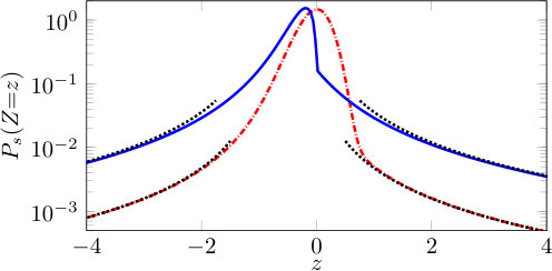 Figure 1
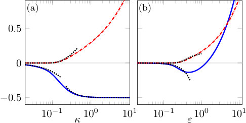 Figure 2
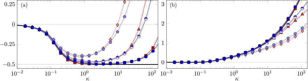 Figure 3
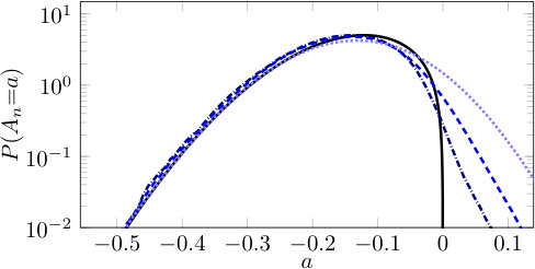 Figure 4
Peer Reviews
No public reviews on file for this paper yet. If you reviewed it on a platform where reviews are public (OpenReview, ICLR, NeurIPS, ICML), you can paste yours below so the community can read it here.
Videos
No videos yet. Explain this paper in a talk, walkthrough, or lecture? Add one.
Heavy particles in a persistent random flow with traps
J. Meibohm
Department of Physics, Gothenburg University, SE-41296 Gothenburg, Sweden
B. Mehlig
Department of Physics, Gothenburg University, SE-41296 Gothenburg, Sweden
Abstract
We study a one-dimensional model for heavy particles in a compressible fluid. The fluid-velocity field is modelled by a persistent Gaussian random function, and the particles are assumed to be weakly inertial. Since one-dimensional fluid-velocity fields are always compressible, the model exhibits spatial trapping regions where particles tend to accumulate. We determine the statistics of fluid-velocity gradients in the vicinity of these traps and show how this allows to determine the spatial Lyapunov exponent and the rate of caustic formation. We compare our analytical results with numerical simulations of the model and explore the limits of validity of the theory. Finally, we discuss implications for higher-dimensional systems.
pacs:
05.40.-a,47.55.Kf,47.27.eb
I Introduction
Turbulent fluids in Nature and Technology often contain small particles whose density is larger than that of the carrier fluid. Examples are sprays, water droplets in turbulent clouds, and dust in the exhaust of combustion engines. It is a common observation that these particles do not distribute homogeneously in space, but instead form regions of high and low concentration on small scales. This effect is referred to as spatial clustering Bec (2003); Wilkinson and Mehlig (2003); Gustavsson and Mehlig (2016), and it is a consequence of the interaction of the particles with the turbulent fluid. Hence, any attempt to describe these systems must take into account the turbulent fluctuations, a challenging problem by itself.
Recently, much progress has been made in explaining and quantifying spatial clustering of heavy particles in turbulence, using statistical models. See Ref. Gustavsson and Mehlig (2016) for a recent review. Such models approximate the turbulent fluid-velocity fluctuations below the smallest scales of turbulence, called the dissipative range, in terms of random velocity fields with prescribed statistics. Clearly, these random velocity fields lack the complexity of real turbulence. Remarkably, however, such statistical models often reproduce the dynamics of the immersed particles and the statistical properties of their spatial distribution qualitatively, and in some cases even quantitatively. Statistical models allow for much simpler numerical simulations and even admit analytical treatment in limiting cases Wilkinson and Mehlig (2003); Gustavsson and Mehlig (2016); Falkovich et al. (2007). The models typically depend on two parameters, the Kubo number Ku, which is a measure of the persistence of the flow, and the Stokes number St, which measures the importance of particle inertia in the fluid-particle system.
Spatial clustering is often characterised in terms of the spatial Lyapunov exponents , Sommerer and Ott (1993); Gustavsson and Mehlig (2016). These exponents measure the rates at which particles approach or diverge, in the long-time limit. Because heavy particles are not constrained to follow the flow, their dynamics takes place in -dimensional phase space, while their spatial concentration is measured in the -dimensional coordinate space. As a consequence, the spatial distribution of the particles exhibits singularities, so-called caustics, which contribute to the spatial clustering of the particles Falkovich et al. (2002); Wilkinson and Mehlig (2005); Wilkinson et al. (2006); Falkovich et al. (2007). One therefore identifies the rate of formation of these singularities, the rate of caustic formation , as a second important observable.
A well-studied limiting case of the statistical model is the so-called white-noise limit, describing the dynamics of very heavy particles in a rapidly fluctuating fluid-velocity field. In terms of the dimensionless parameters, this limit corresponds to and so that remains constant Gustavsson and Mehlig (2016). An important property of white-noise models is that they depend solely on a single parameter, , where is a function of the spatial dimension and the compressibility parameter of the underlying flow field. The parameter takes the role of an inertia parameter in the white-noise model, similar to the Stokes number St in statistical models at finite values of Ku Gustavsson and Mehlig (2016). In the white-noise limit in one spatial dimension, and can be computed analytically as a function of Wilkinson and Mehlig (2003).
In this Paper, we describe a second limiting case of the statistical model, the persistent-flow limit. This limit describes weakly inertial, heavy particles in a very persistent flow, hence the name. The limit is taken by letting and such that the product Ku St stays finite. Similarly to the white-noise limit, the persistent-flow limit turns out to depend on a single inertia parameter , where Gustavsson and Mehlig (2016).
Here, we confine ourselves to the one-dimensional version of the model, , and show that and can be computed analytically in the persistent-flow limit. In one spatial dimension, the random fluid-velocity field is compressible. Because of the high persistence of the flow, compressibility leads to long-lived trapping regions, regions in space where the particles accumulate. We show that the statistics of fluid-velocity gradients in the trapping regions are the crucial ingredient to solving the one-dimensional model.
The Paper is organised as follows: In Sec. II we introduce the model for heavy particles in turbulence and motivate the persistent-flow limit by a detailed analysis of the relevant time scales. Section III contains the statement and the derivation of the analytical results for the spatial Lyapunov exponent and the rate of caustic formation . We compare these results to those obtained in the white-noise limit, and to results of numerical simulations of the statistical model. We draw conclusions and discuss implications for higher-dimensional models in Sec. IV. The Appendix contains an alternative derivation of the main formulae derived in Sec. III.
II Problem formulation
We study a one-dimensional model for the motion of heavy particles in the dissipative range of turbulence, approximating the viscous force on the particle by Stokes drag. The equations of motion for an underdamped small and heavy particle in a viscous fluid are given by
[TABLE]
where is the particle relaxation time, the typical time it takes the particle to relax to the fluid velocity. We model the turbulent fluid velocity by a one-dimensional Gaussian random velocity field with zero mean and correlation Gustavsson and Mehlig (2016)
[TABLE]
In this formulation, the flow field is a function of its root mean square velocity as well as its correlation length and fluid correlation time, and , respectively. Fields in one spatial dimension are always potential, therefore the velocity field is compressible, as mentioned in the Introduction. Models for particles in three-dimensional turbulence, by contrast, usually assume that the flow is incompressible. Further, approximating by a Gaussian random field neglects several characteristic aspects of turbulence such as intermittency and broken time-reversal invariance. It has, however, been shown that the highly-simplified one-dimensional model gives important insights into the dynamics of particles in the dissipative range of turbulence (see Gustavsson and Mehlig (2016) and references therein).
II.1 Relevant time scales
The random velocity field is characterised by two different time scales. In addition to the correlation time , the advection time scale is the typical time it takes an advected (tracer) particle to travel one correlation length . From the three time scales , and , one can define three dimensionless numbers Gustavsson and Mehlig (2016)
[TABLE]
The Kubo number, Ku, measures the persistence of the flow and St is the Stokes number, a measure for particle inertia in the system. The third quantity in expression (3), , compares the particle relaxation time to the advection time and is thus another measure of particle inertia.
In case there is a time-scale separation between and , only one of the two inertia parameters, either St or , needs to be considered. In the white-noise limit Wilkinson and Mehlig (2003, 2005); Wilkinson et al. (2006); Derevyanko et al. (2007); Gustavsson and Mehlig (2016); Pumir and Wilkinson (2016), for instance, the correlation time is the smallest of all time scales. More precisely, this limit is approached if so that the parameter stays finite. In other words, the white-noise limit of Eqs. (1) describes very heavy particles in a rapidly fluctuating flow field. The fluid-velocity gradient becomes a white-noise signal with zero mean and correlation strength . Thus, Eqs. (1) constitute a generalised diffusion process and one can use Fokker-Planck equations to solve the model exactly in one dimension, Wilkinson and Mehlig (2003); Gustavsson and Mehlig (2016). The single relevant dimensionless inertial parameter in the white-noise model is , which is related to the diffusion constant of the generalised diffusion by .
In the persistent-flow limit studied here, by contrast, the correlation time is the largest of the three time scales, i.e., . In terms of dimensionless parameters this limit corresponds to and . The ratio between the remaining time scales is thus given by . Hence, the particle motion and the motion of advected particles take place on time scales much smaller than the correlation time of the fluid. The inertia parameter measures how much the particles detach from the flow, compared to the motion of advected tracers.f
The advection time scale in the statistical model is analogous to the Kolmogorov time in homogeneous isotropic turbulence, defined as . Here is the matrix of fluid-velocity gradients, and is an average along fluid-element paths. Since the Kolmogorov time is the only available microscopic time scale in turbulence, the analogue of (constructed from and ), is commonly used as the inertia parameter in DNS and experiments on the dynamics of heavy particles in turbulence Pergolizzi (2012); Gustavsson and Mehlig (2016).
II.2 One-dimensional model
The observables and are most conveniently studied in terms of the relative dynamics of an ensemble of particle pairs, instead of the single-particle dynamics given in Eqs. (1). The motion of a pair of particles is described by the particle separation and relative velocity , as well as their midpoint position and mean velocity . At separation much smaller than , , a particle pair experiences an essentially linear velocity field. We therefore linearise the equations of motion (1) with respect to . To this end, we introduce the mean flow and the fluid-velocity gradient, . A particle pair at small separation then obeys the linearised equations of motion
[TABLE]
where we have omitted the time dependence of for convenience of notation. The particle-velocity gradient , has the equation of motion Falkovich et al. (2002); Wilkinson and Mehlig (2003); Gustavsson and Mehlig (2016)
[TABLE]
The two equations for , Eqs. (4b), resemble a closed system that is equivalent to the single-particle dynamics (1). Equations (4a) and (5), on the other hand, are not closed as they depend on the variable which enters in the argument of the fluid-velocity gradient.
As both advected tracers and heavy particles move much faster than the fluid changes, , and the fluid-velocity field is compressible, there exist long-lived, stable fixed points of Eqs. (1), and thus Eqs. (4b), where the particles accumulate. These trapping regions are characterised by negative fluid-velocity gradients , and small fluid velocity . Trapping regions appear and disappear randomly with mean rate proportional to Mehlig et al. (2009). When a trapping region vanishes, the trapped particles are driven to a neighbouring trapping region, at a typical distance away.
If we estimate the migration time to the next trapping region by the time it takes for advected tracers to travel one correlation length, . If , on the other hand, the migration time is of the order of the relaxation time of the particles. We conclude that the migration time is of the order of the maximum of these two time scales, .
As trapping regions persist for times , the persistent-flow limit ensures that the time particles spend in trapping regions is much larger than the migration time. Hence, for and we can neglect the disappearance and appearance of stable zeros of and consider the case of an ensemble of particles in an unbounded and frozen Gaussian random velocity field.
Each trapping region in the frozen velocity field is characterised by a constant fluid-velocity gradient , where we index the trapping regions by , for reasons that become clear later. Because different trapping regions are typically a fluid correlation length away from each other, their fluid-velocity gradients can be assumed to be independent and identically distributed.
To obtain the equation of motion for a particle pair in the -trapping region of the flow, we first dedimensionalise Eqs. (4) and (5), so that they do not explicitly dependent on the time scales. That is, we let , , , and . We obtain the dimensionless equations
[TABLE]
In the rest of this Paper, all quantities, including the Lyapunov exponent and the rate of caustic formation , are written in dimensionless form.
The probability density of the random fluid-velocity gradient in the -trapping region, , is given by the distribution of gradients at the zeros of the Gaussian random function , conditioned on that these gradients are negative Gustavsson and Mehlig (2013a). This distribution is obtained by means of the ‘Kac-Rice formula’ Kac (1948); Rice (1944), which allows to compute the density of singular points of random functions. Using that the gradient function is Gaussian distributed, we obtain for the probability density of :
[TABLE]
Eq. (7) shows, that the particle-velocity distribution depends only on the single parameter [Eq. (3)] in the persistent limit. Furthermore it follows from Eq. (7) and the independence of the gradients that
[TABLE]
for all and . Clearly, is the result of strong preferential sampling of negative gradients, due to the accumulation of particles in trapping regions. Eq. (7) shows, in fact, that .
III Results
Using Eqs. (6) and the distribution of we calculate the spatial Lyapunov exponent and the rate of caustic formation . Both quantities can be either obtained directly from the equations of motion for and , Eqs. (6a), or from the steady-state probability density of , . We explain the method using in the following Section and describe the first method in Appendix A. The general idea in both cases is to first compute the respective quantities conditional on a certain gradient realisation, , and then average over all realisations using the probability density given in Eq. (7).
III.1 Steady-state distribution of
We first turn to the computation of the steady-state distribution of . The conditional density obeys the equation
[TABLE]
where the operator is the generator of the Perron-Frobenius operator Cvitanovic et al. (2005) corresponding to the dynamics of in Eq. (6b) given the realisation . The operator reads
[TABLE]
By definition, the conditional steady-state probability density solves and is thus annihilated by ,
[TABLE]
Equation (11) has the solution
[TABLE]
where is the stable fixed point of the dynamics (5) for . The drastic change of at can be understood by noting that Eq. (6b) undergoes a saddle-node bifurcation at that point, generating two fixed points of for . For long times, ends up at the stable of the two fixed points, , in this case. For , on the other hand, there are no fixed points and reaches in a finite time. Because , this case corresponds to two particles overtaking each other, forming a caustic Gustavsson and Mehlig (2016); Falkovich et al. (2002); Wilkinson et al. (2006); Wilkinson and Mehlig (2005). Upon reaching , is immediately reinjected at to ensure also after the caustic event Gustavsson and Mehlig (2011, 2014). We now calculate the steady-state probability density , using
[TABLE]
and substituting the expressions in Eqs. (7) and (12) for and , respectively. We obtain
[TABLE]
where, denotes the indicator function of the set . The steady-state distribution is the sum of two parts, corresponding to the two different solutions of . The first term in Eq. (14) originates from the gradient range , that does not admit caustics, while the second one comes from the gradient range where caustics form. The result for , Eq. (14), as a function of for is shown as the solid line in Fig. 1. The distribution exhibits a peak at and a sharp kink at . For large the distribution has power-law tails , shown as the dotted lines. The steady-state distribution for in the persistent-flow model is thus quite similar to the corresponding quantity in the white-noise model, shown as the dash-dotted line in Fig. 1. We observe a similar peak at small and power-law tails with scaling.
The apparent similarity of the two distributions in these very different limits is due to the similar qualitative dynamics of . In the persistent-flow model, equilibrates at , close to , for the majority of realisations, , hence the peak at . For , repeatedly approaches and returns, leading to the power law tails in the distribution. In the white-noise model, on the other hand, the noisy dynamics of spends most of its time close to the stable fixed point at . Occasionally, however, the gradient history allows to pass the unstable fixed point at and escape to infinity. The -tails of the distribution originate from caustic events . The large- dynamics is universal and independent of the gradient , because the deterministic -term in Eq. (5) dominates for large enough .
III.2 Lyapunov exponent
The spatial Lyapunov exponent
[TABLE]
determines the long-time fate of particle separations. It is given by the steady-state expectation value Gustavsson and Mehlig (2016):
[TABLE]
where denotes the principle value of the integral. The second equality follows using Eq. (14) and performing integrations by part. The integral on the right-hand side of Eq. (16) is always negative and can be expressed in terms of special functions as
[TABLE]
where denotes the generalised hypergeometric function. The solid line in Fig. 2(a) shows the spatial Lyapunov exponent as a function of . For small , scales as , signalling clustering due to preferential concentration. For large , the spatial Lyapunov exponent asymptotes to and thus approaches . The fact that is negative for all indicates that the particles in the trapping regions move closer and closer towards each other and the particle dynamics eventually contracts to a point for all .
As a comparison, the Lyapunov exponent for the white-noise model is shown as the solid line in Fig. 2(b). In the white-noise model, is negative for small and then changes sign and becomes positive at . This behaviour is known as ‘path-coalescence transition’ Wilkinson and Mehlig (2003) or ‘aggregation-disorder transition’ Deutsch (1985) and describes the transition to chaotic behaviour of the model for . For small , scales as , meaning that for small inertial parameter in both models. The scaling as a function of Ku is, however, different, as we observe in the persistent-flow model and in the white-noise model at small inertia parameter.
III.3 Rate of caustic formation
The rate of caustic formation is the rate at which while . That is, it is the rate at which particle trajectories cross at finite relative velocity. Globally speaking, it is the rate at which the phase-space manifold of the particles folds over. The rate of caustic formation is of particular importance for the calculation of collision rates between particles, where it leads to corrections to the Saffman-Turner formula for advected particles Saffman and Turner (1956); Pumir and Wilkinson (2016); Falkovich and Pumir (2007); Voßkuhle et al. (2014). We compute from the magnitude of the tail of the steady-state distribution , which behaves as for large :
[TABLE]
Again, the integral can be expressed in closed form using special functions. We obtain
[TABLE]
where is the modified Bessel function of the second kind. In Fig. 2(a) is shown as the dash-dotted line. For small , exhibits an exponentially small activation . Exponential activations are common for the rate of caustic formation of inertial particles in turbulence. They have been observed both in statistical models Gustavsson and Mehlig (2016); Wilkinson and Mehlig (2005); Wilkinson et al. (2006) and in numerical simulations Falkovich and Pumir (2007); Voßkuhle et al. (2014). However, the exponent of the activation differs, depending on the model and on the limit of Ku and St that is taken Gustavsson and Mehlig (2016); Mehlig and Wilkinson (2004); Gustavsson and Mehlig (2013b); Meibohm et al. (2017).
That said, the corresponding result for the white-noise model is shown as the dash-dotted line in Fig. 2(b). For small , exhibits an activated behaviour . In terms of Ku and St, the activation has the exponents and for the persistent-flow model and the white-noise model, respectively.
III.4 Numerical simulations and deviations from persistent-flow limit
In order to study the validity of our analytical results for finite Ku and St, we perform direct numerical simulations of the statistical model. To this end, we generate a one-dimensional Gaussian random field with correlation (2) and let a large number of particles evolve according to the dynamics (1). The simulations are performed at large Ku ( and ), and different values of St, resulting in a range of values of the inertia parameter .
The spatial Lyapunov exponent is obtained from direct numerical simulations by computing the long-time empirical mean of along a particle trajectory Gustavsson and Mehlig (2016):
[TABLE]
The rate of caustic formation is, in turn, calculated by counting the number of the events after a long time , divided by :
[TABLE]
Fig. 3(a) shows obtained from Eq. (20) for , and as pentagons, half circles and filled circles respectively. The solid line shows the analytic result (17). For small , the results of direct numerical simulations and the theory agree well for all measured Ku. This is expected, because for and fixed large Ku, the Stokes number is small, , and we are close to the persistent-flow limit. As Ku increases, the regime of validity for increases and the theoretical result is approached. The persistent-flow theory says that for all values of . We observe, however, that this prediction fails for finite (but large) values of Ku. Instead, obtained from the direct numerical simulations using Eq. (20) exhibits a path-coalescence transition, just as in the white-noise model, for some . Hence, the dynamics becomes chaotic and the particles cluster on a fractal set for , instead of contracting to a point.
Fig. 3(b) shows obtained from direct numerical simulations of Eq. (21) for , and as pentagons, half-circles and filled circles, respectively. The analytic result (19) is, as before, shown as the solid line. We observe similar behaviour as for the spatial Lyapunov exponent : The results of direct numerical simulations agree with the theory for all Ku if but clearly show deviations for larger values of . For increasing Ku, the theoretical formula (19) is approached.
In conclusion, the analytical formulas for and , Eqs. (17) and (19), agree excellently with the results direct numerical simulations performed at finite values of Ku and St, if the inertia parameter is small.
Finally we discuss the origin of the deviations between the analytical formulae [Eqs. (17) and (19)] and our numerical results when Ku is large but finite, and is not small. These deviations originate from two different effects: First, the migration time between trapping regions is not negligible in general – which changes the gradient distribution so that Eq. (7) fails. Second, outside the persistent-flow limit the fluid velocity gradient changes during the relaxation of the particle velocity, so that Eq. (12) breaks down.
Our theory uses the gradient distribution as an input into Eqs. (13) so that the importance of the first effect can be tested by modifying appropriately. While is given by Eq. (7) in the persistent-flow limit, it is generally determined by a complicated interplay between the dynamics of the inertial particles and the fluid motion. For that reason, so we do not have a closed-form expression for for finite Ku and for values of that are not small. Instead, we compute from our direct numerical simulations by measuring along particle trajectories. Using the numerically computed gradient distribution as an input into Eqs. (13), we then compute the Lyapunov exponent and the rate of caustic formation with the help of the first expressions in Eqs. (16) and (18). We denote the Lyapunov exponent computed in this way by , and the rate of caustic formation by . Note that these quantities are still calculated by keeping the gradients constant on the time scales of the particle dynamics, only the gradient distribution is adjusted. Comparing and to and obtained from our direct numerical simulations thus allows us to quantify the relevance of the finite migration time between trapping regions.
Our simulation results for are shown in Fig. 4. We observe convergence towards Eq. (7) for large Ku, but positive gradients have non-zero probability for all finite Ku. The probability for positive gradients decreases rapidly, however, as the persistent-flow limit is approached. For and , for example, the probability of observing positive gradients is very small, .
The results for and are shown as the diamonds, triangles and squares in Fig. 3(a) and (b), respectively (see Figure caption for details). We observe that and agree qualitatively with the results for and from our direct numerical simulations. Surprisingly, the path-coalescence transition for is reproduced quite accurately by . This means that deviations from the persistent-flow limit seen in Fig. 2 at large but finite Ku and small but finite are caused predominantly by the fact that the distribution of gradients changes because the migration between traps must be taken into account. Fig. 3 shows that the persistent approximation works very well for our model, deviations occur only at large values of . This is in contrast to white-noise models where the Lyapunov exponent and the rate of caustic formation are strongly influenced by the fluctuations of the fluid-velocity gradients experienced in the past Gustavsson and Mehlig (2016).
IV Conclusions and discussion
We have analysed a one-dimensional, statistical model for heavy particles in turbulence in the limit of large flow persistence and weak particle inertia. Because the one-dimensional fluid-velocity field is compressible, it exhibits long-lived trapping regions where particles tend to accumulate. As the particles spend most of their time close to these traps, we have shown that the fluid-velocity gradient statistics in these regions determine the spatial Lyapunov exponent and rate of caustic formation . We find that the rate of caustic formation is an increasing function of the inertia parameter in the persistent-flow limit, with exponential activation. The spatial Lyapunov exponent, by contrast, decreases monotonously as increases and remains always negative. This indicates strong spatial clustering of the particles on point-like sets.
Our analytical results for and agree with those of direct numerical simulations of our model at large Ku as long as is small. For larger values of we observe deviations from the analytical results derived in the persistent-flow limit. Our analysis shows that these deviations result from the fact that migration between traps must be taken into account. This changes the positive-gradient tail of the distribution of particle-velocity gradients. We have not yet found a reliable analytical approximation for these tails.
The persistent approximation remains quite accurate even for large values of the inertia parameter . This means that the Lyapunov exponent and the rate of caustic formation are essentially determined by instantaneous, local properties of the flow. This is in contrast to the white-noise limit, where the history of fluid-velocity gradients experienced in the past matters Gustavsson and Mehlig (2016).
The existence of the long-lived trapping regions in the flow is an important ingredient for the one-dimensional persistent-flow model. In statistically homogeneous and isotropic flows such trapping regions exist only if the flow is compressible. Therefore, we expect particles in higher dimensional flows to exhibit a similar behaviour to that described here only if the flow is persistent, sufficiently compressible, and statistically homogeneous and isotropic.
Let us briefly discuss the relevance of the present results for incompressible, higher-dimensional flows, and for incompressible, fully developed turbulence in particular. As mentioned in Section II, the Kolmogorov time is analogous to the advection time scale in our model. However, in incompressible turbulence, and in incompressible flows in general, there are no trapping regions where advected particles stay for a long time. This means that both advected and heavy particles typically travel long distances, experiencing different fluid-velocity gradients along their way. Hence, the persistent-flow model does not directly apply to heavy particles in incompressible turbulence.
There might, however, be certain situations in turbulent flows where the combined dynamics of the fluid and the particles leads to trapping of particle trajectories. In these situations it may still be a good approximation to treat the fluid-velocity gradients at the particle position as persistent compared to the particle dynamics. Examples could be bubbles trapped in long-lived turbulent vortex-tubes by Tchen’s force Tchen (1947), or heavy particles in coherent turbulent structures with large fluid-velocity gradients, but small mean flow.
V Acknowledgements
We thank Kristian Gustavsson for discussions and for his comments on the manuscript. This work was supported by Vetenskapsrådet (Grant No. 2017-3865), Formas (Grant No. 2014-585), and by the grant ‘Bottlenecks for particle growth in turbulent aerosols’ from the Knut and Alice Wallenberg Foundation, Dnr. KAW 2014.0048. The numerical computations were obtained using resources provided by C3SE and SNIC.
Appendix A Calculation of observables from Eqs.(6a)
Instead of solving the dynamics for as done in the main text, we show here alternative derivations for Eqs. (17) and (19) using the dynamics for instead. To this end, we first write Eqs. (6a) as
[TABLE]
Because is constant, this equation can be readily solved for . We obtain
[TABLE]
where and and are constants that depend on the initial conditions. Because for all realisations , either the first term in Eq. (23) dominates, or the two terms are of the same order. We may therefore assume for simplicity that . From the remaining exponent we can now compute both the Lyapunov exponent and the rate of caustic formation . The former is obtained by averaging the real part of , , over the realisations of . We have
[TABLE]
This expression is equal to Eq. (16), if we substitute the gradient distribution (7) for and make the change of variables a\to z(a)=z^{*}=\lambda_{+}\big{|}_{A_{n}=a}.
The rate of caustic formation is obtained by the rate at which while , averaged over the realisations of . For fixed , goes to zero at rate , because passes zero twice in time intervals of length . Thus, we obtain for ,
[TABLE]
which, again, is equal to Eq. (18) after substituting the gradient distribution (7) for , changing variables to , and performing an integration by parts.
The reference list from the paper itself. Each links out to its DOI / PubMed record.
- 1Bec (2003) J. Bec, Physics of Fluids 15 , 81 (2003) , ar Xiv:0306049 [nlin] . · doi ↗
- 2Wilkinson and Mehlig (2003) M. Wilkinson and B. Mehlig, Phys. Rev. E 68 , 040101(R) (2003) , ar Xiv:0305491 [cond-mat] . · doi ↗
- 3Gustavsson and Mehlig (2016) K. Gustavsson and B. Mehlig, Advances in Physics 65 , 1 (2016) , ar Xiv:1412.4374 . · doi ↗
- 4Falkovich et al. (2007) G. Falkovich, S. Musacchio, L. Piterbarg, and M. Vucelja, Phys. Rev. E 76 , 026313 (2007) , ar Xiv:0703055 [nlin] . · doi ↗
- 5Sommerer and Ott (1993) J. Sommerer and E. Ott, Science 259 , 335 (1993).
- 6Falkovich et al. (2002) G. Falkovich, A. Fouxon, and M. Stepanov, Nature 419 , 151 (2002).
- 7Wilkinson and Mehlig (2005) M. Wilkinson and B. Mehlig, Europhysics Letters 71 , 186 (2005) , ar Xiv:0403011 [cond-mat] . · doi ↗
- 8Wilkinson et al. (2006) M. Wilkinson, B. Mehlig, and V. Bezuglyy, Phys. Rev. Lett. 97 , 048501 (2006) , ar Xiv:0604166 [cond-mat] . · doi ↗