Time adaptive Zassenhaus splittings for the Schr\"odinger equation in the semiclassical regime
Winfried Auzinger, Harald Hofst\"atter, Othmar Koch, Karolina, Kropielnicka, Pranav Singh

TL;DR
This paper introduces a novel time-adaptive Zassenhaus splitting method for solving the Schrödinger equation in the semiclassical regime, effectively handling high oscillations and improving computational efficiency.
Contribution
It combines asymptotic Zassenhaus splitting with time adaptivity, enhancing efficiency and accuracy in numerical solutions of semiclassical Schrödinger equations.
Findings
Method reduces computational cost in high oscillation regimes
Time adaptivity optimizes step size during simulations
Numerical examples demonstrate improved accuracy and efficiency
Abstract
Time dependent Schr\"odinger equations with conservative force field U commonly constitute a major challenge in the numerical approximation, especially when they are analysed in the semiclassical regime. Extremely high oscillations originate from the semiclassical parameter, and call for appropriate methods. We propose to employ a combination of asymptotic Zassenhaus splitting with time adaptivity. While the former turns the disadvantage of the semiclassical parameter into an advantage, leading to highly efficient methods with low error constants, the latter enables to choose an optimal time step and to speed up the calculations when the oscillations subside. We support the results with numerical examples.
Click any figure to enlarge with its caption.
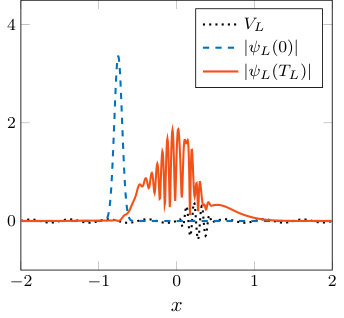 Figure 1
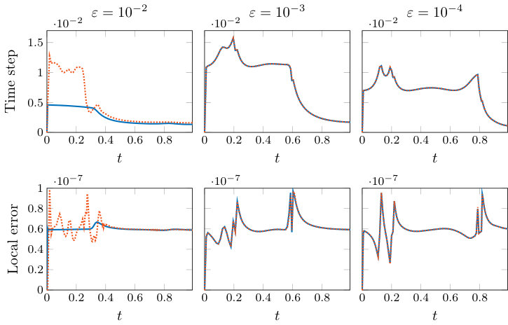 Figure 2
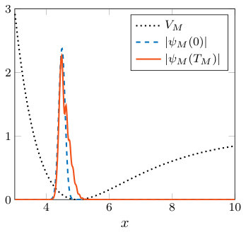 Figure 3
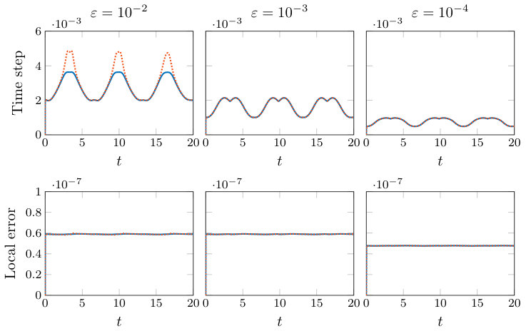 Figure 4
| under lattice potential | under Morse potential | ||||||
| Global | Time | Run | Global | Time | Run | ||
| h | error | steps | time (s) | error | steps | time (s) | |
| adaptive (c) | 490 | 19.5 | 7772 | 320.0 | |||
| adaptive (s) | 394 | 18.7 | 7448 | 316.0 | |||
| smallest (c) | 746 | 11.9 | 10102 | 191.5 | |||
| largest (c) | 217 | 4.1 | 5502 | 104.1 | |||
| 100 | 2.4 | 2000 | 52.0 | ||||
| adaptive (c) | 216 | 12.9 | 13249 | 955.1 | |||
| adaptive (s) | 216 | 14.3 | 13245 | 1021.5 | |||
| smallest (c) | 587 | 14.4 | 19841 | 572.8 | |||
| largest (c) | 64 | 2.9 | 9329 | 315.5 | |||
| 1000 | 20.4 | 20000 | 601.4 | ||||
| adaptive (c) | 215 | 43.7 | 27358 | 12029.7 | |||
| adaptive (s) | 215 | 42.6 | 27343 | 14237.4 | |||
| smallest (c) | 925 | 80.2 | 42555 | 11380.8 | |||
| largest (c) | 90 | 12.0 | 21307 | 6435.6 | |||
| 10000 | 659.8 | 200000 | 60755.0 | ||||
Peer Reviews
No public reviews on file for this paper yet. If you reviewed it on a platform where reviews are public (OpenReview, ICLR, NeurIPS, ICML), you can paste yours below so the community can read it here.
Videos
No videos yet. Explain this paper in a talk, walkthrough, or lecture? Add one.
Time adaptive Zassenhaus splittings
for the Schrödinger equation in the semiclassical regime111This work was supported in part by the Vienna Science and Technology Fund (WWTF) under grant MA14-002. The work of Karolina Kropielnicka on this project was financed by The National Center for Science, under grant no. 2016/23/D/ST1/02061.
Winfried Auzinger
Technische Universität Wien, Institut für Analysis und Scientific Computing, Wiedner Hauptstrasse 8–10/E101, A-1040 Wien, Austria
Harald Hofstätter
Universität Wien, Institut für Mathematik, Oskar-Morgenstern-Platz 1, A-1090 Wien, Austria
Othmar Koch
Universität Wien, Institut für Mathematik, Oskar-Morgenstern-Platz 1, A-1090 Wien, Austria
Karolina Kropielnicka
Institute of Mathematics, University of Gdansk, ul. Wit Stwosz 57, 80-308 Gdansk
Pranav Singh
Mathematical Institute, University of Oxford, Andrew Wiles Building, Radcliffe Observatory Quarter, Woodstock Road, Oxford OX2 6GG
Abstract
Time dependent Schrödinger equations with conservative force field commonly constitute a major challenge in the numerical approximation, especially when they are analysed in the semiclassical regime. Extremely high oscillations originate from the semiclassical parameter, and call for appropriate methods. We propose to employ a combination of asymptotic Zassenhaus splitting with time adaptivity. While the former turns the disadvantage of the semiclassical parameter into an advantage, leading to highly efficient methods with low error constants, the latter enables to choose an optimal time step and to speed up the calculations when the oscillations subside. We support the results with numerical examples.
keywords:
Numerical time integration , time adaptivity , splitting schemes , asymptotic splittings
MSC:
[2010] 65L05 , 65L70 , 81-08
††journal: Appl. Math. Comput.
url]http://www.asc.tuwien.ac.at/ winfried
url]http://www.harald-hofstaetter.at
url]https://mat.ug.edu.pl/ kmalina
url]https://www.maths.ox.ac.uk/people/pranav.singh
1 Introduction
In this paper we are concerned with developing a time-adaptive method for solving the Schrödinger equation in the semiclassical regime,
[TABLE]
with periodic boundary conditions imposed on the interval . The interaction potential is a real and periodic function. The regularity required of and depends on the desired order of the numerical method. For the sake of simplicity, we assume and , where the subscript “” denotes periodicity.
The semiclassical parameter induces oscillations of wavelength in the solution , both in space and in time [1, 2, 3]. In this regime, finite difference schemes require an excessively fine spatial grid and very small time steps [4]. Consequently, they are found to be ineffective in comparison with spectral discretisation in space followed by exponential splittings for time-propagation [1]. Methods based on Lanczos iterations [5], which are particularly effective for problems in the atomic scaling (), are also found to be ineffective in the semiclassical regime, where the exponent involved is of huge spectral size, scaling as , see [6, 7]. Effective methods for highly oscillatory problems, which have a Hamiltonian structure and are periodic in time, have been proposed in [8] and are referred to as Hamiltonian boundary value methods. They have been applied in the context of Schrödinger equations in [9].
In this regime the symmetric Zassenhaus splittings of [10] are found to be very effective. These are asymptotic exponential splittings where exponents scale with powers of the small parameter and, consequently, become progressively small. The small size of these exponents allows a very effective approximation via Lanczos iterations despite reasonably large time steps [10].
Needless to say, the oscillations in the solution change in time. Higher oscillations require smaller time steps, which increases the computational cost. Thus, we face the usual tradeoff between two competing concerns – smaller time steps for higher accuracy and larger time steps for lower cost. Time adaptivity has been a well developed approach to arrive at the optimal compromise by keeping the time steps as large as possible, so long as a prescribed error tolerance is not exceeded. State-of-the-art step-size choice is based on firm theoretical ground by recent investigations of digital filters from signal processing and control theory [11, 12, 13], which have also been demonstrated to enhance computational stability [14]. The advantages of adaptive selection of the time steps in the context of splitting methods have been demonstrated for nonlinear Schrödinger equations in [15], and for parabolic equations in [16]. It is found that in addition to a potential increase in the computational efficiency, the reliability of the computations is enhanced. In an adaptive procedure, the step-sizes are not guessed a priori but chosen automatically as mandated by the smoothness of the solution, and the solution accuracy can be guaranteed.
The aim of this paper is thus to design a time-adaptive method for the Schrödinger equation in the semiclassical regime. This is done by utilising the defect based time adaptivity approach of [17, 18] for the symmetric Zassenhaus splittings of [10]. These time adaptivity schemes, which are very effective for classical splittings, turn out to be successful for the asymptotic splittings of [10] as well.
In Section 2 we describe the defect-based time-adaptive approach. In Section 3 we present a variant of the high-order Zassenhaus splittings of [10], which turns out to be more conducive in a time-adaptive approach. The practical algorithm used for the estimation of the local error for this highly efficient method is derived in Section 4. In Section 5 we present numerical experiments which demonstrate the efficacy of the time-adaptive scheme.
2 Defect-based time adaptivity
Time-adaptivity in numerical solutions of ODEs and PDEs involves adjusting time step of a numerical scheme in order to keep the local error in a single step below a specified error tolerance, . The local error in a single step of a one-step integrator with step-size , starting (without loss of generality) from at ,
[TABLE]
where is the numerical evolution operator, is given by
[TABLE]
where
[TABLE]
is the exact solution. Since the exact evolution operator for (1.1),
[TABLE]
and the exact solution are not available, practical time-adaptivity methods rely on accurate a posteriori estimates of the local error, , that can be computed along with the numerical solution. In this manuscript, we will focus on defect-based estimators of the local error, which are of the form
[TABLE]
Here, is a computable defect term, measuring the local quality of the approximation delivered by the numerical solution, . We will consider two different versions of the defect , see Sections 2.1 and 2.2.
Once an estimate of the local error via (2.1) is available, a new step-size can then be chosen as
[TABLE]
where is the local error tolerance and is the local order of the numerical scheme, . The factor of ensures that we are more conservative with the time step, always taking a slightly smaller time step than predicted ( is usually taken to be a small positive number such as ). When the local error estimate in a step exceeds the error tolerance (), the numerical propagation is run again with the smaller step , otherwise the new time step is used for the next step.
2.1 Classical defect-based estimator
We briefly recall the idea underlying (2.1); see for instance [17]. Thinking of the step-size as a continuous variable and denoting it by (somewhat more intuitive), the discrete flow is a well-defined, smooth function of . We call
[TABLE]
the classical defect (operator) associated with , obtained by plugging in the numerical flow into the given evolution equation (1.1) (which is satisfied exactly by its exact flow ). Due to the definition of , the local error enjoys the integral representation
[TABLE]
Evaluation of requires a single evaluation of the defect at , the step-size actually used in the computation of .222How to compute the defect at , for the given step-size used in the computation, in the context of Zassenhaus splitting will be explained in Section 4.
2.2 Symmetrized defect-based estimator
An alternative way of defining the defect was introduced in [18, 19]. It is based on the fact that the exact evolution operator commutes with the Hamiltionian , whence
[TABLE]
with the anti-commutator . This motivates the definition of the symmetrized defect (operator)
[TABLE]
[TABLE]
Now suppose that is symmetric (time-reversible), i.e., it satisfies . Then, its order is necessarily even, and moreover we even have
[TABLE]
see [18, 19]. This means that in the symmetric case the deviation of the local error estimate based on the symmetrized defect is of a better quality, asymptotically for , than that one based on the classical defect.333Note that , , and . Moreover, evaluation of is typically only slightly more expensive compared to , see [18, 19] for the case of conventional splittings and, in particular, Section 4 below.
3 Symmetric Zassenhaus splittings
Symmetric Zassenhaus splittings are asymptotic splittings introduced in [10] for solving the Schrödinger equation in the semiclassical regime (1.1). These splittings are derived by working in infinite dimensional space, prior to spatial discretisation, which enables a more effective exploitation of commutators, since some of them vanish, while the rest end up being much smaller (in a sense of spectral radius) than generically expected.
To manage the wavelength oscillations in space and time, which arise due to the presence of the small semiclassical parameter , the following relations have been established to be useful for the spatio-temporal resolution in these schemes.
[TABLE]
The Zassenhaus splitting that we will consider in this paper is
[TABLE]
Here,
[TABLE]
are the symmetrized differential operators which first appeared in [10] and have been studied in detail in [20, 3]. These operators are used for preservation of stability under discretization after simplification of commutators.
Once a differential operator such as is discretised to a symmetric differentiation matrix via spectral collocation, its spectral size grows as decreases, since
[TABLE]
Keeping eventual discretisation with the scaling (3.1) in mind, we use a shorthand for the undiscretised and unbounded operator as well. The symmetrized differential operator discretises to the form
[TABLE]
where is a diagonal matrix with values of at the grid points. Its spectral radius grows as , assuming that is independent of , and we abuse notations once more to say , for short.
The splitting (3.2a) possesses several favorable features. First of all, the critical quantities like time step , spatial step and semiclassical parameter are tied together by relation (3.1). As a consequence, the splitting error is expressed via a universal quantity , and the error constant does not hide any critical quantities.
The exponentials involved in the splitting are easily computable after spatial discretization. For example, spectral collocation transforms into a symmetric circulant matrix, whence its exponential may be computed by the Fast Fourier Transform. The diagonal matrix can be exponentiated directly. Neither nor are structured favourably, however their spectral radius is small enough to exponentiate them with a small number (say, 3 or 4) of Lanczos iterations.
Remark 1
Since the splitting (3.2a) which features an error of could loosely be considered a sixth-order splitting with an error constant scaling as . This interpretation is not strictly correct, however, since the error estimate holds for and . For a finite and (i.e. ), the asymptotic Zassenhaus splitting (3.2a) is a highly efficient fourth-order method with a very small error constant. This disparity in the different asymptotic limits occurs because the derivation of (3.2a) involves discarding terms of size , for instance. These terms are under the asymptotic scaling (3.1), , but are under a fixed and . The consequence for the time-adaptivity algorithm (2.1) is that we must use , not .
Remark 2
Many different variants of this splitting are possible (including, but not limited to the case when we start with ). Application of these variants can just as easily be considered, however will not be the focus of the present paper.
Remark 3
The exponents (3.2b) differ from the splitting described in [10] in one minor aspect – the term has been moved from to . This term is of size , which is smaller than and thus may also be combined with . In [10] this term is combined with working under the assumption (time steps larger than ) since is also smaller than under . Consequently, all exponents feature a single power of . This change makes no difference to the overall order of the scheme but makes the computation of defect easier.
4 Local error estimator for Zassenhaus splitting
Remark 4
In the sequel, the argument or , respectively, is suppressed whenever the meaning is obvious.
4.1 Time derivative of the discrete evolution operator
The time-adaptivity algorithm is based on the estimation of the local error in each step, which in turn requires the computation of the defect at discrete time , see Section 2. This requires the computation of For splitting schemes such as (3.2a), this boils down to an application of the product rule, involving computation of the time derivative of each individual exponential.
For exponentials such as
[TABLE]
Now, consider the (modified) Zassenhaus splitting (3.2a) & (3.2b) for (1.1), with the discrete evolution operator re-written in the form
[TABLE]
where , , and
[TABLE]
The derivative of the flow for a splitting scheme can be expressed via the product rule,
[TABLE]
Here the underlined exponentials are the ones that need to be computed freshly. The rest can be dealt with by storing intermediate values from evaluation of the splitting scheme: In order to compute , we store
[TABLE]
which are anyway computed during evaluation of the numerical scheme. In addition, we compute and store
[TABLE]
Then,
[TABLE]
Thus, we need to compute six exponentials appearing in (4.5) in addition to the seven exponentials required in the Zassenhaus splitting (3.2a). For a scheme of order six, we need a total of 13 exponentials.
Remark 5
For the order four method
[TABLE]
five exponentials are required for the Zassenhaus splitting and we have verified that four additional exponentials are required for time adaptivity, making for a total of nine exponentials.
Remark 6
In a practical, memory-efficient implementation, the are computed ‘on the fly’ along with the , via alternating updates of arrays and .
Remark 7
In the above computations, the only feature specific to the Zassenhaus splitting is the use of (4.1b) for the derivative of the exponential. Thus the derivation and the combination of exponentials works in an analogous way for other splittings, with different time derivatives.
4.2 Practical evaluation of the classical defect (2.2)
We need to compute the classical defect at discrete time ,
[TABLE]
Here, , is the Hamiltonian, and is the time derivative according to Section 4.1, see (4.5).
In addition, a small amount of work can be saved by exploiting the relation (see 4.4). Then, computation of amounts to the evaluation of
[TABLE]
4.3 Practical evaluation of the symmetrized defect (2.4)
Instead of (4.6), we need to compute
[TABLE]
With (4.5), we have (again making use of )
[TABLE]
Here the underlined exponential is the one that needs to be computed in addition, compared to evaluation of . Of course, this additional effort is marginal.
Thus, computation of the symmetrized defect at discrete time amounts to evaluation of
[TABLE]
5 Numerical experiments
For our numerical experiments, we will use the wave-packets
[TABLE]
as initial conditions for two experiments. Here
[TABLE]
is a wave-packet with a spread of , mean position and mean momentum . We will consider the evolution of as it heads towards the lattice potential and the evolution of as it oscillates in the Morse potential , which are given by
[TABLE]
respectively, where
[TABLE]
is a bump function.
We consider the behaviour at the final time for the first experiment and for the second experiment under the choices of and . The spatial domain is chosen as for the lattice potential and for the Morse potential, and we impose periodic boundary conditions. The evolution of these wavepackets under the choice is shown in Fig. 1.
As one can observe in Figures 2 and 3, the procedure quickly adapts the time step to ensure that the local accuracy is within the specified threshold, which is taken to be here.
In the first experiment, we use and equispaced points for spatial discretization in the cases and , respectively, while and are used for the three choices of in the second experiment.
In Table 1, we show the total number of time steps required for maintaining the local accuracy of for three cases: and . Also presented are the global accuracies of these solutions at the final time ( and ) and the computational time. These are compared to the (non-adaptive) case when the time step is fixed at (i) the finest value used by the adaptive method (ii) the coarsest value used by the adaptive method (iii) . The reference solutions for computing global errors are produced by using Matlab’s expm function, while using a much finer spatial grid. The number of Lanczos iterations are chosen automatically to meet the accuracy requirements using the a priori error bounds of [21].
We find that for small , the asymptotic scaling yields the smallest error, but the computational effort is prohibitive. The symmetrized error estimate invariantly generates coarser time grids than the classical version, but the additional computational effort implies that the picture is ambivalent in that the computational effort is smaller in only about half of the cases. When the largest step generated by the adaptive strategy ‘(c)’ is used in a uniform grid, computations are fast but not sufficiently accurate, while use of the smallest adaptive time step is prohibitively expensive in the case of the lattice potential (for the Morse potential, the reduction in the number of time steps is outweighed by the computational effort for the error estimate). Together, these two observations imply that adaptive step-size choice constitutes the appropriate means to determine grids that reproduce the solution in a reliable and efficient way, and excels over a priori choice of the step-size. In particular, the guess of an optimal step-size is commonly not feasible, while the adaptive strategy finds the time steps automatically and guarantees the desired level of accuracy.
6 Conclusions
We have investigated adaptive strategies used in conjunction with asymptotic Zassenhaus splitting for the solution of linear time-dependent Schrödinger equations in the semiclassical regime. The local time-stepping is based on defect-based error estimation strategies. We have demonstrated that adaptivity provides a means to reliably and efficiently achieve a desired level of accuracy especially for a small semiclassical parameter and thus excels over fixed time steps in many cases. A major benefit is in addition that no near-optimal equidistant step-size has to be guessed a priori.
The reference list from the paper itself. Each links out to its DOI / PubMed record.
- 1[1] W. Bao, S. Jin, P. A. Markowich, On time-splitting spectral approximations for the Schrödinger equation in the semiclassical regime, J. Comput. Phys. 175 (2002) 487–524. doi:10.1006/jcph.2001.6956 . · doi ↗
- 2[2] S. Jin, P. Markowich, C. Sparber, Mathematical and computational methods for semiclassical Schrödinger equations, Acta Numerica 20 (2011) 121–210.
- 3[3] P. Singh, High accuracy computational methods for the semiclassical Schrödinger equation, Ph.D. thesis, University of Cambridge (2017).
- 4[4] P. A. Markowich, P. Pietra, C. Pohl, Numerical approximation of quadratic observables of Schrödinger-type equations in the semi-classical limit, Numer. Math. 81 (4) (1999) 595–630.
- 5[5] Y. Saad, Analysis of some Krylov subspace approximations to the matrix exponential operator, SIAM J. Numer. Anal. 29 (1) (1992) 209–228.
- 6[6] M. Hochbruck, C. Lubich, On Krylov subspace approximations to the matrix exponential operator, SIAM J. Numer. Anal. 34 (1997) 1911–1925.
- 7[7] C. Lubich, From Quantum to Classical Molecular Dynamics: Reduced Models and Numerical Analysis, Zurich Lectures in Advanced Mathematics, European Mathematical Society, Zurich, 2008.
- 8[8] L. Brugnano, J. Montijano, L. Randez, On the effectiveness of spectral methods for the numerical solution of multi-frequency highly oscillatory Hamiltonian problems, Numer. Algorithms 81 (2019) 345––376.