Unpriortized Autoencoder For Image Generation
Jaeyoung Yoo, Hojun Lee, Nojun Kwak

TL;DR
This paper introduces a novel autoencoder-based image generation method that explicitly estimates the latent distribution using a latent density estimator, resulting in improved image quality over previous models.
Contribution
It proposes a new approach to image generation with autoencoders by directly estimating the latent distribution, bypassing manual prior assumptions.
Findings
Generated images have higher visual quality.
The model outperforms previous autoencoder-based generative models.
Explicit latent distribution estimation improves generation results.
Abstract
In this paper, we treat the image generation task using an autoencoder, a representative latent model. Unlike many studies regularizing the latent variable's distribution by assuming a manually specified prior, we approach the image generation task using an autoencoder by directly estimating the latent distribution. To this end, we introduce 'latent density estimator' which captures latent distribution explicitly and propose its structure. Through experiments, we show that our generative model generates images with the improved visual quality compared to previous autoencoder-based generative models.
Click any figure to enlarge with its caption.
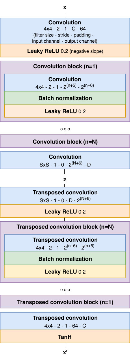 Figure 1
 Figure 2
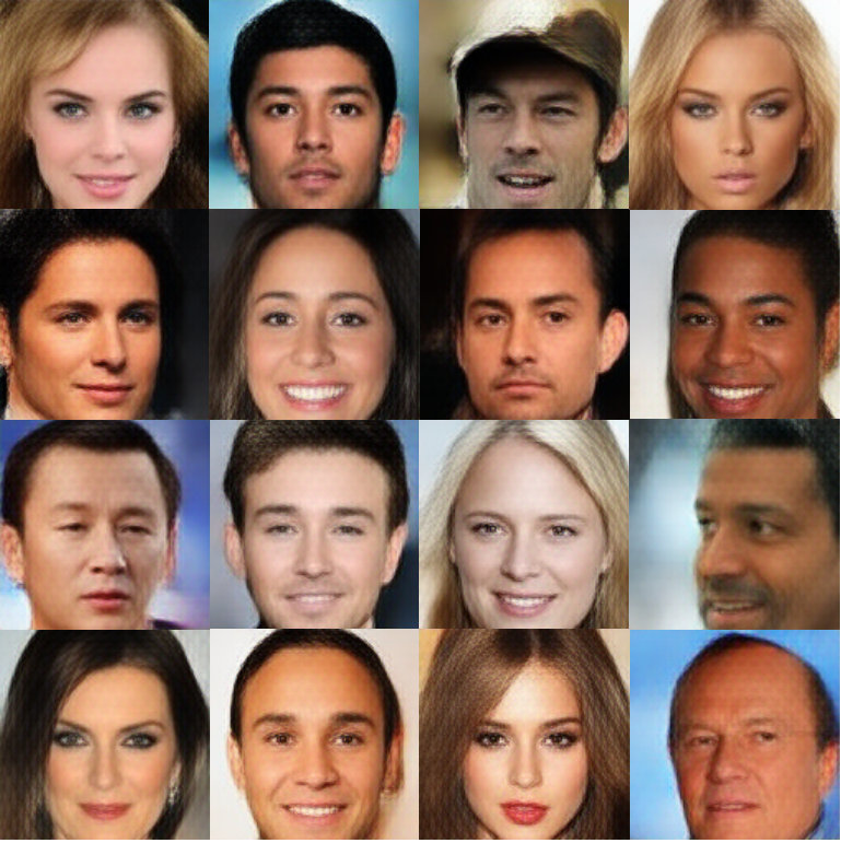 Figure 1
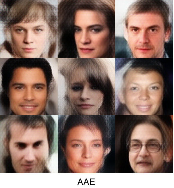 Figure 4
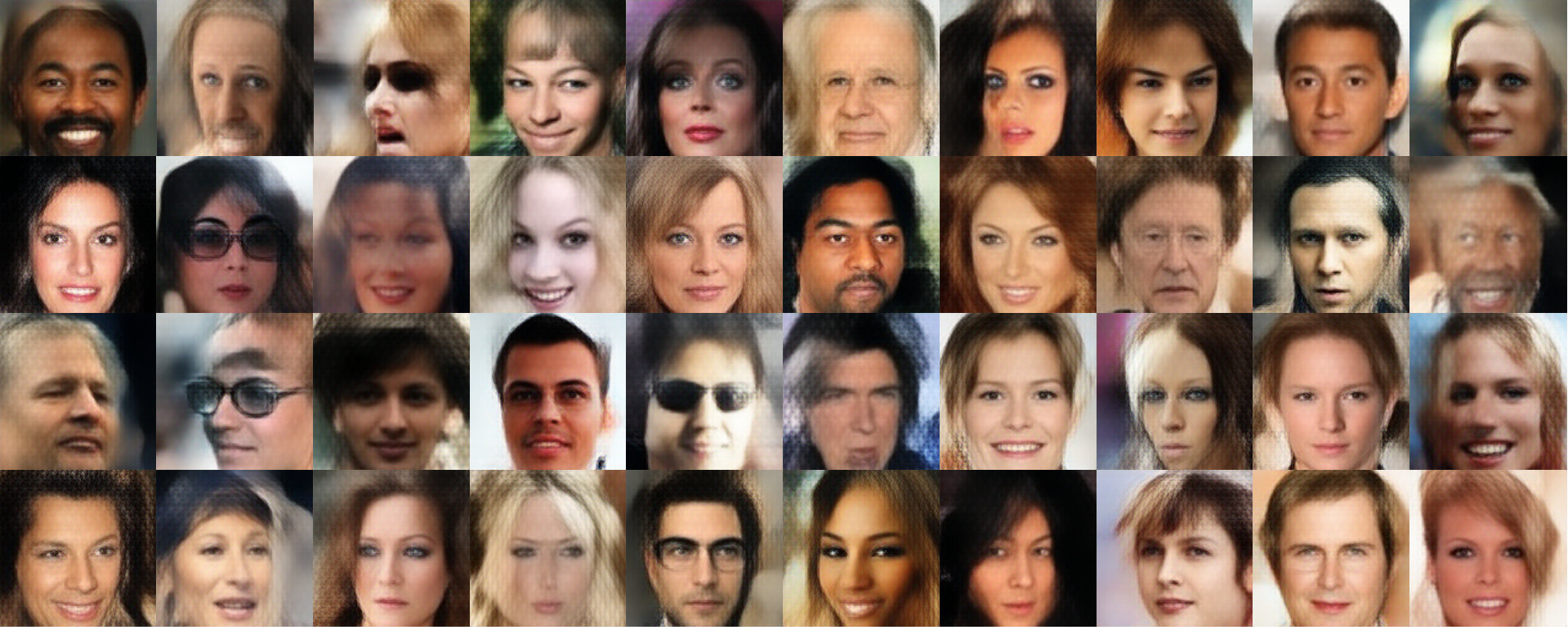 Figure 5
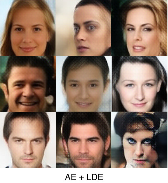 Figure 6
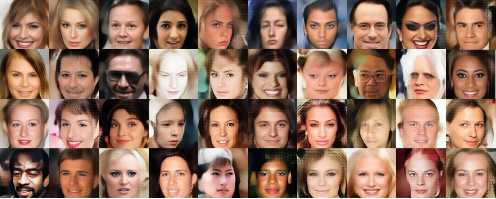 Figure 7
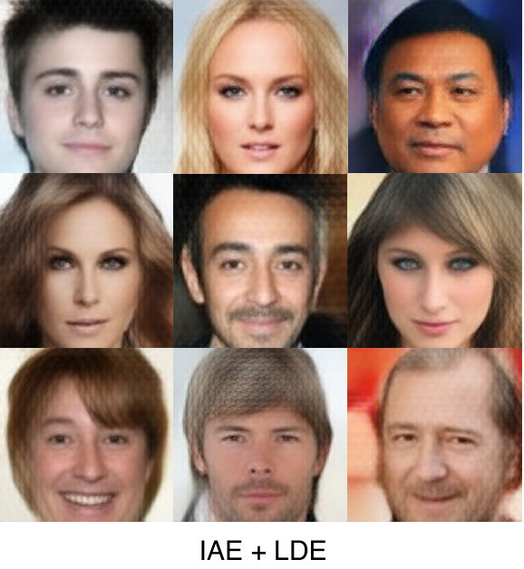 Figure 8
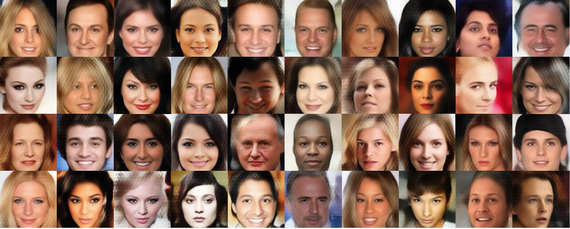 Figure 9
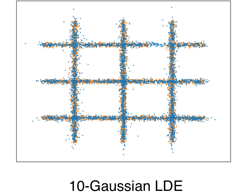 Figure 10
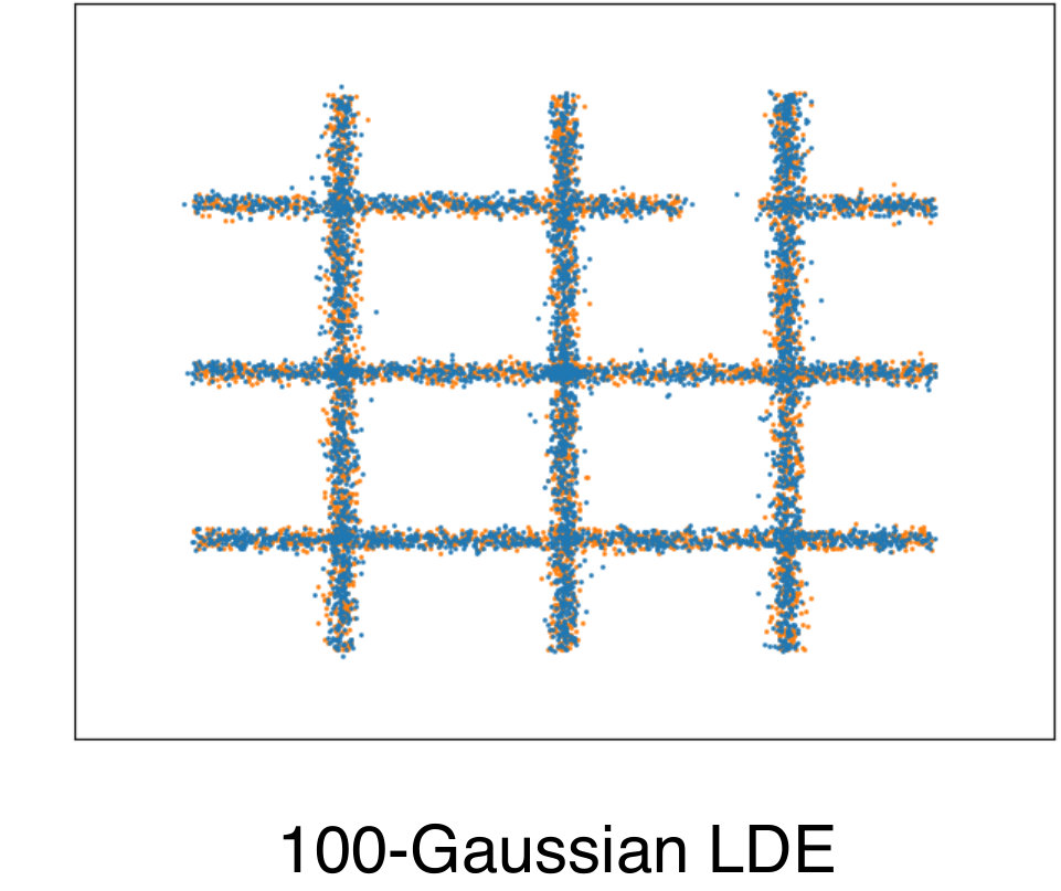 Figure 11
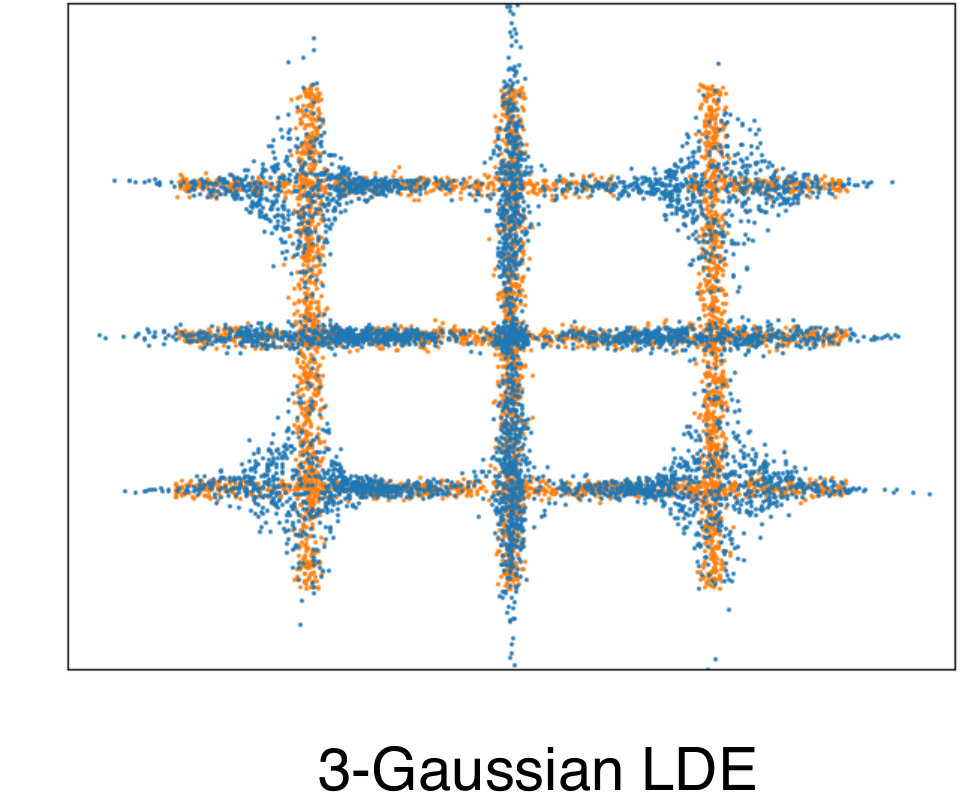 Figure 12
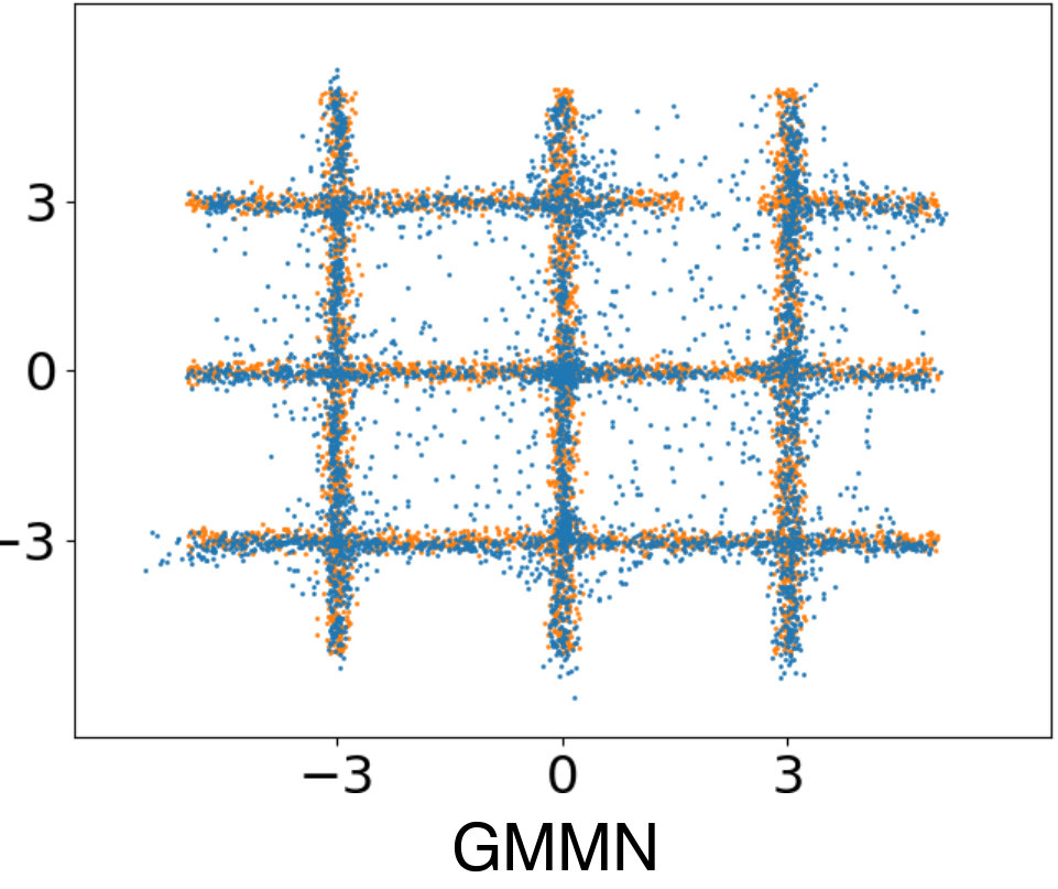 Figure 13
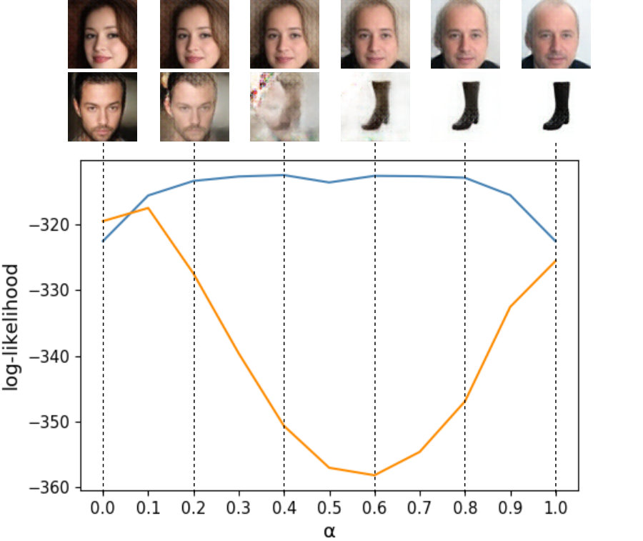 Figure 14
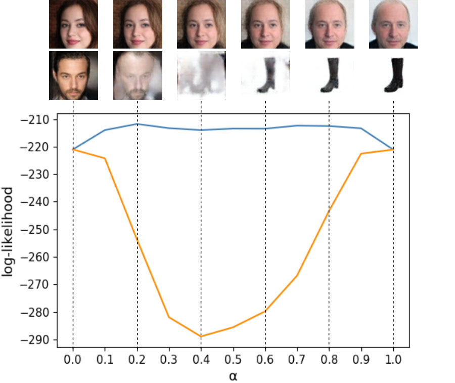 Figure 15
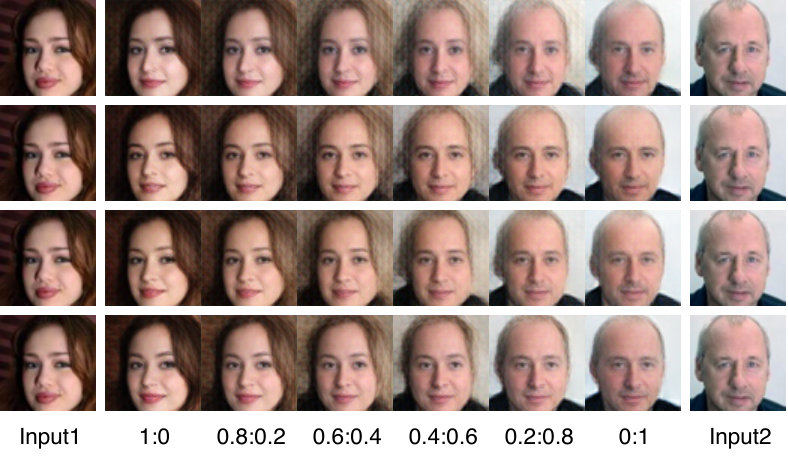 Figure 16
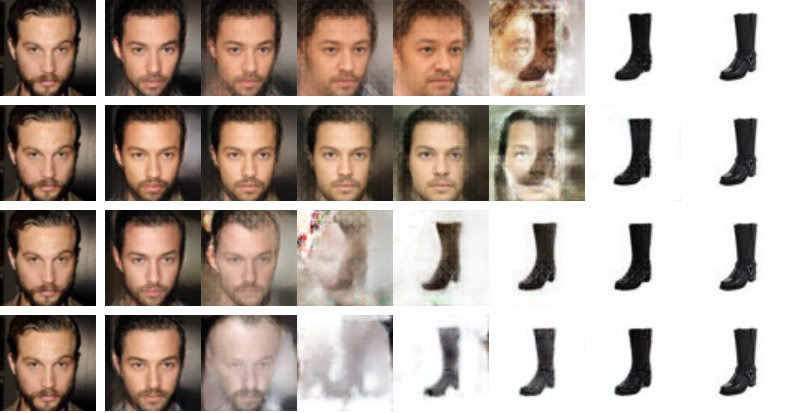 Figure 17
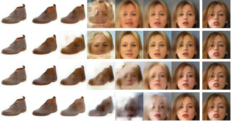 Figure 18
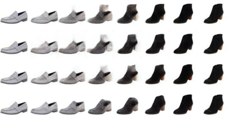 Figure 19
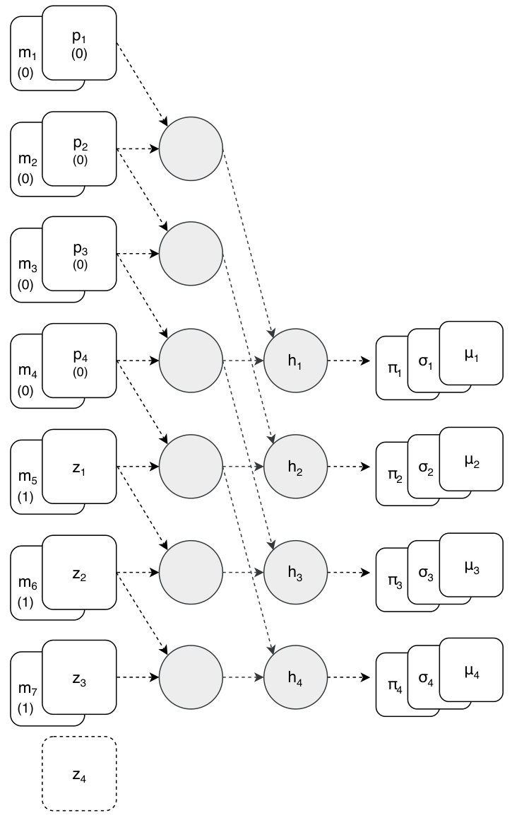 Figure 20
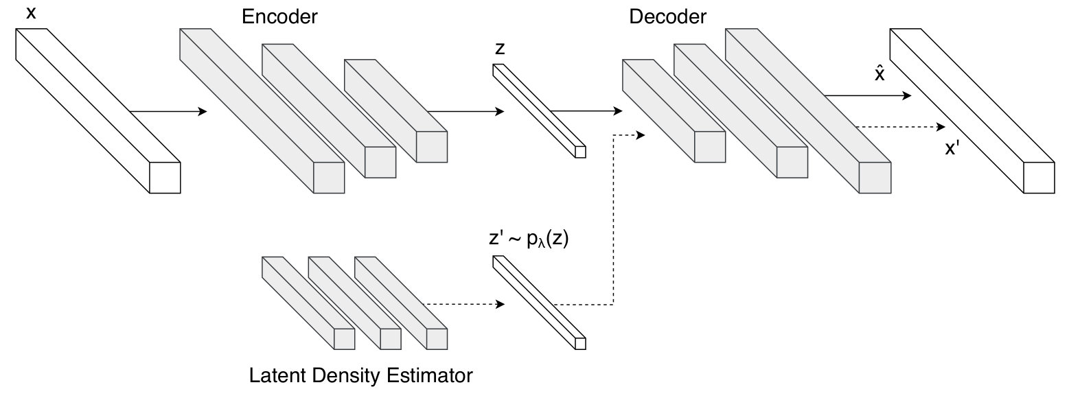 Figure 21
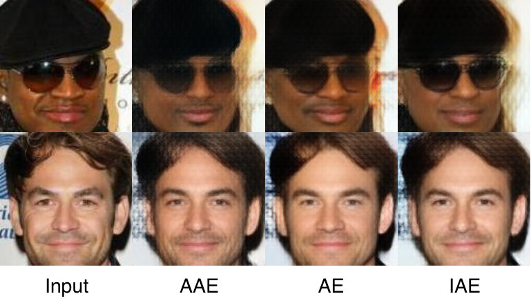 Figure 22
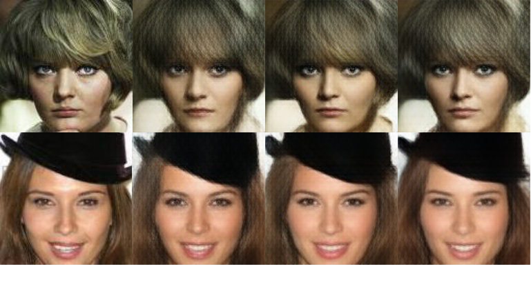 Figure 23
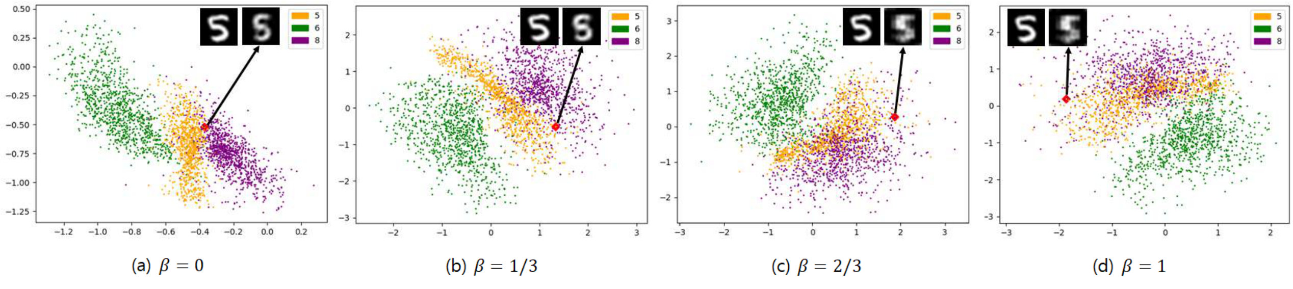 Figure 24
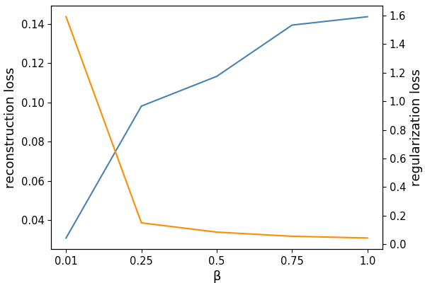 Figure 25
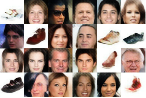 Figure 26
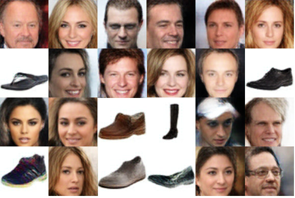 Figure 27
Peer Reviews
No public reviews on file for this paper yet. If you reviewed it on a platform where reviews are public (OpenReview, ICLR, NeurIPS, ICML), you can paste yours below so the community can read it here.
Videos
No videos yet. Explain this paper in a talk, walkthrough, or lecture? Add one.
Taxonomy
MethodsSolana Customer Service Number +1-833-534-1729
Unpriortized Autoencoder for Image Generation
Abstract
In this paper, we treat the image generation task using an autoencoder, a representative latent model. Unlike many studies regularizing the latent variable’s distribution by assuming a manually specified prior, we approach the image generation task using an autoencoder by directly estimating the latent distribution. To this end, we introduce ‘latent density estimator’ which captures latent distribution explicitly and propose its structure. Through experiments, we show that our generative model generates images with the improved visual quality compared to previous autoencoder-based generative models.
**Index Terms— ** Autoencoder, Image Generation, Generative Model, Density Estimation, Mixture Model
1 Introduction
Data generation using an autoencoder is performed by sampling from the latent distribution which is the distribution of the latent variables. Therefore, how to express the latent distribution and how to sample a latent variable is a core problem in the task of extending an autoencoder to a generative model.
Most existing studies, such as variational autoencoder (VAE) [1], approach this problem by assuming a prior as a manually specified distribution (e.g. fully factorized Gaussian). However, manually specified prior may differ from the complex latent nature of the actual data. This difference makes a trade-off between reconstruction and prioritized regularization. In the Figure 2, we can see that the reconstructed digits are blurry as the weight of the regularization term increases. As a result, it adversely affects the reconstruction and makes a difference between the real latent distribution and the prior, which leads to degradation of the generation quality.
As another approach, we can think of extending autoencoders to generative models by estimating latent distribution from the data. This method is free from the above-mentioned trade-off between the reconstruction and the regularization because the autoencoder can be trained without extra regularization term of the latent distribution. However, in this approach, returning to the nature of the latent variable and the prior, we need to consider a couple of things: (1) The distribution of learned latent variables without prioritized regularization can have a complex form. Therefore, we should be able to model this distribution flexibly. (2) An autoencoder trained solely from data points may be over-fitted or does not learn a proper manifold. The autoencoder should be able to learn meaningful representation via latent variables.
In this paper, we extend the autoencoder to the generative models by estimating the empirical distribution of latent variables obtained from a given dataset using an additional network named as the Latent Density Estimator (LDE). The proposed LDE learns complex distributions flexibly using an auto-regressive approach. Also, in order to preferentially learn the important representation of the given data through the latent variables, we exploit a training strategy that incrementally increases the effective size of the latent vector. As shown in Figure 1, our method generates clear and diverse images that reflect the characteristics of data well.
2 Related Works
A typical study, variational autoencoder (VAE) [1], performs regularization to minimize the KL divergence between the distribution of latent variables and the assumed prior by maximizing the evidence lower bound (ELBO). Another study, adversarial autoencoder (AAE) [2], uses adversarial training. The encoder is considered as a generator of the latent variables and it is learned to imitate the prior distribution, which acts as a regularization for the latent distribution.
These studies have a drawback in that they must assume a prior in advance of training and must force the latent distribution into a specific form. Normalizing flow [3] approaches this problem by allowing a more flexible latent distribution to be applied to posterior sequences of invertible transformations. And there are various studies that modified or extended the normalizing flow [4, 5, 6, 7].
Unlike previous studies, the latent density estimator (LDE) learns the prior by estimating an explicit form of the probability density of the latent variables . In our method, the latent vector is sampled from a latent distribution estimated by LDE.
3 Latent Density Estimation
3.1 Problem formulation
An autoencoder consists of an encoder and a decoder, which encodes a data point into a latent vector () and reconstructs from (), respectively. Ideally, if a latent vector can be sampled from a true distribution of , it is possible to generate data using the decoder
Our goal is to directly estimate the latent distribution which represents the dataset well. We deal with this problem by estimating the probability density function of from dataset using a additional density estimator parameterized by . The density estimator is trained to find that maximizes the likelihood of for as follows.
[TABLE]
Here, the is the empirical latent distribution obtained from and the encoder and the LDE estimates by .
3.2 Overview of the proposed method
Figure 3 shows the overall structure of the proposed method for extending autoencoder into generative models. As can be seen in the figure, the architecture of the proposed generative framework consists of an encoder, a decoder and a latent density estimator (LDE).
The encoder and the decoder are used in the form of the deterministic function. The LDE expresses the probability density function of explicitly. In the generation process, a latent vector is randomly sampled from and generates new data through the decoder.
In this framework, the autoencoder and the LDE are trained according to the following training procedure. First, we train the autoencoder to reconstruct . Second, after the completion of training the autoencoder, we obtain from using the encoder . Finally, we train the latent density estimator to estimate using .
3.3 Latent Density Estimator (LDE)
The proposed approach of LDE is based on the method in RNADE [8]. If is a -dimimensional real-valued vector whose -th element is denoted by , we factorize using the chain rule:
[TABLE]
Here, is . The estimated probability density of the -th variable of is conditionally calculated by the values of the variables with lower indices as . It is calculated as follows by the mixture of univariate Gaussian with its parameters being the mixing coefficient , the mean and the standard deviation :
[TABLE]
Here, the parameters , and are estimated by the LDE. The LDE is learned to find , and by minimizing the loss function which is calculated as the average of all the negative log of (3), :
[TABLE]
As shown in Figure 4, the LDE network consists of two parts: dilated causal convolution [9] and Mixture Density Network [10]. The dilated causal convolution outputs a series of causal features using . Each observes . The zero vector is to match the dimension of the input to the first output to , and is used to distinguish from by setting the masking value as 1 and 0, respectively. The Mixture Density Network estimates the parameters of the mixture of Gaussians, , and , from using an convolution layer. Here, and are obtained by the linear and the exponential activations, respectively, and is the softmax output for the Gaussians.
3.4 Incremental learning of latent vector
Instead of adding an regularization term to the objective function, we use the structural characteristics of an autoencoder to make an autoencoder learn salient factors of data. In the training process, initially only a small part of the latent vector is used to learn the autoencoder. Then, as the iteration goes on, the effective size of the latent vector is increased gradually. Here, the unused part of the latent vector is masked to zero. This incremental learning strategy of the latent variables induces the autoencoder to learn the most important representation of data first.
3.5 Objective Function
For the training of the autoencoder, we use the distance in the pixel space and the perceptual loss [11] as follows:
[TABLE]
where is the mean sqaured error in the pixel space, is perceptual loss as in [11] and is the weight parameter for the perceptual loss.
4 Experiments
We will call the autoencoder whose latent vector is trained by applying the incremental learning as IAE. And, AE will denote an autoencoder trained without the incremental learning. For fair comparison, the autoencoders of AAE and ours use the same structure. We use (5) as the reconstruction loss of AAE and ours with the of 0.1. The perceptual loss was calculated using the feature maps at relu11, relu21, and relu31 of Imagenet [12] pretrained VGG19 [13]
4.1 Log-likelihood of the Latent Density Estimator
To quantitatively compare the density estimation performance of the LDE, we measured the log-likelihood in natural images according to the experimental setup of [8, 14]. We perform the same preprocessing of [8, 14] in the BSDS300[16] dataset. Table 1 shows the log-likelihoods of various density estimators. In this experiment, when is 10 and 30, the results of our method, LDE, not only outperformed mixture of Gaussian based methods, but also show the best score against all other density estimator compared. In our results, too simple model, LDE with =1, shows the worst performance, and when the model is complex, LDE with =100, the performance becomes lower than that of LDE with =30.
4.2 Latent Space Walking on Two Domains
In order to understand the representation and structure of the latent space, we perform linearly interpolating two latent vectors. We trained the AAE with a Gaussian prior (), the AAE with a mixture of two Gaussian prior ( and ), AE and IAE that use an 100-dimensional latent vector using the Shoes[17] and CelebA[18] datasets with a size of . Figure 5 shows the results obtained by linearly interpolating two test samples in the latent space for three cases. Figure 5 (a) shows the interpolation on the CelebA and (b) shows the results on the Shoes datasets, both of which are the interpolation in the same domain. Every results of (a) are generally plausible, it shows that the face attributes such as visual age change smoothly. However, in (b), only the results of IAE change the shape continuously. Figure 5 (c) shows the interpolation between different data domains. AAE produces an image in which a person’s face and shoes are overlapped during interpolation. In contrast to AAE, our IAE produces images that can not be seen as shoes or human faces in the middle. In fact, the images of a person’s face and those of shoes belong to the semantically different data domain from each other, so this gaps can be meaningful for the latent representation of an autoencoder.
4.3 Image Generation
For qualitative comparison of generation results, We performed image generation on CelebA. The LDE with 30 mixture of Gaussian was applied to AE and IAE. Figure 6 shows 6 random generation results for AAE, AE with LDE, and IAE with LDE. For a fair comparison, we present successively generated samples, not cherry picking the samples. As with the image quality, the generation results of AAE are generally unclear. AE with LDE produces the more sharp and detailed image compared to AAE, but failure cases are often generated. The results of IAE with LDE show the most stable and best image quality among the compared methods.
4.4 Log-likelihood of Generative Models
When the log-likelihood can not be computed directly, the Parzen window based density estimation is a commonly used method for evaluation of generative models. We used this evaluation method as specified in [19, 21, 2]. We trained our generative models without perceptual loss. The dimensionality of the latent vector used was 8 for MNIST[23] and 15 for TFD[24]. of LDE is 30 and the scale parameters of the Gaussian kernel are found through the grid search on the validation set. As can be seen in the table 2, our results show the lower likelihood compared to AAE and eVAE on MNIST, but we achieved the highest log-likelihood far beyond the previous methods on TFDs, relatively a more complex dataset than MNIST.
5 Conclusion
In this paper, we tackle the autoencoder-based image generation task without using regularization by a specified prior. We introduced the latent density estimator to estimate the latent distribution. In addition, we proposed an incremental learning strategy of latent vector so that the autoencoder can learn a meaningful representation. The proposed LDE showed better performance than the previous studies in density estimation. As a result, the autoencoder applying the latent density estimator improves the generation quality of the autoencoder based generative models.
The reference list from the paper itself. Each links out to its DOI / PubMed record.
- 1[1] Diederik P Kingma and Max Welling, “Auto-encoding variational bayes,” ar Xiv preprint ar Xiv:1312.6114 , 2013.
- 2[2] Alireza Makhzani, Jonathon Shlens, Navdeep Jaitly, Ian Goodfellow, and Brendan Frey, “Adversarial autoencoders,” ar Xiv preprint ar Xiv:1511.05644 , 2015.
- 3[3] Danilo Rezende and Shakir Mohamed, “Variational inference with normalizing flows,” in International Conference on Machine Learning , 2015, pp. 1530–1538.
- 4[4] Diederik P Kingma, Tim Salimans, Rafal Jozefowicz, Xi Chen, Ilya Sutskever, and Max Welling, “Improved variational inference with inverse autoregressive flow,” in Advances in Neural Information Processing Systems , 2016, pp. 4743–4751.
- 5[5] George Papamakarios, Iain Murray, and Theo Pavlakou, “Masked autoregressive flow for density estimation,” in Advances in Neural Information Processing Systems , 2017, pp. 2338–2347.
- 6[6] Chin-Wei Huang, David Krueger, Alexandre Lacoste, and Aaron Courville, “Neural autoregressive flows,” in Proceedings of the 35th International Conference on Machine Learning , Jennifer Dy and Andreas Krause, Eds., Stockholmsmässan, Stockholm Sweden, 10–15 Jul 2018, vol. 80 of Proceedings of Machine Learning Research , pp. 2078–2087, PMLR.
- 7[7] Laurent Dinh, Jascha Sohl-Dickstein, and Samy Bengio, “Density estimation using real nvp,” ar Xiv preprint ar Xiv:1605.08803 , 2016.
- 8[8] Benigno Uria, Iain Murray, and Hugo Larochelle, “Rnade: The real-valued neural autoregressive density-estimator,” in Advances in Neural Information Processing Systems , 2013, pp. 2175–2183.