On the Robust PCA and Weiszfeld's Algorithm
Sebastian Neumayer, Max Nimmer, Simon Setzer, Gabriele Steidl

TL;DR
This paper introduces a robust PCA method based on minimizing Euclidean distances to data points using a Weiszfeld-like algorithm, effectively handling outliers and ensuring convergence to critical points.
Contribution
It develops a novel Weiszfeld-like algorithm for robust PCA that carefully manages anchor directions and proves its global convergence.
Findings
Algorithm demonstrates excellent performance in numerical tests.
Handles anchor directions with careful mathematical treatment.
Proven convergence to critical points under Kurdyka-Łojasiewicz property.
Abstract
Principal component analysis (PCA) is a powerful standard tool for reducing the dimensionality of data. Unfortunately, it is sensitive to outliers so that various robust PCA variants were proposed in the literature. This paper addresses the robust PCA by successively determining the directions of lines having minimal Euclidean distances from the data points. The corresponding energy functional is not differentiable at a finite number of directions which we call anchor directions. We derive a Weiszfeld-like algorithm for minimizing the energy functional which has several advantages over existing algorithms. Special attention is paid to the careful handling of the anchor directions, where we take the relation between local minima and one-sided derivatives of Lipschitz continuous functions on submanifolds of into account. Using ideas for stabilizing the classical Weiszfeld…
Click any figure to enlarge with its caption.
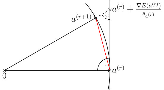 Figure 1
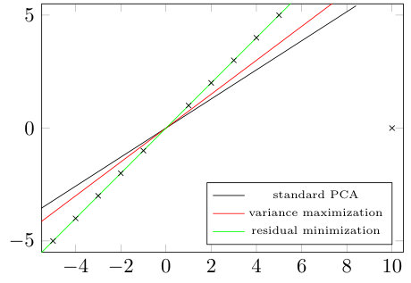 Figure 2
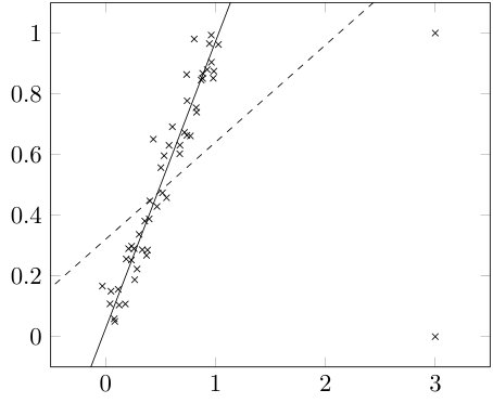 Figure 3
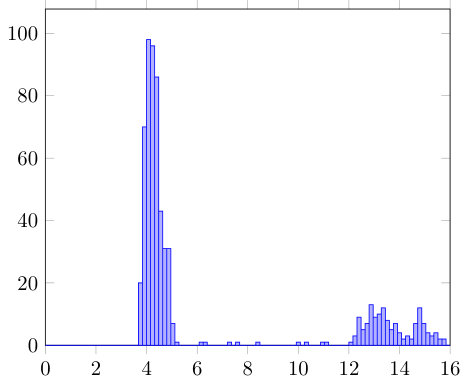 Figure 4
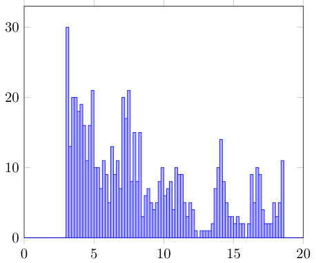 Figure 5
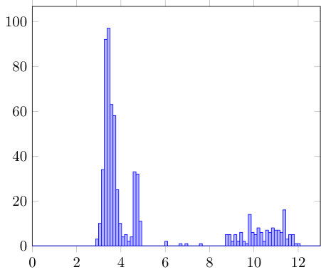 Figure 6
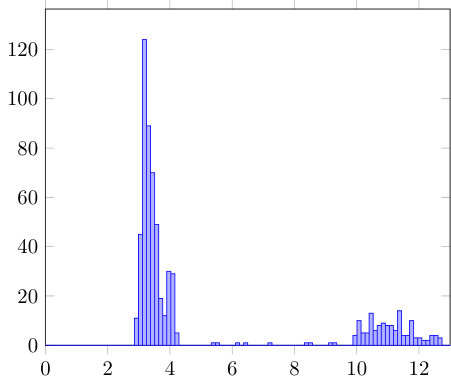 Figure 7
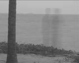 Figure 8
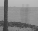 Figure 9
 Figure 10
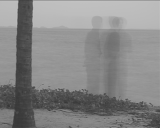 Figure 11
 Figure 12
 Figure 13
 Figure 14
 Figure 15
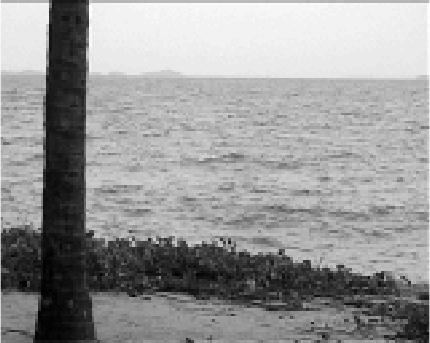 Figure 16
 Figure 17
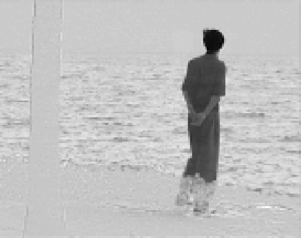 Figure 18
 Figure 19
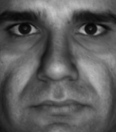 Figure 20
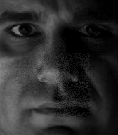 Figure 21
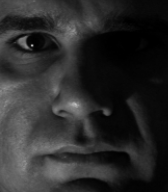 Figure 22
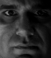 Figure 23
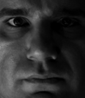 Figure 24
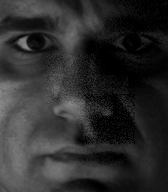 Figure 25
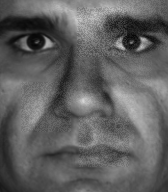 Figure 26
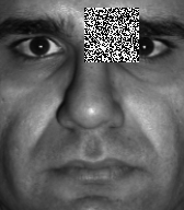 Figure 27
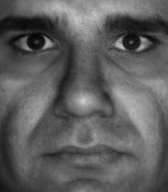 Figure 28
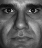 Figure 29
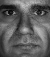 Figure 30
Peer Reviews
No public reviews on file for this paper yet. If you reviewed it on a platform where reviews are public (OpenReview, ICLR, NeurIPS, ICML), you can paste yours below so the community can read it here.
Videos
No videos yet. Explain this paper in a talk, walkthrough, or lecture? Add one.
Taxonomy
TopicsSparse and Compressive Sensing Techniques · Advanced Statistical Methods and Models · Face and Expression Recognition
\setkomafont
sectioning \setkomafonttitle \setkomafontdescriptionlabel
On the Robust PCA and Weiszfeld’s Algorithm
Sebastian Neumayer111Department of Mathematics, Technische Universität Kaiserslautern, Paul-Ehrlich-Str. 31, D-67663 Kaiserslautern, Germany, {nimmer,steidl}@mathematik.uni-kl.de.
Max Nimmer111Department of Mathematics, Technische Universität Kaiserslautern, Paul-Ehrlich-Str. 31, D-67663 Kaiserslautern, Germany, {nimmer,steidl}@mathematik.uni-kl.de.
Simon Setzer333Engineers Gate, London, United Kingdom
Gabriele Steidl111Department of Mathematics, Technische Universität Kaiserslautern, Paul-Ehrlich-Str. 31, D-67663 Kaiserslautern, Germany, {nimmer,steidl}@mathematik.uni-kl.de. 222Fraunhofer ITWM, Fraunhofer-Platz 1, D-67663 Kaiserslautern, Germany
Abstract
The principal component analysis (PCA) is a powerful standard tool for reducing the dimensionality of data. Unfortunately, it is sensitive to outliers so that various robust PCA variants were proposed in the literature. This paper addresses the robust PCA by successively determining the directions of lines having minimal Euclidean distances from the data points. The corresponding energy functional is not differentiable at a finite number of directions which we call anchor directions. We derive a Weiszfeld-like algorithm for minimizing the energy functional which has several advantages over existing algorithms. Special attention is paid to the careful handling of the anchor directions, where we take the relation between local minima and one-sided derivatives of Lipschitz continuous functions on submanifolds of into account. Using ideas for stabilizing the classical Weiszfeld algorithm at anchor points and the Kurdyka–Łojasiewicz property of the energy functional, we prove global convergence of the whole sequence of iterates generated by the algorithm to a critical point of the energy functional. Numerical examples demonstrate the very good performance of our algorithm.
1 Introduction
Principal component analysis (PCA) [41] is an important tool for dimensionality reduction of data which is often applied as a pre-processing step, e.g., for classification or segmentation. The procedure provides dimensionality reduction by projecting the data onto a linear subspace maximizing the variance of the projection or, equivalently minimizing the squared Euclidean distance error to the subspace. More precisely, let data points be given. By we denote the Euclidean norm and by the identity matrix. PCA finds a -dimensional affine subspace , , having smallest squared Euclidean distance from the data:
[TABLE]
While and in the above minimization problem are not unique, the affine subspace itself is uniquely determined if the empirical covariance matrix only has eigenvalues of multiplicity one, and goes through the offset(bias) . Therefore we can reduce our attention to data points , and subspaces through the origin minimizing the squared Euclidean distances to the , . Setting further the gradient of the inner function in (1) with respect to to zero and adding the constraint of being in the Stiefel manifold to eliminate some redundancies the problem reduces to
[TABLE]
where denotes the orthogonal projection onto .
One of the most important properties of PCA is the nestedness of the PCA subspaces, i.e., for , the optimal -dimensional PCA subspace is contained in the -dimensional one. In particular, the directions forming the columns of can be found successively by computing for ,
[TABLE]
or equivalently
[TABLE]
where , , and , see, e.g., [13]. The first problem (3) focuses on the minimization of the residual, while the second one (4) underlines the maximization of the variance in the PCA direction.
Unfortunately, PCA is sensitive to outliers in the data, see Fig. 1. One possibility to circumvent the problem is to remove outliers before computing the principal components. However, in some contexts, outliers are difficult to identify and other data points are incorrectly given outlier status forcing a large number of deletions before a reliable estimate can be found.
Therefore, quite different methods were proposed in the literature to make PCA robust, in particular in robust statistics, see the books [16, 33, 28]. One approach consists in assigning different weights to data points based on their estimated relevance, to get a weighted PCA, see, e.g. [21]. The RANSAC algorithm [9] repeatedly estimates the model parameters from a random subset of the data points until a satisfactory result is obtained as indicated by the number of data points within a certain error threshold. In a similar vein, least trimmed squares PCA models [45, 44] aim to exclude outliers from the squared error functional, but in a deterministic way. Another possible approach is to minimize the median of the squared errors as in [34].
The variational model of Candes et al. [5] decomposes the data matrix into a low rank and a sparse part by minimizing
[TABLE]
exploiting the nuclear norm of and the sum of the absolute values of entries . Then can be considered as robust part, while addresses the outliers. Related approaches as [35, 52] separate the low rank component from the column sparse one using similar norms.
Another group of robust PCA approaches replaces the squared norm in PCA by the norm. Then the minimization of the energy functional can be addressed by linear programming, see, e.g., Ke and Kanade [19]. Unfortunately, this norm is not rotationally invariant.
Mathematically interesting approaches follow (1) - (4), but skip the squares in the Euclidean distances and the inner products to find more robust directions. Taking pure Euclidean distances has several consequences. First of all, the energy functionals become non-differentiable at a finite number of subspaces spanned by matrices , resp. directions , which we collect within the so-called anchor set. Further, the offset in
[TABLE]
cannot be simply determined, see our small discussion in Section 5. Let us assume that an offset is given, so that we can restrict our attention to the data and (5) becomes
[TABLE]
Even then we lose the nested subspace property of the classical PCA, so that in particular
[TABLE]
and
[TABLE]
have in general nothing to do with the columns of the matrix obtained in (6). Finally, the residual minimizing point of view (7) leads to different results than the variance maximizing one in (8), see Fig. 2.
The models (6) - (8) were considered in the literature. The maximization of (8) was suggested with more general scalable functions than just the absolute value by Huber [15, p. 203] and studied in detail as PP-PCA by Li and Chen [29]. It was reinvented and tackled with a greedy algorithm in [25] and the greedy algorithm was made more robust using median computations in [14]. For other methods in this direction, see also [35, 39]. In [14] it was pointed out that the variance maximizing method in [25] lacks a certain robustness since it still involves mean computations. This was already demonstrated in Fig. 2.
Model (6) was treated by Ding et al. [7], where the authors circumvented the anchor set by smoothing the original energy functional. The paper gives no convergence analysis of the proposed algorithm. A tight convex relaxation approach for (6), called REAPER was suggested in [27]. The relaxation replaces the condition that the symmetric positive semidefinite matrix has eigenvalues in by the condition of eigenvalues in . This blows the problem size up. Numerically the relaxed problem can be solved via an iteratively re-weighted least squares algorithm. Usually this requires again a smoothing of the relaxed convex, but still non-differentiable functional.
In this paper, we are interested in the residual minimizing approach (7). Recently, a minimization algorithm was published by Keeling and Kunisch [20]. Local convergence of their algorithm to a local minimizer was proved if the two parameters within the algorithm are chosen appropriately without a concrete specification of their range. The outcome of the algorithm is very sensitive to the choice of the parameters. We propose a minimization algorithm which is completely different from those in [20]. It is based on ideas of the classical Weiszfeld algorithm [51] for computing the geometric median of points in and has the advantage that no parameters have to be tuned. In non-anchor directions the algorithm can be considered as gradient descent algorithm on the sphere, where the length of the gradient descent is automatically given. The treatment of anchor directions relies on one-sided directional derivatives of the energy functional. We show that such derivatives can be used to characterize local minima on submanifolds of of locally Lipschitz continuous functions which is interesting on its own. We prove global convergence of our algorithm to a critical point of the energy functional, where we take special care of the anchor set.
Outline of the paper
In the next Section 2, we recall the Weiszfeld algorithm for computing the geometric median of given data points. Properties of the energy function, critical point conditions and the minimization algorithm are developed in Section 3. The main part of the paper is the convergence analysis of our algorithm in Section 4. Some remarks on the offset are given in Section 5. Numerical examples demonstrate the performance of our algorithm in Section 6. The paper ends with conclusions and ideas for future work in Section 7. The Appendix A provides a criterion for determining local minimizers of locally Lipschitz continuous functions on embedded manifolds in which is applied in Section 3.
2 Weiszfeld’s Algorithm for Geometric Median Computation
We start with a small review of Weiszfeld’s algorithm with two aims: first, the geometric median usually replaces the mean as offset in robust PCA methods. Second, having the original Weiszfeld algorithm in mind helps to understand the basic intention of our algorithm for minimizing (7).
The geometric median of pairwise distinct points , , which are not aligned, is uniquely determined by
[TABLE]
An efficient algorithm for solving the geometric median problem is the Weiszfeld algorithm which goes back to the Hungarian mathematician A. Vazsonyi (Weiszfeld) [50, 51] and can be also seen as a special maximizing-minimizing algorithm, see, e.g. [6]. In [22, 23] it was recognized that the original algorithm of Weiszfeld fails if an iterate produced by the algorithm belongs to the so-called anchor set consisting of the points where is not differentiable. For bypassing the anchor points the most natural way is to define an appropriate descent direction of in those points [40, 49]. To derive the algorithm recall that the function is convex and by Fermat’s rule the vector is a the minimizer of if and only if
[TABLE]
where denotes the subdifferential of and the closed Euclidean ball around zero with radius 1. Thus, a minimizer has to fulfill the fixed point equation
[TABLE]
while is a minimizer if and only if
[TABLE]
The Weiszfeld algorithm is an iterative algorithm which produces a sequence as follows: if , then we apply the Picard iteration belonging to (9),
[TABLE]
This is a gradient descent step with special step size . If , i.e. for some and fulfills the minimality condition (10), then the algorithm stops; otherwise we perform a descent step in direction of the subgradient in which is closest to zero
[TABLE]
where .
Local and asymptotic convergence rates of the Weiszfeld algorithm were given in [18] and a non-asymptotic sublinear convergence rate was proved in [3]. The very good performance of Weiszfeld’s algorithm in comparison with the parallel proximal point algorithm was shown in [47] and a projected Weiszfeld algorithm was established in [38]. Keeling and Kunisch [20] suggested another stable algorithm for finding the geometric mean based on criticizing the behavior of the original Weiszfeld algorithm in anchor points and not taking its stabilized versions into account. A good reference on past and ongoing research in this direction is [3] and the references therein.
3 Weiszfeld-like Algorithm for Robust PCA
We consider the minimization approach (7). First of all we see in the next remark that the direction is indeed perpendicular to the previous directions .
Remark 3.1**.**
Let be a strictly increasing function. In our application we are interested in . For any , its holds
[TABLE]
by the following reasons: Every with can be written as
[TABLE]
where and is in the orthogonal complement of . Then we have for every ,
[TABLE]
with equality if . Since is strictly increasing, any minimizer must be in .
We have to deal with the function
[TABLE]
This function is continuously differentiable on except for satisfying for some . This is equivalent to and for to . Let
[TABLE]
denote this set of directions on , where is not differentiable. Similarly as in Weiszfeld’s algorithm, we call it anchor set.
The following theorem collects important properties of . The third property relies on the relation between one-sided derivatives and local minima of Lipschitz continuous functions on embedded manifolds in . The definition of one-sided derivatives and a theorem local minima can be characterized by is given in Appendix A. In our case the embedded manifold is the sphere .
Theorem 3.2**.**
Let defined by (12).
The function is locally Lipschitz continuous on . 2. 2.
For , it holds
[TABLE]
and is in the tangent space of at . 3. 3.
A direction is a local minimizer of if
[TABLE]
where and
[TABLE]
Proof.
- It suffices to show the property for the summands . For an arbitrary fixed , let , . Then we obtain
[TABLE]
- By straightforward computation we obtain at points , where is differentiable,
[TABLE]
The second summand vanishes for which yields (13). Since projects to the space orthogonal to the gradient lies in .
- For we have for . Then the one-sided directional derivative of at in direction reads as
[TABLE]
For we have by part 2 of the proof
[TABLE]
so that in summary
[TABLE]
Since is locally Lipschitz continuous on , we conclude by Theorem A.2 that is a local minimizer if
[TABLE]
for all . Since this equivalent to
[TABLE]
∎
To establish a Weiszfeld-like algorithm, we consider again two cases:
If , then can be rewritten as the fixed point equation
[TABLE]
This gives rise to the gradient descent step on :
[TABLE]
where the factor cancels out when projecting on . This also appears in the algorithm proposed by Ding et al. [7] from another point of view.
If and , then we suggest to use
[TABLE]
instead of the gradient as descent direction which results in the iteration
[TABLE]
with
[TABLE]
and subsequent orthogonal projection onto . In summary, we obtain Algorithm 1.
4 Convergence Analysis
In this section, we show that that sequence generated by the Algorithm 1 converges to a critical point of , where we say that is a critical point of on if one of the following conditions is fulfilled:
- i)
and .
- ii)
and .
We need four lemmata and apply a theorem of Attouch, Bolte and Svaiter [2] on the convergence of functions having the Kurdyka–Łojasiewicz property.
Lemma 4.1**.**
For the sequence produced by Algorithm 1 we have if and only if is a critical point of on . If the iteration stops after finitely many steps, then it has reached a critical point.
Proof.
-
Let . If is not in the anchor set, this implies and hence . If is in the anchor set, then relation in ii) must be fulfilled by the stopping condition.
Let be a critical point of . If is not in the anchor set, then by definition so that
[TABLE]
If is in the anchor set, then and the iteration stops by definition, i.e. . ∎
Lemma 4.2**.**
Let be the sequence generated by Algorithm 1. If , then . The sequence converges to some value .
Proof.
If the sequence of function values decreases, its convergence follows immediately from the fact that E is bounded from below by zero. To show the decrease property, we set , and and abbreviate
[TABLE]
where is the empty set if is not an anchor direction.
Case 1: Let be a non-anchor direction. For it holds so that
[TABLE]
Using we get
[TABLE]
which finally implies
[TABLE]
Since the right-hand side is strictly negative except for which was excluded.
Case 2: Let , i.e., for and
[TABLE]
From , , i.e., we obtain . Since and we have
[TABLE]
We have to estimate
[TABLE]
First, we get for ,
[TABLE]
so that
[TABLE]
Replacing the sum over in the first step of the proof by those over we get instead of (24)
[TABLE]
By definition of and (26) we can rewrite
[TABLE]
For the second sum in (30) we get
[TABLE]
Application of and of the definition of leads to
[TABLE]
and
[TABLE]
Hence we obtain
[TABLE]
Since symmetric positive definite we conclude by Young’s inequality
[TABLE]
so that
[TABLE]
Combining this equation with (29), (30) and (35), and using that , we obtain
[TABLE]
∎
Lemma 4.3**.**
Let be an infinite sequence generated by Algorithm 1. Then we have
[TABLE]
The set of accumulation points is compact and connected.
Proof.
Since the number of anchor directions is finite, we can choose large enough such that all iterates , are no anchor directions. Since the projection onto the unit sphere is non-expansive for points not in the interior of the unit ball, we obtain
[TABLE]
We show that all accumulation points of with are zero. Note that such accumulation points exist, since is compact so that the sequence is bounded from below and above. Let converge to which is then also true for every subsequence. Let by any subsequence for which converges to an accumulation point . For simplicity of notation, we skip the second index . We distinguish two cases:
Let be a non-anchor direction. Then the update operator of the algorithm is continuous in so that . By Lemma 4.2 and continuity of , we get
[TABLE]
so that . This in turn yields . Since the are bounded from above, and since for all we conclude that is bounded from below. Taking the continuity of the involved operators in into account, this implies
[TABLE] 2. 2.
Let be an anchor direction. Then it holds
[TABLE]
while
[TABLE]
so that
[TABLE]
This proves (39). By Ostrowski’s Theorem, the set of accumulation points of the sequence of iterates is compact and connected. ∎
Lemma 4.4**.**
Let be an anchor direction. Let denote the iteration function of Algorithm 1. Then
[TABLE]
Proof.
For simplicity of notation, we assume that and without loss of generality . We set
[TABLE]
Similarly as in the proof of Lemma 4.3, Case 1, we have that is bounded from above and so that . We calculate
[TABLE]
The first term can be rearranged as
[TABLE]
By Taylor approximation of at we get
[TABLE]
Plugging this into (46) yields
[TABLE]
In order to calculate the limit of this expression, we first consider
[TABLE]
and since
[TABLE]
finally
[TABLE]
The remainder of the Taylor approximation converges to zero as is bounded from above, while goes to infinity. Together with (47) this gives the limit of the first term,
[TABLE]
For the second term in (41) we calculate
[TABLE]
Now it is straightforward to check that
[TABLE]
so that by definition of the term (50) becomes
[TABLE]
Using that , and is an orthogonal projector, we can simplify
[TABLE]
so that
[TABLE]
As is bounded, and we get
[TABLE]
Plugging the results into (41) yields the assertion
[TABLE]
∎
Finally, we need the Kurdyka–Łojasiewicz property of functions [1]: The function with Fréchet limiting subdifferential , see [36], is said to have the Kurdyka–Łojasiewicz (KL) property at if there exist , a neighborhood of and a continuous concave function such that
, 2. 2.
is on , 3. 3.
for all it holds , 4. 4.
for all , the Kurdyka–Łojasiewicz inequality holds true.
A proper, lower semi-continuous (lsc) function which satisfies the KL property at each point of is called KL-function. Typical examples of KL functions are semi-algebraic functions. Fundamental works on this subject go back to Łojasiewicz [31] and Kurdyka [24].
The next theorem was proved by Bolte, Attouch and Svaiter [2, Theorem 2.9].
Theorem 4.5**.**
Let be a KL function. Let be a sequence which fulfills the following conditions:
- C1.
There exists such that for every . 2. C2.
There exists such that for every there exists with . where denotes the Fréchet limiting subdifferential of **[36]**. 3. C3.
There exists a convergent subsequence with limit and .
Then the whole sequence converges to and is a critical point of in the sense that . Moreover the sequence has finite length, i.e.,
[TABLE]
Clearly, if is differentiable at , then is a critical point of , if and only if . We will only need this case.
Similar arguments as used in the proof of the above theorem lead to the next corollary, see [2, Corollary 2.7].
Corollary 4.6**.**
Let be a proper, lsc function which satisfies the KL property at . Denote by , and the objects appearing in the definition of the KL function. Let be such that with . Consider a finite sequence , , which satisfies the Conditions C1 and C2 of Theorem 4.5 and additionally
- C4.
, 2. C5.
.
If for all it holds
[TABLE]
then for all .
Now we can prove our main convergence theorem.
Theorem 4.7**.**
The sequence generated by Algorithm 1 converges to a critical point of .
Proof.
If the sequence is finite, the claim follows from Lemma 4.1. Assume that the algorithm produces an infinite sequence. Since the sequence on is bounded, there exists a convergent subsequence with . Possibly, there exist multiple accumulation points and we distinguish two cases.
First assume that no accumulation point is in the anchor set. It is easy to verify that the function is semi-algebraic on and hence fulfills the KL property. We will verify that fulfills the remaining conditions C1 and C2 from Theorem 4.5. From the proof of Lemma 4.2, Case 1, we get
[TABLE]
Further, it holds and there exists such that
[TABLE]
Using that for all and by Lemma 4.3, we can find such that , and both scalar products have the same sign for large enough. Hence we can estimate
[TABLE]
where w.l.o.g . Using the projection onto the sphere, we can finally estimate
[TABLE]
Next we check the second condition C2. Since and none of the , , is an accumulation point, we can find open balls around every such that for all large enough we have . The function is smooth on an open set containing the compact set and hence there exists such that
[TABLE]
for all large enough. Further, note that the sequence is bounded from above on which implies
[TABLE]
Using the iteration law together with the fact that is in the tangential plane of at , we get by the law of sines, see Fig. 3,
[TABLE]
where the right hand side converges to one since gets arbitrary small. Hence, the right hand side is larger than for large enough and we can estimate
[TABLE]
Now, by Theorem 4.5, only one accumulation point exists which is also a critical point.
It remains to examine the case that some accumulation point is an anchor point to the vertices , . Assume that there exists another accumulation point. Then, by Lemma 4.3, there exists an accumulation point which is not an anchor point. We can find a ball around which has positive distance to all anchor points. Next, for all the iterates and large enough we can reproduce step one of the proof to show that C1 and C2 are fulfilled. Be the continuity of and , see also the proof of [2, Theorem 2.9], we can choose a ball (where is from the definition of the KL property), and a starting iterate which satisfies C4 and C5 from Corollary 4.6. Since and is an accumulation point, we can choose such that
[TABLE]
for all . Either all iterates after are in or there is a finite sequence such that is the first element outside . But then, by Corollary 4.6, also the iterate is inside and hence all iterates stay in which is an contradiction. Consequently, the whole sequence converges to the anchor point .
It remains to show that the anchor point is critical. By Lemma 4.4 we know that
[TABLE]
If is not a critical point, i.e. , then the sequence cannot converge to , which is a contradiction.
∎
At this point it should be mentioned that Algorithm 1 may converge to a local minimum as our functional is non-convex. Performing the algorithm multiple times with random initialization and comparing the function values of the results increases the probability to reach a global minimizer. The number of local minimizers and how pronounced they are, depends on the data. In general, with fewer data points and more extreme outliers, we tend to get more pronounced local minima. However, in most applications and also in the numerical part of this paper, this is not an issue as a high number of data points is available.
5 Remarks on the Offset
Finally, we want to address briefly the issue of choosing a suitable offset for the robust PCA model.
As already mentioned in the introduction, in classical PCA, solving
[TABLE]
leads to the unique affine subspace
[TABLE]
where can be chosen as mean (bias) of the data. For the robust setting, we have assumed so far that the offset is given, e.g., as geometric median of the data. However, the problem
[TABLE]
has in general not the geometric median as correct offset as we will see in the following.
Lemma 5.1**.**
Let , . Then there exists a minimizing pair
[TABLE]
such that the line passes through two of the points. If is odd, then the minimizing line always passes through two points.
Proof.
Assume that is an optimal line which does not go through any of the points. Let , resp. be the number of points on the left, resp., right hand side of . Then, shifting the line by into the direction of the left, resp. right nearest point changes the distance sum by , resp. . If , then one of the new distance sums becomes smaller than the original minimal one. Hence, , so that one point has to be on the line if is odd and there is a line with smallest distance sum going through one point if is even. W.l.o.g., let go through . Then, choosing we have to show that goes through a second point. Taking polar coordinates , , and , the distance sum becomes
[TABLE]
If for all , then is smooth and
[TABLE]
so that cannot be a local minimizer. Consequently, at least one more must lie on . ∎
Using the decomposition of into Givens rotation matrices, the claim can be generalized to hyperplanes of dimension having minimal Euclidean distance from data in , , see [46]. However, it would be interesting if in this case also data points can lie within the minimizing hyperplane instead of just two of them.
Based on the lemma, the following example shows that the geometric median is in general not in the solution set of (52).
Example 5.2**.**
Let , span a triangle with sides , , , where and angles smaller than . By Lemma 5.1, the line having minimal Euclidean distance from the three points has to go through two points. Since the height at side , fulfills
[TABLE]
we conclude that the line must go through and and has distance from . On the other hand, it is easy to check (and known) that the geometric median of the data points is the so-called Steiner point from which the points can be seen under an angle of . Clearly, the minimizing line does not pass the Steiner point.
6 Numerical Examples
In this section, we present various numerical examples. In particular, we compare our Algorithm 1 (with the geometric median ) with standard PCA and the following methods:
- i)
PC-L1: the greedy algorithm for minimizing (8) proposed by Kwak [25]. As we used the geometric median computed by Weiszfeld’s algorithm 1.
- ii)
TRPCA: the trimmed PCA of Podosinnikova et al. [44] with default parameters, i.e., the lower bound on the number of true observations is set to and the number of random restarts is . Here, equals the mean of a certain subset of the given data determined within the algorithm.
6.1 Image Sequence with Slightly Varying Background
We consider an image sequence with slightly varying background as it was used for object detection in various papers. The water front data set, see Fig. 4, was originally considered in [30]. It was used for performance comparisons with several robust PCA methods including those of Candes et al. [5] in the context of object detection in [44], where TRPCA outperformed the other methods. The data set consists of frames of size of a scenery with water and grass as background. Beginning with frame a person walks into the scene, which we consider as ”outlier” frames in the data set. We aim to detect the frames with the person present, and then to separate background (scenery) and foreground (person). It turns out this can be achieved simply by thresholding the Euclidean distances of the vectorized data to their geometric median. The frames with the person in them can be detected from the histogram in Fig. 4(c). More precisely, all frames with distance larger than can be considered as outliers which exactly matches the frames with the person present. The foreground in these images can then be extracted as the difference image to the geometric median and subsequent pixelwise thresholding. The difference image for one frame is given in Fig. 4(d).
In order to make the task more challenging and simulate a gradual change in lighting conditions, we alter the data as follows. Given the points , , we created new data
[TABLE]
Here, outlier frames cannot be found by the previous method since the distance of the frames from their geometric median varies by construction, see Fig. 5 (left). But a model with line fitting, i.e. with , is suitable by the construction of the data. Fig. 5 depicts the histogram of the distances of the frames from the line generated by the standard PCA and by the residual minimizing robust PCA, respectively. The outliers can be better separated by the residual minimizing robust PCA as the frames belonging to the peak between and are less likely to be wrongfully mislabeled as outliers.
Finally, Fig. 6 shows the foreground–background separation in frame by various methods. We show the projected data (background) (left) and the residual (person) , . In the background and foreground of standard PCA, artifacts can be clearly seen at positions where the person rests for a longer time. The PCA-L1 and our approach appear to be more robust here, but the artifacts are more pronounced in the PCA-L1. TRPCA with several restarts gives the best results.
6.2 Face reconstruction
For images of faces in the same pose but with different lighting, it may be assumed that they lie in a low dimensional subspace [8]. Thus standard PCA is a suitable tool to reduce the dimensionality of such data for classification and other tasks. In practice, however, some of the face images may be occluded resulting in outliers within the data. Here, robust PCA methods appear to be more useful. We test the performance of various approaches with the cropped Extended Yale Face database B [26]. There are images of size of which were altered with a square patch of noise at a random position, see the left image in Fig. 7 for an example.
For noiseless face image data, standard PCA projection onto a subspace of dimension gives good results as shown on the right of Fig. 7.
In Fig. 8 the projection of the noisy data on the subspace obtained by various approaches are shown. As expected the noisy patches can be clearly seen in the reconstructions by standard PCA. Surprisingly, the result of PCA-L1 looks worse than standard PCA, as the influence of the noisy patches is even worse. The results of TRPCA with several restarts are very similar to those of the standard PCA of the noiseless data except of the right eye in the second image which appears to be too dark. This suggests that the algorithm successfully excluded the outliers and calculated the principal components from a part of the noiseless data. However, it should be mentioned that TRPCA sometimes fails to detect the outliers as it depends on the initial values of the random restarts. The results of residual minimizing robust PCA demonstrate the robustness of the method to outliers although slight artifacts are still visible.
7 Conclusions
We proposed a Weiszfeld-like algorithm to address the robust PCA problem arising from a minimal distance function of lines from points and gave a circumvent convergence analysis of the algorithm. We will generalize this to multiple directions by considering the minimization on Stiefel manifolds, resp. Grassmannians, where we have already recognized that several methods proposed in the literature just coincide from the point of view of Grassmannians. Further extensions of our findings are possible such as the treatment of robust independent component analysis (ICA) and PCA on manifolds, see, e.g. [10, 11, 17, 42, 43, 48]. Another modification of PCA, the so-called sparse PCA couples the data term (1) with a sparsity term for , see, e.g., [12, 32] and could be considered under the robustness point of view.
Acknowledgments
Funding by the German Research Foundation (DFG) within the Research Training Group 1932, project area P3, is gratefully acknowledged.
Appendix A Appendix: One-Sided Derivatives and Minimizers on Embedded Manifolds
The one-sided directional derivative of a function , , at a point in direction is defined by
[TABLE]
Restricting to a submanifold , we can restrict our considerations to . Recall that is an -dimensional submanifold of if for each point there exists an open neighborhood as well as an open set and a so-called parametrization of with the properties
- i)
,
- ii)
is surjective and continuous, and
- iii)
has full rank for all .
To establish the relation between one-sided directional derivatives and local minima of functions on manifolds we need the following lemma. A proof can be found in [37, Lemma B.1].
Lemma A.1**.**
Let be an -dimensional manifold of . Then the tangent space and the tangent cone
[TABLE]
coincide.
The following theorem gives a general necessary and sufficient condition for local minimizers of Lipschitz continuous functions on embedded manifolds using the notation of one-sided derivatives. For the Euclidean setting , the first relation of the proposition is trivially fulfilled for any function , while a proof of the sufficient minimality condition in the second part was given in [4]. Moreover, the authors of [4] gave an example that Lipschitz continuity in the second part cannot be weakened to just continuity.
Theorem A.2**.**
Let be an -dimensional submanifold of and a locally Lipschitz continuous function. Then the following holds true:
If is a local minimizer of on , then for all . 2. 2.
If for all , then is a strict local minimizer of on .
A proof can be found in [37, Thm. 6.1] along with an example which demonstrates the necessity of the Lipschitz continuity of in the manifold setting in the first part of the theorem. Furthermore, note that for all does not imply that is a local minimizer of on .
The reference list from the paper itself. Each links out to its DOI / PubMed record.
- 1[1] H. Attouch, J. Bolte, P. Redont, and A. Soubeyran. Proximal alternating minimization and projection methods for nonconvex problems: An approach based on the Kurdyka-Łojasiewicz inequality. Mathematics of Operations Research , 35(2):438–457, 2010.
- 2[2] H. Attouch, J. Bolte, and B. F. Svaiter. Convergence of descent methods for semi-algebraic and tame problems: Proximal algorithms, forward-backward splitting, and regularized Gauss-Seidel methods. Mathematical Programming , 137(1-2, Ser. A):91–129, 2013.
- 3[3] A. Beck and S. Sabach. Weiszfeld’s method: Old and new results. Journal of Optimization Theory and Applications , 164(1):1–40, 2015.
- 4[4] A. Ben-Tal and J. Zowe. Directional derivatives in nonsmooth optimization. Journal of Optimization Theory and Applications , 47(4):483–490, 1985.
- 5[5] E. J. Candès, X. Li, Y. Ma, and J. Wright. Robust principal component analysis? Journal of the ACM , 58(3):Art. 11, 2011.
- 6[6] E. Chouzenoux, J. Idier, and S. Moussaoui. A majorize-minimize strategy for subspace optimization applied to image restoration. IEEE Transactions on Image Processing , 20(6):1517–1528, 2011.
- 7[7] C. Ding, D. Zhou, X. He, and H. Zha. R 1 subscript 𝑅 1 R_{1} -PCA: Rotational invariant L 1 subscript 𝐿 1 L_{1} -norm principal component analysis for robust subspace factorization. In Proceedings of the 23rd international conference on Machine learning , pages 281–288. ACM, 2006.
- 8[8] R. Epstein, P. Hallinan, and A. Yuille. 5 ± plus-or-minus \pm 2 eigenimages suffice: An empirical investigation of low-dimensional lighting models. In IEEE Workshop on Physics-Based Vision , pages 108–116, 1995.