A Critical Assessment of Turbulence Models for 1D Core-Collapse Supernova Simulations
Bernhard M\"uller (Monash University)

TL;DR
This paper critically evaluates turbulence models for 1D core-collapse supernova simulations, highlighting fundamental energy conservation issues and demonstrating that current models cannot reliably predict explosion properties.
Contribution
It identifies key consistency problems in existing 1D turbulence models and compares the Kuhfuss model's limitations, emphasizing the need for addressing fundamental physics issues.
Findings
Most models violate energy conservation principles.
Conservative formulations significantly reduce predicted explosion energies.
Current 1D turbulence models cannot reliably simulate supernova explosions.
Abstract
It has recently been proposed that global or local turbulence models can be used to simulate core-collapse supernova explosions in spherical symmetry (1D) more consistently than with traditional approaches for parameterised 1D models. However, a closer analysis of the proposed schemes reveals important consistency problems. Most notably, they systematically violate energy conservation as they do not balance buoyant energy generation with terms that reduce potential energy, thus failing to account for the physical source of energy that buoyant convection feeds on. We also point out other non-trivial consistency requirements for viable turbulence models. The model of Kuhfuss (1986) proves more consistent than the newly proposed approaches for supernovae, but still cannot account naturally for all the relevant physics for predicting explosion properties. We perform numerical simulations…
Click any figure to enlarge with its caption.
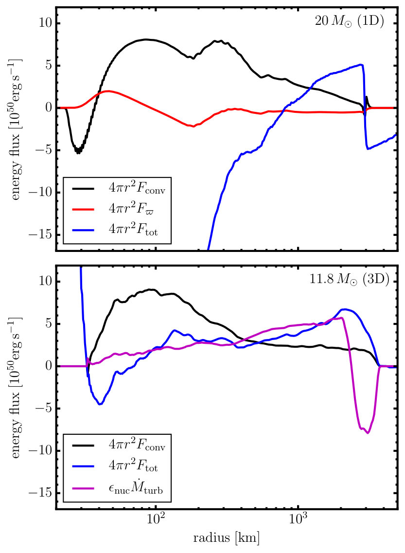 Figure 1
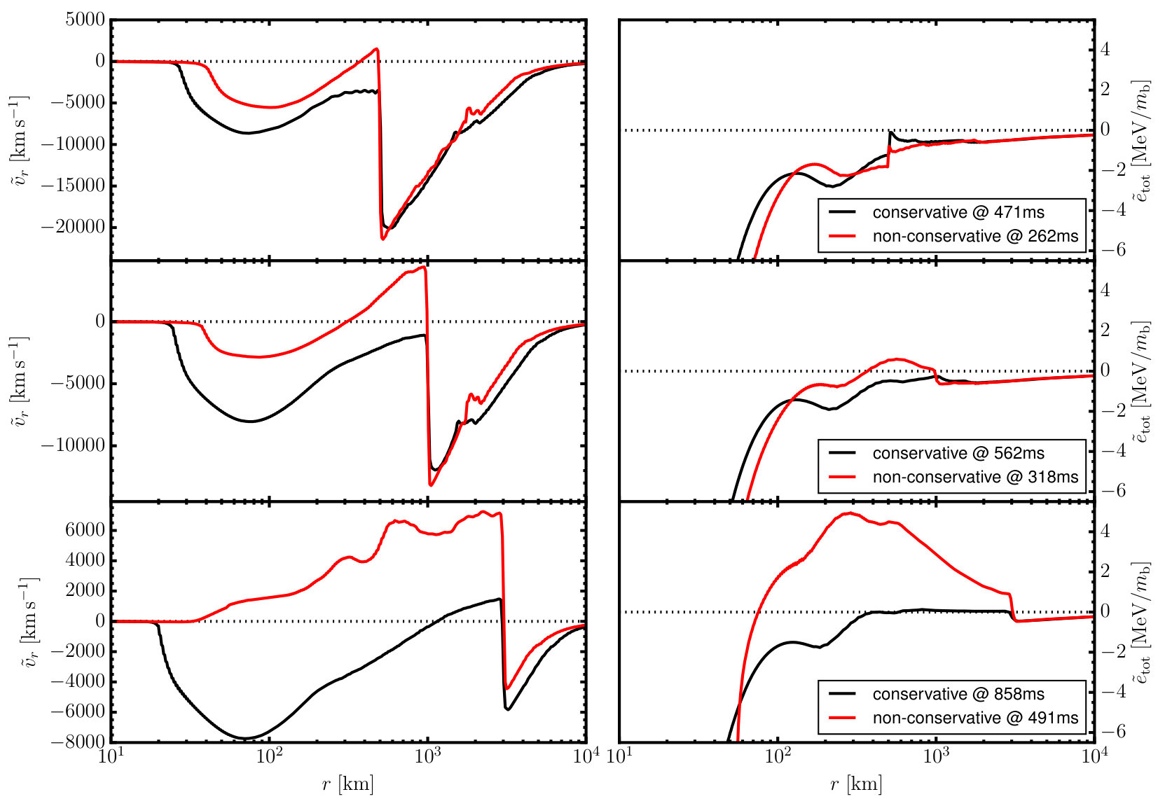 Figure 2
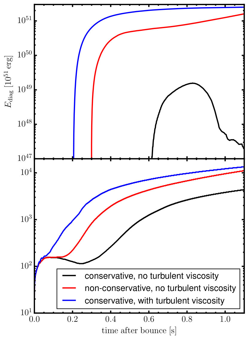 Figure 3
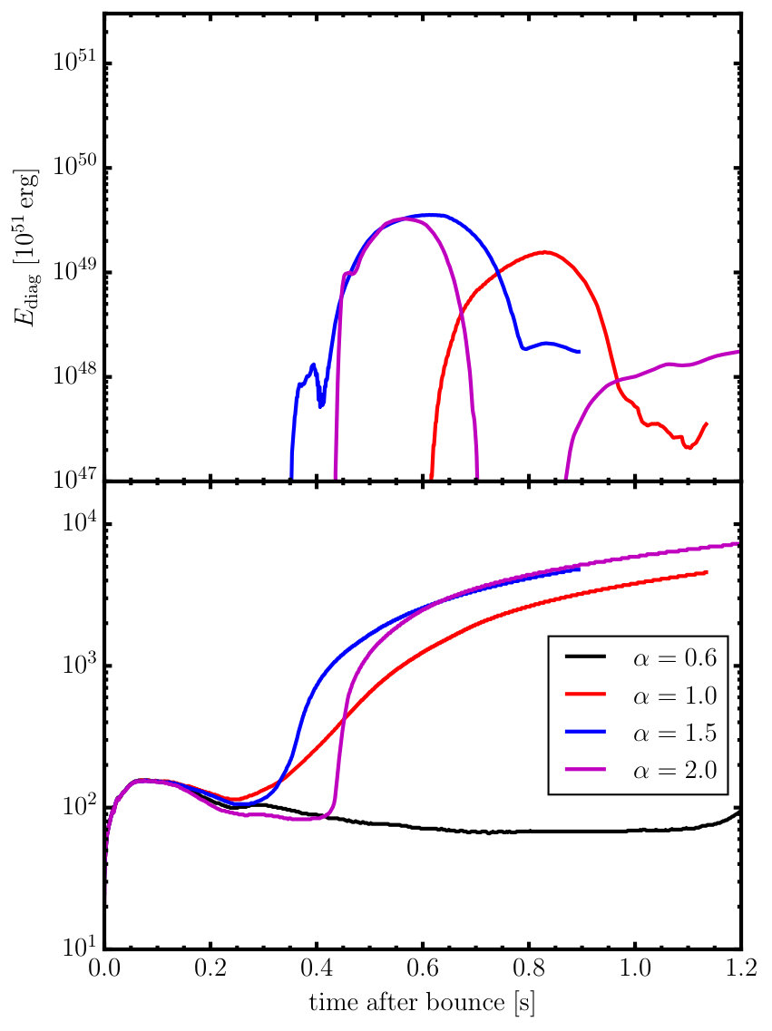 Figure 4
Peer Reviews
No public reviews on file for this paper yet. If you reviewed it on a platform where reviews are public (OpenReview, ICLR, NeurIPS, ICML), you can paste yours below so the community can read it here.
Videos
No videos yet. Explain this paper in a talk, walkthrough, or lecture? Add one.
A Critical Assessment of Turbulence Models for 1D Core-Collapse Supernova Simulations
Bernhard Müller1
1Monash Centre for Astrophysics, School of Physics and Astronomy, Monash University, Victoria 3800, Australia
[email protected] E-mail: [email protected]
Abstract
It has recently been proposed that global or local turbulence models can be used to simulate core-collapse supernova explosions in spherical symmetry (1D) more consistently than with traditional approaches for parameterised 1D models. However, a closer analysis of the proposed schemes reveals important consistency problems. Most notably, they systematically violate energy conservation as they do not balance buoyant energy generation with terms that reduce potential energy, thus failing to account for the physical source of energy that buoyant convection feeds on. We also point out other non-trivial consistency requirements for viable turbulence models. The model of Kuhfuss (1986) proves more consistent than the newly proposed approaches for supernovae, but still cannot account naturally for all the relevant physics for predicting explosion properties. We perform numerical simulations for a progenitor to further illustrate problems of 1D turbulence models. If the buoyant driving term is formulated in a conservative manner, the explosion energy of for the corresponding non-conservative turbulence model is reduced to even though the shock expands continuously. This demonstrates that the conservation problem cannot be ignored. Although plausible energies can be reached using an energy-conserving model when turbulent viscosity is included, it is doubtful whether the energy budget of the explosion is regulated by the same mechanism as in multi-dimensional models. We conclude that 1D turbulence models based on a spherical Reynolds decomposition cannot provide a more consistent approach to supernova explosion and remnant properties than other phenomenological approaches before some fundamental problems are addressed.
keywords:
supernovae: general – convection – hydrodynamics – turbulence – stars: massive
††pagerange: A Critical Assessment of Turbulence Models for 1D Core-Collapse Supernova Simulations–LABEL:lastpage††pagerange: A Critical Assessment of Turbulence Models for 1D Core-Collapse Supernova Simulations–23
1 Introduction
According to our present understanding, the explosions of massive stars as core-collapse supernovae depend critically on the breaking of spherical symmetry in the supernova core (Janka, 2012; Foglizzo et al., 2015; Müller et al., 2016b) except in the case of the least massive progenitor stars (Kitaura et al., 2006). In the neutrino-driven paradigm, the breaking of spherical symmetry is mediated by two instabilities, namely buoyancy-driven convection (Herant et al., 1994; Burrows et al., 1995; Janka & Müller, 1995) and the standing-accretion shock instability (Blondin et al., 2003; Foglizzo et al., 2007), which manifests itself in the form of global sloshing or spiral motions of the shock. The resultant multi-dimensional (multi-D) fluid flow aids neutrino heating through a variety of interrelated effects, e.g. by mixing hot neutrino-heated and colder material from the vicinity of the shock, by providing turbulent pressure (Burrows et al., 1995; Murphy et al., 2013), by providing heating close to the shock by secondary shocks (Müller et al., 2012b), and by turbulent dissipation (Mabanta & Murphy, 2018).
There have been attempts to distil these effects back into an effective one-dimensional (1D) description using an appropriate turbulence model. On the one hand, such a 1D turbulence model for the supernova core may lead to a better conceptual understanding of the role of multi-D effects (Murphy & Meakin, 2011; Mabanta & Murphy, 2018). On the other hand, one might hope that effective 1D models of neutrino-driven supernovae could provide an efficient way to predict the “explodability” and even the explosion properties across a population of progenitor models at a cheaper cost than full-blown multi-D models, but with greater rigour and consistency than more parameterised approaches like those of O’Connor & Ott (2010); Ugliano et al. (2012); Perego et al. (2015); Sukhbold et al. (2016); Müller et al. (2016a).
The simplest approach of adopting the mixing-length theory (MLT) for stellar convection (Biermann, 1932; Böhm-Vitense, 1958) to the supernova problem already dates back to the 1980s (Mayle, 1985; Wilson & Mayle, 1988). However, the extra convective energy transport provided by convection within the framework of MLT alone does not improve the heating conditions to such a degree as to allow explosions in spherical symmetry (Hüdepohl, 2014; Mirizzi et al., 2016).
More general turbulence models have been proposed to capture multi-D effects in the heating region more adequately (Murphy et al., 2013; Mabanta & Murphy, 2018). Only recently have there been efforts to use such turbulence models predictively. Mabanta & Murphy (2018) incorporated a 1D turbulence model into steady-state solutions for the accretion flow onto a proto-neutron star to derive the reduction of the critical neutrino luminosity for shock revival (Burrows & Goshy, 1993) due to multi-D effects. Following up on their earlier work, Mabanta et al. (2019) went on to include a simple turbulence model in dynamical simulations with a view to studying the explodability of supernova progenitors. Using a light-bulb model for neutrino heating and cooling, they found that their turbulence model roughly reproduces the reduction of the critical luminosity in multi-D for a reasonable choice of model parameters. Shortly thereafter, Couch et al. (2019) presented a time-dependent 1D turbulence model, which they coupled to the neutrino transport code of O’Connor & Couch (2018) and then used to explore the systematics of explodability, and explosion and remnant properties across the stellar mass range. One might thus hope that such effective 1D turbulence models can furnish a more “consistent” approach to the progenitor-explosion connection than current phenomenological models.
In this paper, we critically examine this idea. We shall argue that consistency and crucial physical principles such as energy conservation are difficult to achieve, especially during the explosion phase. We show that even the time-dependent approach of Couch et al. (2019) still suffers from inconsistencies. To remedy these, one can draw on the extensive literature on generalisations of mixing-length theory, which have been studied since the 1960s (e.g. Spiegel, 1963; Unno, 1967; Eggleton, 1983; Kuhfuss, 1986; Gehmeyr & Winkler, 1992; Canuto, 1993; Canuto & Dubovikov, 1998; Wuchterl & Feuchtinger, 1998). Classic time-dependent convection models as developed by Kuhfuss (1986) and Wuchterl & Feuchtinger (1998) offer solutions to most of the inconsistencies in the models of Mabanta et al. (2019) and Couch et al. (2019), but even then the behaviour of 1D turbulence models during the explosion phase is not fully satisfactory. We illustrate the remaining problems for a progenitor by implementing the model of Kuhfuss (1986) in the neutrino hydrodynamics code CoCoNuT (Müller et al., 2010; Müller & Janka, 2015) with some necessary adaptations for the core-collapse supernova problem. The goal of our analysis and our numerical experiments is primarily to illustrate the pitfalls that crop up when one seeks to model supernova explosions in 1D by including the effects of turbulence. We do not aim to present a consistent solution to all of these problems, which does not appear within reach at the moment.
This paper is organised as follows: In Section 2 we discuss recently proposed 1D turbulence models and analyse to what extent they meet important physical consistency criteria. In Section 3, we discuss the 1D turbulence model of Kuhfuss (1986) and show that it meets essential physical consistency criteria such as total energy conservation and compatibility with the second law of thermodynamics. We also describe its implementation in the hydrodynamics code CoCoNuT. We then present results for a star as test case using several variations of the turbulence model of Kuhfuss (1986) in Section 4 and conclude by discussing future perspectives for 1D explosion modelling in Section 5.
2 Recent 1D Turbulence Models for Core-Collapse Supernovae
Both Mabanta et al. (2019) and Couch et al. (2019) start from a spherical Reynolds decomposition of the fluid equations, from which they discard some higher-order terms before they apply closure relations. Specifically, they ignore the turbulent mass flux in the spirit of the anelastic approximation, so that no turbulent correlation terms appear in the continuity equation. The common starting point for both models can be written as
[TABLE]
Here , , , and denote the fluid density, velocity, pressure, and total (internal+kinetic) energy density, denotes the gravitational acceleration, and is the volumetric neutrino heating rate. and are the Reynolds stress tensor and the turbulent energy flux obtained from the Reynolds decomposition. Spherical Reynolds averages are denoted by angled brackets, or by carets for individual variables. Primes, as used in the term for buoyant energy generation, denote fluctuating quantities.
2.1 Model of Mabanta
et al. (2019)
Mabanta et al. (2019) impose a closure relation by essentially assuming that the magnitude of turbulent radial velocity fluctuations is constant within the gain region, and that turbulent dissipation balances buoyant energy generation if integrated over the entire gain region. With buoyant driving parameterised as in terms of the volume-integrated heating rate and a calibrated parameter , and turbulent dissipation scaling as in terms of the typical value of velocity perturbations (which can formally defined as a root-mean-square average ) and an effective dissipation length (taken to be the width of the gain region), one obtains
[TABLE]
as also derived by Müller & Janka (2015). The Reynolds stress tensor is assumed to be diagonal with equipartition between the radial and non-radial components so that and . The turbulent dissipation is also used to supply the source term for buoyant energy generation in Equation (3).
To obtain the convective flux, Mabanta et al. (2019) use a fit for the convective luminosity that is inspired by an analysis of multi-D simulations,
[TABLE]
Here is the radial coordinate, is the gain radius, is an appropriately chosen transition width, and is a calibrated dimensionless parameter. Mabanta & Murphy (2018) use Equation (5) only up to the shock, where plummets to zero. The term for the work exerted by Reynolds stresses is neglected in the energy equation.
Although the prescriptions for the Reynolds stresses and the convective luminosity are in line with multi-D simulations, there is an obvious question about energy conservation in this model. Integrating Equation (3) under the assumption that turbulent dissipation locally balances buoyant energy generation results in
[TABLE]
The work done by gravitational forces on the spherically averaged flow does not violate energy conservation and cancels if gravitational potential energy is included in the budget (Shu, 1992). Similarly, the contribution of neutrino heating does not violate total energy conservation if it is obtained from a conservative neutrino transport scheme. However, the turbulence model introduces an extra source term that violates energy conservation. As we shall see, such a source term also appears in the model of Couch et al. (2019).
It has been argued (Q. Mabanta, private communication; Couch et al., 2019) that energy is still effectively conserved if one accounts for the available free energy associated with convectively unstable gradients. Although this argument is not entirely incorrect, it does not convincingly justify the use of a 1D turbulence model that does not manifestly conserve energy, but rather points to a loophole in the model: In the full multi-D problem, energy is always strictly conserved, so the reservoir of available free energy associated with unstable gradients must be depleted as turbulent kinetic energy grows. Convective motions feed on work of the expanding and contracting bubbles analogous to a heat engine (Herant et al., 1994; Müller & Janka, 2015), and on the gravitational potential energy of the bubbles, i.e., the reservoir of free energy associated with unstable gradients forms a part of the reservoir of internal and potential energy. Any increase in turbulent kinetic energy must therefore be balanced by a decrease in internal or potential energy. To ensure total energy conservation, a 1D turbulence model needs to reflect this reshuffling of internal and potential energy by consistently including all the necessary turbulent correlation terms. If there is a source term for the turbulent kinetic energy, there must be a corresponding sink term for internal or potential energy to account for the fact that the available reservoir of free energy associated with unstable gradients is drained as convective motions develop.
But on the other hand, the source term in the Reynolds-averaged energy equation (3) is formally correct, so how is it possible that the multi-D hydro equations conserve total energy whereas the spherically Reynolds-averaged equation do not? The answer is that the system (1-3) does not include all terms from the Reynolds decomposition consistently: Specifically, it ignores the turbulent mass flux in Equation (1) and thus neglects the (instantaneous) reduction of potential energy due to changes in the density profile, but includes it in the source term in Equation (3). In Section 3, we shall further discuss to what extent this problem can be fixed.
There is another potential issue with the model of Mabanta et al. (2019). If Equation (5) for the convective luminosity is only used up to the shock, then this implies that the term in the energy equation will have a delta-function spike at the shock, and it is unclear whether such a feature can be handled properly by the hydrodynamics solver, i.e. whether it affects the propagation speed of the shock in an unphysical manner.
2.2 Model of Couch
et al. (2019)
Couch et al. (2019) solve a separate evolution equation for the turbulent velocity fluctuations and compute the turbulent flux in the energy equation using an MLT closure. They assume the same closure for the Reynolds stress tensor as Mabanta et al. (2019). In their model, the momentum and energy equations come down to
[TABLE]
where we have neglected the neutrino momentum source term, which is irrelevant for our discussion. Here is an MLT diffusion coefficient, and the mixing length is chosen as a multiple of the pressure scale height , where is a tunable parameter of order unity. Note that we have tacitly corrected a typo in their Equation (26), where the term should not be multiplied by the radial velocity . There is likely another typo in their Equation (25), which should contain a fictitious force term on the right-hand side (RHS). Moreover, the energy equation appears to assume an isotropic Reynolds stress tensor, and is inconsistent with the assumed form of . However, these problems are somewhat peripheral to our further discussion.
For the evolution of the turbulent kinetic energy, Couch et al. (2019) propose the following equation:
[TABLE]
Here, the turbulent dissipation term appears as a local sink term, and the source term is expressed in terms of the Brunt-Väisälä frequency in a manner consistent with classical, time-dependent MLT (cp. Section 2.1 in Müller et al. 2016b).
Including a separate time-dependent equation for the turbulent kinetic energy makes the reshuffling of energy between the spherically-averaged bulk flow and the turbulent fluctuations more transparent, but still does not solve the problem of energy conservation, and even introduces further ambiguities. From the form of the equations and the discussion in Couch et al. (2019) it appears that in the energy equation (8) is not meant to include the turbulent kinetic energy, so that one needs to add Equations (8) and (9) to analyse total energy conservation. As in Section 2.1, this again leads to an additional source term that breaks total energy conservation. Since the typical turbulent velocity must be related to the amount of neutrino heating just as in multi-D in order to maintain a stationary, slightly superadiabatic gradient, the rate of artificial energy injection by buoyant driving is also of the same scale as before, i.e. roughly of order of the volume-integrated neutrino heating rate itself.
Moreover, the model leaves us with a consistency problem. While it is implicitly assumed that does not include the turbulent kinetic energy – which is why the dissipation term appears as a source in Equation (8) – the term for the work done by Reynolds stresses is written as a divergence in Equation (3). In Equation (3), however, implicitly includes the turbulent kinetic energy as correctly recognised in Mabanta et al. (2019). If one subtracts the turbulent kinetic energy equation from the total energy equation, one must instead treat Reynolds stresses as a body force so that their contribution on the RHS of the energy equation is instead of (see also below in Section 3).
This may seem a trivial issue, but it is enlightening to analyse its potential repercussions. Assuming for the sake of simplicity that the turbulent pressure is actually isotropic, then including the work of Reynolds stresses as a divergence as in Equation (8), implies that the evolution equation for the internal energy density of the spherically symmetric bulk flow is changed to
[TABLE]
in the absence of heating and cooling terms from neutrinos and dissipation, instead of
[TABLE]
This is tantamount to an artificial entropy source term
[TABLE]
It is noteworthy that this term can become negative, i.e. the turbulence model implicitly allows for a decrease of entropy even in the absence of physical source terms for cooling.
There is yet another problem with the model of Couch et al. (2019) that concerns the convective energy flux . The model essentially assumes that can be computed by extrapolating the total energy density to the original position of the convective bubbles using the local gradient to obtain the fluctuating part ,
[TABLE]
This, however, leads to unphysical results. Let us first consider the fluctuations of the internal energy density . To obtain the correct MLT flux, one needs to account for the done by the convective bubbles as they contract and expand while adjusting to the ambient pressure (Hüdepohl, 2014; Mirizzi et al., 2016). If the expansion/contraction is adiabatic, one obtains
[TABLE]
By expressing in terms of the entropy and density gradients using the first law of thermodynamics, one obtains an important corollary: If the entropy gradient vanishes, then the convective energy flux also vanishes (assuming that there are no composition gradients). If one uses Equation (13) this is no longer guaranteed.
There is also a concern about the turbulent transport of bulk kinetic energy: This effect is included in Equation (8) via Equation (13), but there is no corresponding term for the turbulent transport of momentum (i.e. turbulent viscosity) in Equation (8).
3 The Energy-Conserving Turbulence Model of Kuhfuss (1986)
3.1 Description and Discussion of Individual
Terms
Most of the problems discussed in Sections 2.1 and 2.2 are in fact nicely solved by time-dependent one-equation turbulence models that have been developed for stellar evolution (Stellingwerf, 1982; Kuhfuss, 1986; Wuchterl & Feuchtinger, 1998), originally motivated by the problem of pulsations of RR Lyrae stars and Cepheids. Here we shall use the work of Kuhfuss (1986) (with some modifications by Wuchterl & Feuchtinger 1998) as a starting point. In their approach, the momentum equation in conservation form can be written as
[TABLE]
The underlying assumption about the form of the Reynolds stress tensor differs slightly from Mabanta et al. (2019) and Couch et al. (2019); it is decomposed into a trace component – the turbulent pressure – and a trace-free component modelled after the viscous Navier-Stokes equations. This trace-free term gives rise to the additional turbulent viscosity term on the RHS with a turbulent dynamic viscosity111Note that our notation is different from Kuhfuss (1986), where is used for the kinematic turbulent viscosity. , which is expressed in the spirit of MLT as , where is a dimensionless coefficient of order unity. Although the assumed form of the trace-free term can be criticised as ad hoc, it has the virtue of ensuring that it can be matched with a viscous term in the energy equation that can be expressed as a flux divergence (to ensure energy conservation) and always results in an increase of fluid entropy.
Kuhfuss (1986) and Wuchterl & Feuchtinger (1998) also formulate an evolution equation for the turbulent kinetic energy . With one important modification, the equation for can be written as
[TABLE]
in Eulerian form. Here, and are dimensionless coefficients for the turbulent diffusion of turbulent kinetic energy and turbulent dissipation. Different from Kuhfuss (1986) and Wuchterl & Feuchtinger (1998), we have omitted the viscous dissipation term from the turbulent kinetic energy equation. Although it seems plausible that the turbulent viscosity should should initially feed kinetic energy from the bulk flow into disordered small-scale motion (i.e. into turbulent kinetic energy), this has undesirable consequences. The problem is that the viscous heating term is linear in just like the buoyant driving term. If included in the equation for , it would act like a destabilising gradient wherever (i.e. almost everywhere) with taking the place of the Brunt-Väisälä frequency as the growth rate. From the viewpoint of numerical stability, such behaviour would be disastrous at the shock, but it is also clearly unphysical. Shifting the viscous heating term to the internal energy equation seems the only viable solution.
Like Equation (9), the turbulent energy equation includes terms for the advection and the turbulent diffusion of turbulent kinetic energy (the two flux divergence term on the left-hand side). However, there is also a term that effectively accounts for term on the “eddy gas”. Including this term in Equation (16) ensures that the work exerted by the turbulent pressure correctly enters as in the corresponding equation for without turbulent kinetic energy, and hence does not change the internal energy density of the bulk flow. Apart from dimensionless coefficients of order unity, the source term for buoyant driving and the dissipation term are essentially the same as in Equation (9); the driving term can again be expressed in terms of the Brunt-Väisälä frequency as .
In the theory of Kuhfuss (1986), total energy conservation is ensured by consistently including the mass-specific turbulent kinetic energy in the energy equation. Kuhfuss (1986) originally formulated an extended internal energy equation including as the internal energy of an “eddy gas”, but this equation can be easily recast into a total energy equation analogous to Equation (3),
[TABLE]
Here, and denote the convective flux of internal energy and turbulent kinetic energy, and is the energy flux from viscous turbulent stresses. Equation (17) is manifestly conservative because all the turbulent effects are lumped into flux divergence terms. In accordance with Equation (14), the convective energy flux is calculated as
[TABLE]
where is another adjustable dimensionless parameter for turbulent energy transport. The viscous energy flux is given by
[TABLE]
and as per Equation (16), the convective flux of turbulent kinetic energy is
[TABLE]
For further analysis, it is useful to consider the internal energy equation for the spherical background flow as well, which reads
[TABLE]
where is another dimensionless coefficient of order unity and Equation (14) has been used to express the convective flux of internal energy. Note that the viscous dissipation term appears in the internal energy equation for reasons explained above.
Equations (17), (16), and (21) ensure that i) entropy is conserved during expansion and contraction in the absence of diffusive flux and source/sink term, that ii) the convective flux transports energy into the direction of negative entropy gradients, and that iii) total energy is conserved. Energy conservation is achieved by including a sink term due to buoyant driving in the internal energy equation, and not including a source term for buoyant driving in the total energy equation.
3.2 The Kuhfuss Model Interpreted in the Framework
of Favre Decomposition
It may appear as though the solution for energy conservation in the model of Kuhfuss (1986) were somewhat ad hoc and still inconsistent, because it merely relies on neglecting the turbulent mass flux in different equations than Mabanta et al. (2019) and Couch et al. (2019). But this appearance is deceptive. The Kuhfuss model is in fact consistent if we re-interpret the equations as arising from a Favre decomposition of the flow based on mass-weighted averages (Favre, 1965) for mass-specific quantities (e.g., , , , and mass fractions ) instead of a Reynolds decomposition. Using tildes to denote Favre averages for any variable and double primes for fluctuations around Favre averages, the equations for conservation of mass, momentum, energy, partial masses, and for the turbulent kinetic energy read,
[TABLE]
as derived in Appendix A. Note that the turbulent kinetic energy is now defined as the Favre average /2.
The only terms that are not mirrored222 Bear in mind that the Reynolds stress tensor is broken up into a trace part and a trace-free part in the Kuhfuss model. in the model of Kuhfuss (1986) are the ones containing turbulent fluctuations of the pressure due to the assumption of instant horizontal pressure equilibration. Different from the Reynolds-decomposed equations, the total mass flux factorises as . This eliminates both the turbulent mass flux term from the continuity equation and the term from the total energy equation, while still naturally appears as a source term in the kinetic energy equation. Thus, the choice of discarding the term in the energy equation is not actually an approximation in the model of Kuhfuss (1986), and there is in fact no need to include extra terms in the Kuhfuss model to achieve full consistency with the spherically-averaged fluid equations. Instead, we simply need to treat some of the evolved quantities in the Kuhfuss model as Favre averages and solve the following equations for mass, momentum, internal energy, partial mass fractions , and turbulent kinetic energy :
[TABLE]
[TABLE]
[TABLE]
[TABLE]
[TABLE]
Here, the turbulent viscosity is defined analogously to Section 3.1 as , and for reasons explained above, we still prefer to feed the energy from turbulent viscous dissipation directly into internal energy. Note that one can also formulate an equation for the mole fractions instead of Equation (30); its form is completely analogous.
To close the system, we assume that the root-mean-square radial velocity fluctuations are related to the total turbulent kinetic energy as , reflecting the rough equipartition between radial and non-radial velocity fluctuations in multi-D simulations. Different from Kuhfuss (1986), we shall use (as originally proposed by Stellingwerf 1982) in our numerical implementation, which makes for a larger force from the turbulent pressure gradient in the momentum equation. Although this is somewhat inconsistent, it does not fundamentally alter the structure and properties of the turbulence model. The source term can be expressed as using the MLT density contrast 333Note that this is equivalent to the expression ussed in 2.2.
[TABLE]
The model contains six adjustable non-dimensional parameters, namely as the ratio of the mixing length to the pressure scale height, and the coefficient for turbulent dissipation, for the turbulent viscosity, and , , and for the turbulent transport of bulk energy, mass fractions, and turbulent kinetic energy. In our implementation, we shall set all of these coefficient to unity () except for the mixing-length coefficient . In fact, we shall see that must hold for consistency reasons given the assumed form of the term for buoyant driving.
3.3 Compatibility with the Second Law of
Thermodynamics
In the light of our discussion of entropy conservation earlier in this paper, the form of the Equations (27-31) appears puzzling at first glance: It is easy to see that the additional terms from turbulent stresses, turbulent viscosity, and turbulent dissipation either conserve or generate entropy and are thus compatible with the second law of thermodynamics. The sink term from buoyant driving in the internal energy generation seems to violate the second law, however. It appears that the price for energy conservation is the possibility of a decrease in entropy in the bulk flow due to the generation of turbulent kinetic energy, i.e. a violation of the second law of thermodynamics. This is especially curious since we cannot blame this sink term on the inconsistent treatment of the turbulent mass flux anymore, which has simply disappeared in the Favre decomposition.
The solution to this conundrum is that this sink term cancels an extra entropy source term that emerges from the convective energy flux term. In order to see this, let us first determine the change of entropy due to the convective transport (denoted by the subscript “conv”) of energy and mole fractions. It is convenient to consider the convective derivative of thermodynamic quantities, whieh can be obtained from the fluxes in the conservation equations in a straightforward manner, e.g.,
[TABLE]
for the internal energy. It is also advantageous not to spell out the del operator in spherical polar coordinates. With these considerations in mind, we obtain the rate of change of the fluid entropy due to turbulent transport as
[TABLE]
where denotes the chemical potential for species (and not the turbulent viscosity).444Note that in the strictest sense the thermodynamic quantities , , and are not Favre/Reynolds averages, but functions of the Favre/Reynolds averages of , , and , i.e. they are to be understood as , and so forth.
For this to be a conservation equation, we would need the RHS to be of the form , where is an MLT turbulent entropy flux proportional to . We can obtain such a term by means of rearrangements on the RHS if (which we shall always assume henceforth), but are then left with an extra term,
[TABLE]
Expressed as a Eulerian equation for , this becomes
[TABLE]
Now consider the entropy change due to the sink term from buoyant driving (subscript “buoy”) in the internal energy equation (29),
[TABLE]
In order to obtain a form containing quadratic terms in some gradients of thermodynamic quantities as in Equation (35), we assume hydrostatic equilibrium so that we can replace with :
[TABLE]
In fact, there is some motivation for consistently using as the effective gravity for non-hydrostatic flow because this ensures that the growth rate of turbulent kinetic energy is compatible with the growth rate of the compressible Rayleigh-Taylor instability (for which see, e.g., Bandiera 1984; Benz & Thielemann 1990; Müller et al. 1991; Zhou 2017).
After expanding in terms of the partial derivatives of with respect to , , and , the term cancels out, and we obtain
[TABLE]
We can then exploit Maxwell’s relations555 Note that one can use for all derivatives with respect to . and to replace the thermodynamic derivatives of ,
[TABLE]
We can further rewrite this as
[TABLE]
The terms in the first line cancel the extra source term in if and only if and . Thus, only the terms in the second and third line remain as a net source or sink term for the entropy. In order to better understand these terms, we reformulate them in terms of the MLT entropy and mole fractions contrasts and by eliminating in favor of the convective turnover time ,
[TABLE]
The terms in the second and third line can be identified as the contribution of the mixing entropy for material with and , which is liberated per convective turnover time. This is demonstrated in Appendix B for a general multi-species fluid (cp. § 21 in Landau & Lifschitz 1969 for the case of constant composition).
For well-behaved equations of state the mixing entropy is always positive; thus the Kuhfuss model actually predicts the correct positive entropy change due to turbulent mixing. This is particularly easy to see for the case without composition gradients, in which case the sum of Equations (36) and (41) reduces to
[TABLE]
where is the heat capacity at constant pressure.
This analysis of the entropy source term shows that the Kuhfuss model is compatible with the second law, providing the correct, unavoidable rate of entropy generation in the absence of turbulent dissipation and turbulent viscosity. Including a source term for buoyant driving in the total energy equation therefore also overestimates entropy generation by turbulent mixing and dissipation. Moreover, and are actually not free parameters, they are fixed by the coefficient of the buoyant driving term and the requirement of a correct entropy generation rate from turbulent mixing. Only the “equation of state” of the turbulent “eddy gas”, , , and the mixing length parameter remain as free parameters (unless there are further, yet undiscovered consistency requirements).
We need to stress, however, that consistency with energy conservation and with the second law does not mean that the Kuhfuss model is accurate for the supernova problem. The closure relations in the model are still based on an MLT ansatz that may not be valid in the regime of strong compressibility and for the typical flow geometry encountered in supernova explosions. Constructing appropriate closures for the turbulent fluctuations that include compressibility effects is anything but trivial (see, e.g., Canuto 1993, and also Duffell 2016 for a thoughtful attempt in the case of the compressible Rayleigh-Taylor instability).
3.4 Numerical Implementation
In order to illustrate the explosion dynamics of 1D models that incorporate effects of turbulence, we implement the model from Section 3.2 in the neutrino radiation hydrodynamics code CoCoNuT-FMT (Müller et al., 2010; Müller & Janka, 2015) and run three different variations of the model for the progenitor of Woosley & Heger (2007). CoCoNuT-FMT is a finite-volume code for general relativistic hydrodynamics in spherical polar coordinates with the xCFC approximation for the metric (Cordero-Carrión et al., 2009). It uses higher-order reconstruction and an approximate Riemann solver combined with a stationary, fast multi-group neutrino transport (FMT) scheme as described in Müller & Janka (2015).
Since CoCoNuT-FMT is a relativistic code, some care is required to implement the turbulence model from Section 3, which is formulated in the Newtonian approximation. Since general relativistic effects are unimportant and velocities are well below the speed of light in the gain layer as the main region of interest, one can dispense with a detailed re-derivation of the equations in full relativity and simply include a few heuristic modifications: All flux terms pick up an extra factor in terms of the lapse function and the conformal factor of the conformally flat metric, and all conserved quantities pick up an extra factor . Moreover, we use the relativistic expression for the MLT density contrast (cp. Müller et al., 2013),
[TABLE]
when computing the Brunt-Väisälä frequency and buoyant driving. Whether one computes the gravitational acceleration simply as the derivative of the lapse function or includes relativistic correction factors is immaterial in practice.
The terms in the turbulence model are implemented in an operator-split approach except for the convective energy flux and the corresponding turbulent fluxes in the equations for the mass fractions and the Favre-averaged electron fraction ; these are added directly to the hydro fluxes obtained from the Riemann solver.
The operator-split update of the turbulent kinetic energy and the bulk fluid energy and momentum are staged as follows: We first integrate the terms for buoyant energy generation and dissipation,
[TABLE]
Here we deviate from Kuhfuss (1986) and Wuchterl & Feuchtinger (1998) by introducing a dissipation length that may be different from the mixing length . The rationale for this is that the identification of and can lead to excessive overshoot into the convectively stable atmosphere of the proto-neutron star. We limit the dissipation length by balancing the turbulent kinetic energy and the work against buoyancy for overshooting by a distance ,
[TABLE]
This is motivated by the realisation that the penetration depth of convective plumes from the gain region is not simply a fixed multiple of the pressure scale height, but regulated by the kinetic energy of the overshooting plumes and the Brunt-Väisälä frequency in the convectively stable cooling layer (Murphy et al., 2009, see their Equation 26). This limiting procedure for the dissipation length is only applied in regions where indicates convective stability.
Since the source term for buoyant driving vanishes for , care must be taken to ensure that convective motions can actually grow. One possibility is to imposes a small seed value for as done by Couch et al. (2019). We instead circumvent this problem altogether by evolving , whose evolution equation can be obtained using the chain rule:
[TABLE]
No seed for is required since is non-zero even for . Since this equation is stiff if is very small, we solve for the value at the next time step implicitly, and afterwards solve
[TABLE]
by updating the internal energy as
[TABLE]
As discussed in Section 3.3, one can argue that should actually replace as the effective gravitational acceleration in the source term for buoyant driving in the turbulent kinetic energy equation (31) and in the calculation of the Brunt Väisälä frequency. This would have the virtue that the direction of unstable gradients would reverse once the pressure gradient behind the shock becomes positive as in the case of Rayleigh-Taylor later during the explosion (Chevalier, 1976; Müller et al., 1991; Fryxell et al., 1991). Using as the effective gravity can, however, create numerical problems at the shock, and following late-time mixing instabilities would also require other changes in the model assumptions, e.g., on the mixing length (Duffell, 2016). For this reason, we still choose to compute the Brunt-Väisälä frequency using the gravitational acceleration instead of .
We next update the fluid velocity according to
[TABLE]
and then perform a step for diffusion, advection, and work,
[TABLE]
Finally, we integrate the turbulent viscosity terms,
[TABLE]
and convert back from the primitive variables to the conserved variables in general relativity,
4 Numerical Results
We evolve the progenitor of Woosley & Heger (2007) until after collapse and then switch on the turbulence terms. We compare three variations of the turbulence model described in Sections 3.2 and 3.4:
- •
As a baseline model, we consider a case where turbulent viscosity is switched off.
- •
As a second case, we run another model without turbulent viscosity, where we switch off the sink term for buoyant driving in the internal energy equation at after bounce. In other words, instead of Equation (48), we solve
[TABLE]
as in Couch et al. (2019). This case illustrates the effect of energy non-conservation.
- •
In a third simulation, we revert to the conservative formulation of buoyant driving and switch on turbulent viscosity.
All the dimensionless parameters are set to unity in those three cases, i.e. .
In addition, we also investigate the influence of the mixing-length parameter in the conservative case without turbulent viscosity in another three runs with , , and while keeping (as well as as dictated by consistency requirements, see Section 3.3).
Figure 1 compares the shock trajectories and diagnostics explosion energies for the first three cases. Following the usual definition (Buras et al., 2006; Müller et al., 2012a), we compute as the total (internal+kinetic+potential) energy of the material that is nominally unbound at a given time. The turbulent kinetic energy is included in the total energy.
4.1 Impact of Energy Non-Conservation
The shock is revived in all three cases, but the explosion dynamics is significantly different. Comparing the two runs with and without the sink term for buoyant driving in the internal energy equation, we find that ignoring energy conservation in turbulence models has serious repercussions. Shock revival occurs more than later for the energy-conserving turbulence model.
What is even more concerning, however, is that the rise of the explosion energy after shock revival is completely different. With the conservative formulation of the buoyant driving term, grows slowly to reach little more than of . The diagnostic energy then decreases again so that the ejecta are only marginally unbound in the end. Even though the shock continuously propagates outward, the result is only a fizzle and not a full-blown explosion. Figure 3 provides more explanation for this behaviour by comparing profiles of the total specific energy and radial velocity from the conservative and non-conservative model for similar shock radii. For a given shock radius, the conservative model consistently exhibits lower and radial velocity behind the shock. The turbulent flux terms and the turbulent pressure evidently alter the thermodynamic conditions on the downwind side of the shock sufficiently to maintain continuous shock expansion, but without pumping an appreciable amount of energy into the ejecta.
The late-time behaviour of the case with a non-conservative formulation of the buoyant driving term is particularly disturbing as it is clearly unrealistic. Initially, the rise of slows down as physically expected from a declining neutrino heating rate with a visible break around a post-bounce time of . A few hundreds of miliseconds later, however, again starts to increase at an accelerated rate.
These findings lead to two conclusions: First, the question of total energy conservation clearly must not be ignored when formulating a 1D turbulence model for supernova explosions; it is crucial for the energetics of the explosion. Second, correctly reproducing the energetics within a 1D turbulence model is evidently a very different matter than merely reproducing shock revival and shock expansion in a seemingly realistic way. It is non-trivial to ensure that the shock propagation is coupled to the explosion energetics in the same manner as it is in multi-D simulations, where the shock velocity roughly follows the analytic scaling law derived by Matzner & McKee (1999),
[TABLE]
in terms of , the mass between the shock and the gain radius, and the pre-shock density as shown by Müller (2015). The conservative model without turbulent viscosity does not ensure this, and is therefore also unsatisfactory.
One might suspect that the low explosion energy in the conservative case is just an accidental pathology due to an unfortunate choice of the non-dimensional parameters. Varying the mixing-length parameter does not qualitatively change the behaviour of the model, however. Figure 2 shows that the explosion energy remains unacceptably low even if we vary over a wide range from to . Whether different choices for and could remedy the problem of fizzling explosions is a moot point; if this were the case, one could still justifiably doubt the robustness of a model that can easily behave in an unsatisfactory manner.
As an aside, Figure 2 reveals that the simulations do not react monotonically to changes in if is varied over a wider range than in Couch et al. (2019). The models with and actually explode later than the one with , but then result in faster shock expansion once the explosion sets in. Although this may seem puzzling at first glance, such a non-monotonic behavior is not unexpected. As is increased, buoyant driving becomes stronger for the same superadiabatic gradient, but on the other hand mixing becomes more effective at flattening the unstable gradient in the gain region for a given turbulent velocity, which in turn reduces buoyant driving. If is increased sufficiently, the net result of these two competing effects can be, at least in certain situations, a decrease of the turbulent pressure and a smaller shock radius.
4.2 The Full Model with Turbulent Viscosity and its Limitations
But could 1D turbulence models fare better if they included more turbulent correlation terms, or if some of the dimensionless coefficients were adjusted? The conservative model with turbulent viscosity superficially points in this direction, as it respects energy conservation and reaches an explosion energy that is not far from the values observed for supernovae from progenitors with massive helium cores like SN 1987A with (Arnett et al., 1989) and Cas A with (Orlando et al., 2016).
Nonetheless, this turbulence model also fails to convince upon closer examination. The diagnostic energy rises significantly faster than in the exploding 3D model of Melson et al. (2015) for the same progenitor, and also faster than in other 3D explosion models of progenitors above (Lentz et al., 2015; Müller et al., 2017; Vartanyan et al., 2019). One could assume that this is simply the consequence of early shock revival in this model, and might be fixed by a reasonable adjustment of the dimensionless parameters of the turbulence model, or by eliminating potential inconsistencies in the formulation of the turbulent viscosity term at the shock.
However, if the turbulence model could be tweaked to achieve more realistic explosion dynamics, this would still not imply that it captures the relevant physics of multi-D models consistently. There are several outstanding issues that would still need to be addressed.
In multi-D, the explosion energy is supplied mostly by nucleon recombination of neutrino-driven outflows, which contributes an energy of per baryon666This range of values also accounts for some losses from turbulent energy transfer between the outflows and downflows (Müller, 2015). in the outflows (Marek & Janka, 2009; Müller, 2015). The total enthalpy and mass flux in the outflows are remarkably constant over a wide range in radius; the total enthalpy flux in the downflows varies more strongly, but is a subdominant contribution to the angle-integrated total enthalpy flux outside a few hundred kilometres (see Figure 18 in Müller, 2015). What a turbulence model would need to reproduce to be viewed as consistent during the rise phase of the explosion energy is a convective total enthalpy flux of from the recombination radius out to several thousands of kilometres, where most of the mass of the accumulated ejecta is located.
Given that turbulence models can produce convective velocities that match multi-D simulations reasonably well (see Figure 1 in Couch et al. 2019), one may grant that they can also be used to roughly predict the outflow rate as777 During the rise phase of the explosion energy, one can neglect the spherically averaged velocity when estimating the outflow rate because , whereas . Once approaches the speed of sound, the cycle of accretion, neutrino heating, and mass ejection ceases, and the rise of the explosion energy proceeds at a slower rate during the subsequent wind phase, cp. (Marek & Janka, 2009; Müller, 2015). . Since the energy carried by the outflows is split between internal energy and kinetic energy (whose contribution is more important at large radii), there is also some justification for interpreting the kinetic contribution to the energy flux into the ejecta as arising from “turbulent viscosity” in the framework of a spherical Reynolds decomposition, although this interpretation may not be very intuitive or useful.
But if the plausible energetics in the run with turbulent viscosity is more than a lucky coincidence resulting from a fortunate choice of non-dimensional model parameters to ensure that the total energy flux carried by the overturn motions is roughly given by the outflow rate times the recombination energy, e.g.,
[TABLE]
over a wide range of radii outside the recombination region. This holds quite well in 3D simulations outside out to some distance behind the shock during the explosion phase as exemplified by Figure 18 in Müller (2015).
Since the fluxes , , and are computed from local gradients of , , , and , it is hard to conceive of such a mechanism: Why would the gradients adjust themselves in such a manner that the combined turbulent energy flux carries a specific energy per unit mass that corresponds to the energy liberated at the recombination radius?
This problem is illustrated further in Figure 4, where we compare , , and the total (turbulent+bulk) energy flux of the conservative 1D model without viscosity to and in a 3D model of a different progenitor (the model of Müller et al. 2019) at a similar stage of shock propagation. Although the profiles of are somewhat similar (except for a bump around the recombination radius and a faster drop towards the shock), the total energy flux is completely different. In the 1D model, is completely dominated by the advective bulk energy flux at smaller radii. By contrast, the total energy flux in the 3D model is roughly proportional to the turbulent mass flux ,
[TABLE]
which is compatible with the reasoning behind Equation (56). Figure 4 also shows that the total energy flux is not dominated by any single term in the Favre-averaged equations; apparently several turbulent terms and the bulk energy flux need to add up to achieve a total energy flux that is roughly set by Equations (56) and (57). Since a more detailed analysis of the 3D explosion models in the framework of Favre decomposition is beyond the scope of the current paper, it remains obscure whether and how this can be mirrored in a 1D turbulence model.
This particular issue is, of course, only a part of a larger problem that needs to be investigated further: Although Murphy & Meakin (2011); Murphy et al. (2013); Mabanta & Murphy (2018) have studied the applicability of closure relations for the turbulent correlation terms in the Reynolds-averaged hydro equations during the pre-explosion phase, closures valid for subsonic convection on the background of the quasi-stationary accretion flow before shock revival may no longer be applicable during the explosion phase. With a non-stationary background flow, large-scale overturn motions over many pressure scale heights, and the emergence of supersonic downflows (which clearly renders the anelastic approximation invalid), one should expect that the closure relations and non-dimensional parameters in the MLT fluxes need to change significantly during the explosion phase. For example, one likely needs to choose in the definition of the mixing length during the explosion phase as the radial correlation length of the convective flow structures increases. To make matters worse, even the direction of unstable gradients changes already during the first seconds as a positive pressure gradient develops behind the shock, so that low-entropy material becomes susceptible to being mixed outward by the Rayleigh-Taylor instability (Chevalier, 1976; Müller et al., 1991; Fryxell et al., 1991). Rather than providing a consistent recipe for 1D supernova simulations, the seeming “success” of the run with turbulent viscosity in fact underscores all of these concerns: It demonstrates that including additional turbulent correlation terms in the turbulence model can have a significant impact because the usual importance hierarchy of the correlation terms for low-Mach number convection no longer holds around shock revival and during the explosion.
Another lingering consistency problem concerns the explosive nucleosynthesis during the early explosion phase. In multi-D models, a sizeable fraction of the material synthesised by explosive burning in the shock is not entrained by the expanding neutrino-heated bubbles, but channelled into accretion downflows and not ejected (Müller et al., 2017; Harris et al., 2017). Capturing this process is crucial for consistently predicting the mass of made in the explosion, but may be inherently beyond 1D turbulence models. Again, the problem lies in the computation of turbulent fluxes from local gradients. In reality, the outflows should carry a mass flux of given by , where is the freeze-out mass fraction of , which depends on the entropy and expansion time-scale of the outflows around the freeze-out temperature from nuclear statistical equilibrium (NSE). It is doubtful that this can be captured accurately by 1D turbulence models with high accuracy. They might predict a significant mass flux of around the recombination radius, where the gradients of the mass fractions are steep, but not at larger radii. Moreover, 1D turbulence models implicitly assume instantaneous mixing between high-entropy outflows and low-entropy downflows, which makes the NSE abundances and the results of explosive burning in the ejected material quite dubious.
5 Conclusions
Prompted by the recent works of Mabanta et al. (2019) and Couch et al. (2019), we analysed the consistency of various 1D turbulence models for 1D supernova simulations and further bolstered this analysis by numerical experiments. Our analysis shows that the turbulence models of Mabanta & Murphy (2018) and Couch et al. (2019) implement buoyant driving of convection in a manner that violates energy conservation. This is because they do not treat the turbulent mass flux consistently, omitting it in the continuity equation while including it in the source term for buoyant energy generation. It is important to stress that this problem is not one of correct numerical discretisation; the non-conservation of energy is built into the analytic form of the model equations. We also point out that considerable care must be exercised when formulating the turbulent flux terms in order to ensure consistency between the energy and momentum equation (and the turbulent kinetic energy equation in time-dependent turbulence models), and the correct direction of the convective energy flux.
We point out that the energy-conserving turbulence model of Kuhfuss (1986) and Wuchterl & Feuchtinger (1998) already fixes the inconsistencies in the work of Mabanta et al. (2019) and Couch et al. (2019). Energy conservation is accomplished by including a sink term for buoyant driving in the internal energy equation in this model. Although this sink may appear unintuitive at first glance, it emerges consistently from a spherical Favre decomposition, and ensures the correct evolution of the entropy in agreement with the second law of thermodynamics together with the convective flux terms. We have implemented the model of Kuhfuss (1986) in the CoCoNuT-FMT neutrino hydrodynamics code with some minor modifications to avoid excessive convective overshoot and spurious generation of turbulent kinetic energy in non-homologously expanding or contracting flows.
We simulated the collapse and explosion of a progenitor using three different variations of this 1D turbulence model in CoCoNuT-FMT to further illustrate the pitfalls and limitations of this approach. We find that including buoyant driving as an energy source term in a non-conservative manner without a corresponding sink term dramatically alters the explosion dynamics. Using the conservative model, the material behind the continuously expanding shock is barely unbound with a final explosion energy of less than as opposed to with the non-conservative turbulence model. This result suggests that non-conservative models as proposed by Mabanta et al. (2019) and Couch et al. (2019) should be used with considerable caution. Whether the non-conservative formulation of buoyant driving not only affects the dynamics of the explosion phase but also the systematics of “explodability”, which appears rather different in Couch et al. (2019) than in the parameterised models of Ugliano et al. (2012); Ertl et al. (2016); Sukhbold et al. (2016); Müller et al. (2016a); Ebinger et al. (2019), also needs to be examined further in the future.
The low explosion energy obtained with our energy-conserving baseline model demonstrates another consistency problem of 1D turbulence models. Even if a turbulence model accurately captures the point of shock revival and predicts plausible shock trajectories, the energetics of the explosion may still be woefully off. A variation of the turbulence model including turbulent viscosity results in a plausible explosion energy for the progenitor, but we view this as little more than a coincidence at this stage. It does not imply that 1D turbulence models can consistently capture the essential physics that governs the energetics of supernova explosions in multi-D.
Before 1D turbulence models can be considered significantly more consistent that other phenomenological approaches to the supernova progenitor-explosion connection (Ugliano et al., 2012; Pejcha & Thompson, 2015; Perego et al., 2015; Sukhbold et al., 2016; Müller et al., 2016a), many critical issues still need to be addressed. Most importantly, one needs to account for
the coupling of the explosion energy to the recombination energy of the neutrino-heated ejecta, 2. 2.
the violation of the anelastic approximation due to the emergence of high-Mach number flow, 3. 3.
changes in the radial correlation length of turbulent fluctuations during the developing explosion, 4. 4.
the violation of the hydrostatic approximation and the emergence of an inverse pressure gradient behind the shock, 5. 5.
the incomplete entrainment of from explosive burning into the neutrino-heated ejecta.
None of the available turbulence models adequately deals with these daunting challenges yet. If there is a solution – which is not to be taken for granted – it will likely not materialise in the near future and will require a considerably more thorough analysis of multi-D explosion models than has been carried out so far. Because of the complexity of the problem, we cannot even hope to outline such a solution at this point.
On the other hand, the consistency problems and pitfalls that we pointed out should not lead to undue pessimism either. Even though 1D turbulence models have a long way to go before they can become a superior, more consistent method to predict supernova explosion and compact remnant properties than other approaches, they may complement other phenomenological supernova models and prove particularly useful for specific aspects of the progenitor-explosion connection as many of the other methods have. It is also noteworthy that the problems pointed out in this work are most acute during the explosion phase, so that 1D turbulence models may at least provide a more consistent approach for studying the conditions for shock revival in 1D across a wide range of stellar parameters. In order for 1D turbulence models to find their proper place, it is necessary, however, to investigate and incorporate the consistency requirements that follow from general physical principles and supernova explosion physics, to which the present work will hopefully contribute.
Acknowledgements
I acknowledge fruitful discussions with H.-Th. Janka, T. Ertl, A. Heger, Q. Mabanta, and J. Murphy. This work was supported by the Australian Research Council through ARC Future Fellowship FT160100035. This research was undertaken with the assistance of resources from the National Computational Infrastructure (NCI), which is supported by the Australian Government and was supported by resources provided by the Pawsey Supercomputing Centre with funding from the Australian Government and the Government of Western Australia.
Appendix A Favre Decomposition of the Equations of Hydrodynamics
For compressible turbulent flows, it is often advantageous to use mass-weighted (Favre) averages for the velocity , specific internal energy , and mass fractions when decomposing the flow into an averaged background state and turbulent fluctuations (e.g. Favre, 1965). Compared to the usual Reynolds decomposition, the use of Favre averages significantly simplifies the resulting equations as it largely eliminates correlations with the density fluctuations. For reference, we here outline this procedure, and derive the Favre-averaged continuity, momentum, and energy equation, as well as the equation for the turbulent kinetic energy. We assume that averages are taken over spherical shells, and that the gravitational field is spherically symmetric.
Favre decomposition uses the same volume-weighted averages for the density and the pressure , which we denote with carets or angled-brackets as in Section 2,
[TABLE]
For any mass-specific quantity (e.g. , , ), one instead uses the Favre average, which we denote by a tilde,
[TABLE]
and which is used to define the fluctuations (denoted by a double prime to distinguish them from fluctuations around the Reynolds average) as
[TABLE]
A.1 Continuity Equation
Averaging the continuity equation using these definitions leads to
[TABLE]
Here we have exploited the general relations
[TABLE]
A.2 Momentum Equation
The Favre-averaged momentum equation can be obtained in a similarly straightforward manner. Expanding in terms of averaged and fluctuating quantities, we obtain
[TABLE]
which can be simplified to
[TABLE]
and,
[TABLE]
Note that we have omitted the outer product symbol in dyadic products for the sake of brevity and write, e.g., instead of . If we introduce the Favre-averaged turbulent stress tensor , we can write this in essentially the same form as Equation (2),
[TABLE]
The only difference is that the term now factorises as . Thus, it is actually consistent to compute the fluid velocity as the ratio of the evolved momentum density and mass density; one need not assume that the turbulent mass flux vanishes in order to obtain a simple and easily tractable form of the left-hand side of the momentum equation.
A.3 Energy Equation
The Favre-averaged total energy equation is
[TABLE]
Expanding the various products and retaining only non-vanishing terms (containing either averaged quantities only, or at least two fluctuation terms), we obtain
[TABLE]
If we adopt the notation for the turbulent kinetic energy per unit mass and note that , we obtain an equation that already closely resembles Equation (17),
[TABLE]
This is a conservation equation for the sum of the bulk internal and kinetic energy and the turbulent kinetic energy. With one exception, all of the flux terms are included in the model of Kuhfuss (1986), namely the standard total energy flux for the spherically averaged flow, the convective energy flux , the term for work done by Reynolds stresses888Remember that this term is split into a term containing the turbulent pressure and a viscous energy flux term in the Kuhfuss model., the advective flux of turbulent kinetic energy, and the turbulent flux of turbulent kinetic energy. There is no energy source term from buoyant driving on the right-hand side. The only term that is explicitly discarded in the model of Kuhfuss (1986) is the acoustic energy flux because of the assumption of instant horizontal pressure equilibration ().
A.4 Turbulent Kinetic Energy Equation
In order to derive the Favre-averaged equation, we first consider the equation for the total kinetic energy (Shu, 1992):
[TABLE]
Performing a Favre-decomposition of this equation requires very much the same steps that led to Equation (73) and yields,
[TABLE]
Manipulating the Favre-averaged momentum Equation (70) to obtain the time derivative of ,
[TABLE]
then allows us formulate an Equation for the kinetic energy of the bulk flow,
[TABLE]
After subtracting this equation from (75), we obtain the Favre-averaged equation for the turbulent kinetic energy ,
[TABLE]
Again, the model of Kuhfuss includes all of these terms except the for the one containing pressure fluctuations , which are assumed to vanish. The term accounts both for work by the turbulent pressure and for turbulent energy generation by turbulent viscous stresses, accounts for the advection of turbulent kinetic energy, and accounts for turbulent diffusion of turbulent kinetic energy. On the right-hand side, we naturally recover the term for buoyant generation of turbulent kinetic energy.
A.5 Advection of Mass Fractions
Favre-averaging the equation for the advection of mass fractions,
[TABLE]
immediately leads to
[TABLE]
Appendix B Mixing Entropy at Constant
Pressure for General Equation of State
Let us consider the final thermodynamic state of two parcels of gas of equal mass with entropy and mole fractions . If the mixing occurs at constant pressure , the total enthalpy is conserved, and hence the specific enthalpy is the mean of the initial specific enthalpies. Thus, the specific entropy and the mole fractions for the mixed state obey
[TABLE]
Since the partial mass of each species is conserved, we have
[TABLE]
To obtain the specific entropy for the mixed state, we expand around and , noting that the zeroth-order terms are identical on both sides and that the first-order terms vanish on the RHS,
[TABLE]
Note that we did not denote the variables that are kept constant in the derivatives to avoid clutter; since we are only using the natural variables of the enthalpy no confusion arises. The second derivatives on the RHS can be written as derivatives of the temperature and chemical potentials to obtain the mixing entropy as
[TABLE]
where we have split the middle term in Equation (83) into derivatives of and . This is the general expression for the mixing entropy at constant pressure for small and .
The reference list from the paper itself. Each links out to its DOI / PubMed record.
- 1Arnett et al. (1989) Arnett W. D., Bahcall J. N., Kirshner R. P., Woosley S. E., 1989, ARA&A , 27, 629 · doi ↗
- 2Bandiera (1984) Bandiera R., 1984, A&A, 139, 368
- 3Benz & Thielemann (1990) Benz W., Thielemann F.-K., 1990, Ap J , 348, L 17 · doi ↗
- 4Biermann (1932) Biermann L., 1932, Z. Astrophys., 5, 117
- 5Blondin et al. (2003) Blondin J. M., Mezzacappa A., De Marino C., 2003, Ap J , 584, 971 · doi ↗
- 6Böhm-Vitense (1958) Böhm-Vitense E., 1958, Z. Astrophys., 46, 108
- 7Buras et al. (2006) Buras R., Janka H.-T., Rampp M., Kifonidis K., 2006, A&A , 457, 281 · doi ↗
- 8Burrows & Goshy (1993) Burrows A., Goshy J., 1993, Ap J , 416, L 75+ · doi ↗