Saturn's deep atmospheric flows revealed by the Cassini Grand Finale gravity measurements
Eli Galanti, Yohai Kaspi, Yamila Miguel, Tristan Guillot, Daniele, Durante, Paolo Racioppa, and Luciano Iess

TL;DR
This study uses Cassini gravity data and advanced modeling to determine that Saturn's deep atmospheric winds extend to about 8,800 km below the cloud tops, influencing the planet's gravity and interior structure.
Contribution
It introduces a novel method combining gravity measurements and thermal wind balance to estimate the depth of Saturn's atmospheric flows.
Findings
Deep winds extend to approximately 8,800 km below the cloud level.
Gravity harmonics are explained by the flow structure consistent with observed winds.
Results align with angular momentum and magnetohydrodynamics constraints.
Abstract
How deep do Saturn's zonal winds penetrate below the cloud-level has been a decades-long question, with important implications not only for the atmospheric dynamics, but also for the interior density structure, composition, magnetic field and core mass. The Cassini Grand Finale gravity experiment enables answering this question for the first time, with the premise that the planet's gravity harmonics are affected not only by the rigid body density structure but also by its flow field. Using a wide range of rigid body interior models and an adjoint based thermal wind balance, we calculate the optimal flow structure below the cloud-level and its depth. We find that with a wind profile, largely consistent with the observed winds, when extended to a depth of around 8,800 km, all the gravity harmonics measured by Cassini are explained. This solution is in agreement with considerations of…
Click any figure to enlarge with its caption.
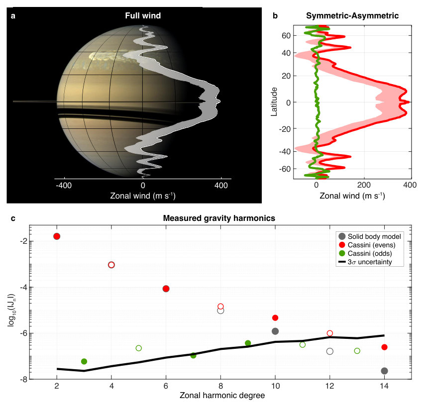 Figure 1
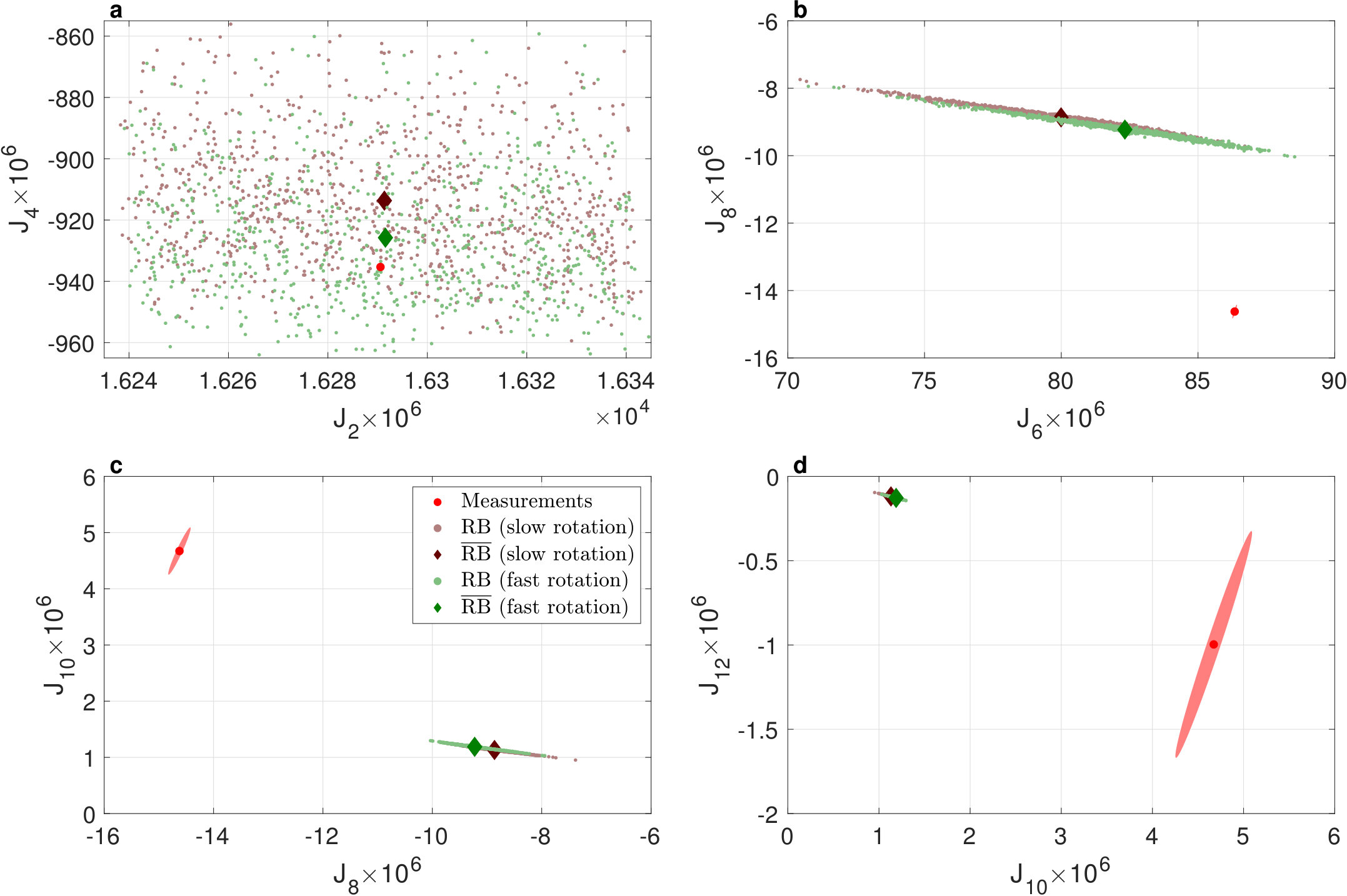 Figure 2
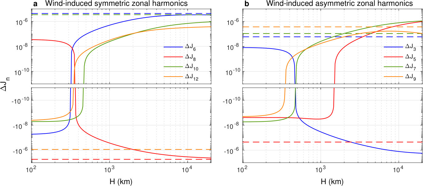 Figure 3
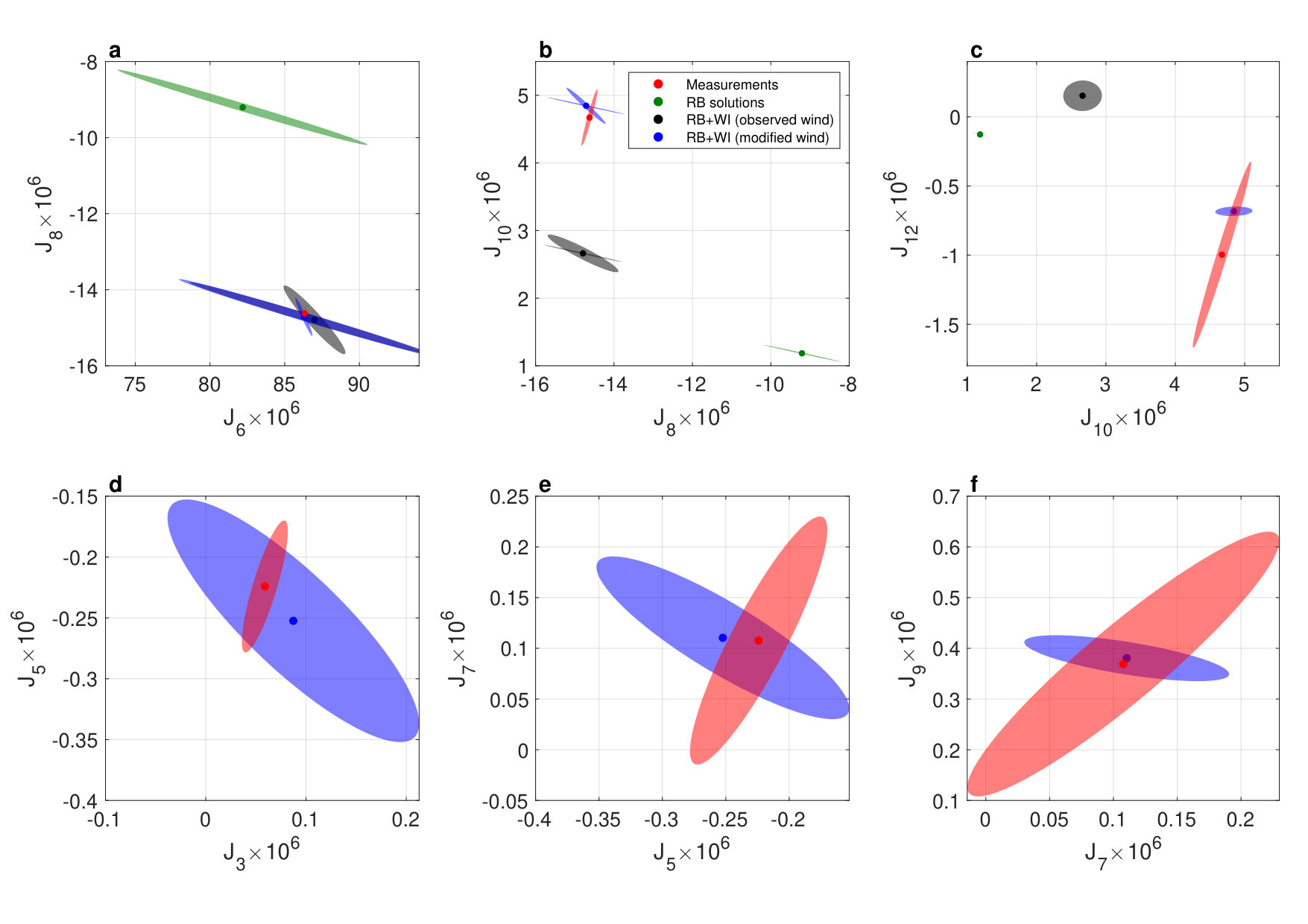 Figure 4
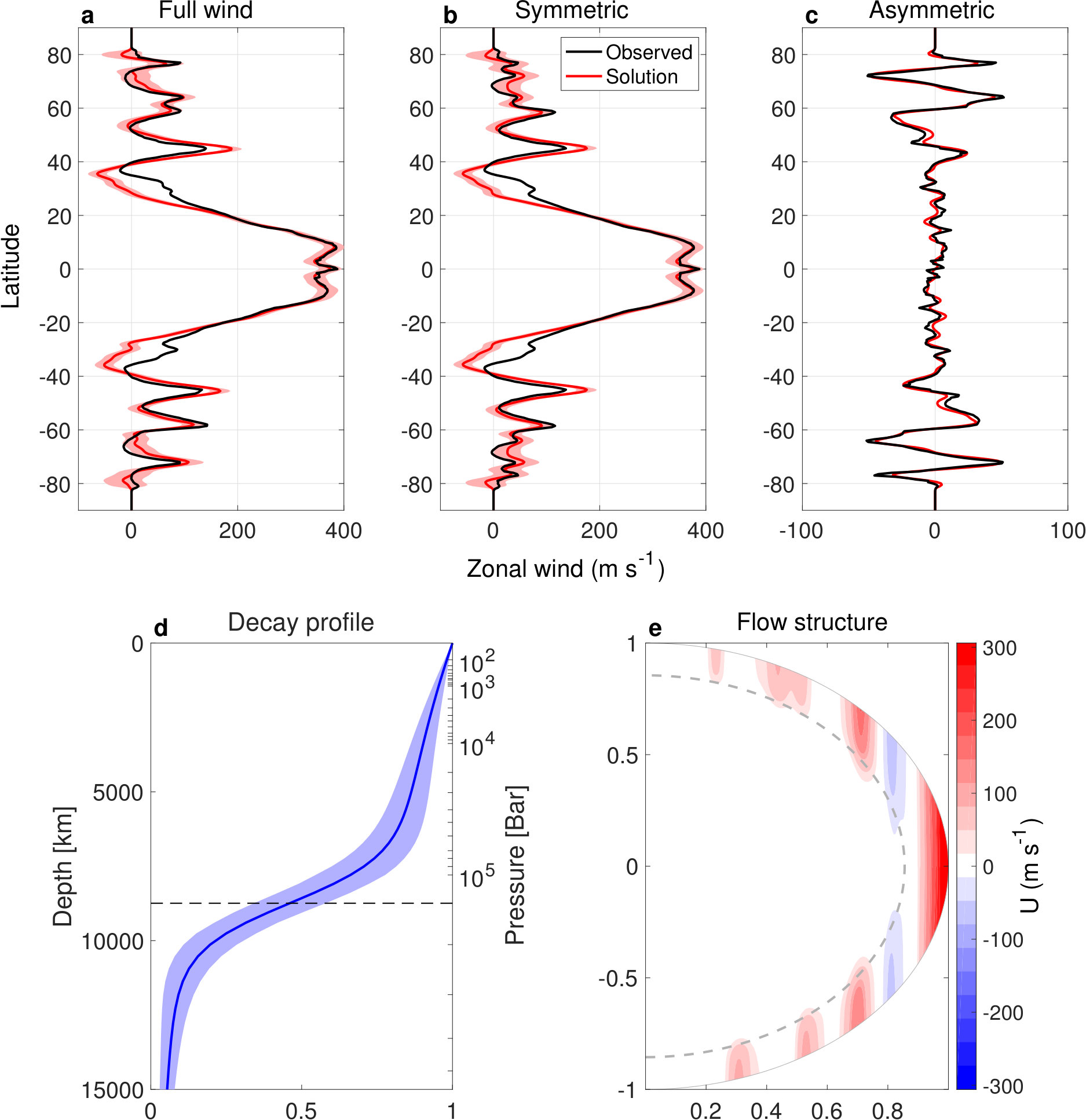 Figure 5
Peer Reviews
No public reviews on file for this paper yet. If you reviewed it on a platform where reviews are public (OpenReview, ICLR, NeurIPS, ICML), you can paste yours below so the community can read it here.
Videos
No videos yet. Explain this paper in a talk, walkthrough, or lecture? Add one.
Saturn’s deep atmospheric flows revealed by the Cassini Grand Finale
gravity measurements
Eli Galanti1, Yohai Kaspi1, Yamila Miguel2, Tristan Guillot3, Daniele Durante4, Paolo Racioppa4,
and Luciano Iess4
(Published in GRL: http://dx.doi.org/10.1029/2018GL078087)
Abstract
How deep do Saturn’s zonal winds penetrate below the cloud-level has been a decades-long question, with important implications not only for the atmospheric dynamics, but also for the interior density structure, composition, magnetic field and core mass. The Cassini Grand Finale gravity experiment enables answering this question for the first time, with the premise that the planet’s gravity harmonics are affected not only by the rigid body density structure but also by its flow field. Using a wide range of rigid body interior models and an adjoint based thermal wind balance, we calculate the optimal flow structure below the cloud-level and its depth. We find that with a wind profile, largely consistent with the observed winds, when extended to a depth of around km, all the gravity harmonics measured by Cassini are explained. This solution is in agreement with considerations of angular momentum conservation, and is consistent with magnetohydrodynamics constraints.
*1**Department of Earth and Planetary Sciences, Weizmann Institute of Science, Rehovot, Israel.
2Leiden Observatory, Leiden University, The Netherlands
3Observatoire de la Cote d’Azur, Nice, France
4Dipartimento di Ingegneria Meccanica e Aerospaziale, Sapienza Università di Roma, Rome, Italy*
1 Introduction
Whether the fluid below Saturn’s cloud levels is quiescent or exhibits strong zonal flows has been a long lasting open question. The zonal wind at the planet’s cloud-level is well established based on the Cassini measurements (Garcia-Melendo et al., 2011), with zonal flows that reach m s*-1* within a broad equatorial region, and a few narrower jets at higher latitudes (Fig. 1a, white line). The flow is predominantly north-south hemispherically symmetric (Fig. 1b, red line), with a much smaller asymmetric component that is more pronounced in the mid to high latitudes (Fig. 1b, green line).
However, aside from some observed variations in the wind strength between the upper and middle troposphere, there has been very little knowledge on the nature of the flow below the cloud-level. A possible answer was enabled by the gravity experiment conducted during the Grand Finale phase of NASA’s Cassini spacecraft (Iess et al., 2018). The measured gravity field (Fig. 1c, red and green dots) was found to be considerably different from that predicted by typical internal rigid-body models (gray dots), especially for gravity harmonics higher than . Initial estimates for the depth of the winds indicated very deep winds penetrating to a depth of more than km (Iess et al., 2018). This estimate, however, required a substantial modification of the meridional profile of the cloud-level winds and was determined by matching only the gravity harmonics and In addition, the background density profile used in the calculation of the wind-induced gravity harmonics was based on a specific interior model that might not represent all possible internal density structures.
was recently found that in Jupiter the part of the measured gravity field unaccounted for with rigid body models, can be attributed to a downward extension of Jupiter’s cloud-level winds to a depth of about km (Kaspi et al., 2018; Guillot et al., 2018). This motivates consideration of whether a similar procedure works for Saturn. While the flow inside a gas giant is expected to be aligned parallel to the axis of rotation due to angular momentum constraints (see Kaspi et al., 2018, for a detailed discussion), it is not clear whether this flow is well represented in the observed cloud-level winds. The observations of Saturn’s winds carry uncertainties that need to be taken into consideration (Garcia-Melendo et al., 2011). First, the sensitivity in the analyzed cloud-level winds reach at certain latitudes. Second, it was found that there exists a substantial wind shear between the wind at the upper ( mb) and middle ( mb) atmosphere, of up to at the equator and up to in the midlatitudes (Garcia-Melendo et al., 2011). A similar patten was also found using thermal wind balance (Fletcher et al., 2008), suggesting that the variations represent changes with depth of the large scale geostrophic flow. In addition, it was found that the flow exhibits variations in time of up to between the Voyager and Cassini observations. Therefore, it is possible that the flow structure in the depths relevant to the gravitational signal (thousands of kilometers deep) is somewhat different from that observed at the cloud level.
Another uncertainty in the determination of the cloud-level winds comes from of the need to calculate it with respect to the planet’s rotation rate, which is still not known with high certainty (Helled et al., 2015). The estimate of Garcia-Melendo et al. (2011) (Fig. 1a, white line) was done with respect to the Voyager rotation rate (Smith et al., 1982). More recent calculations (Anderson and Schubert, 2007; Read et al., 2009; Helled et al., 2015) show a faster rotation rate that shifts the winds to more negative values (Fig. 1a, gray area). Note that only the symmetric part of the wind is affected by the value of the rotation rate (Fig. 1b). This uncertainty was found to have an effect on the shape and density structure solutions of Saturn interior models (Helled and Guillot, 2013), and a substantial effect on the wind-induced gravity harmonic , while having only minor effect on the higher wind induced even harmonics (Galanti and Kaspi, 2017).
In this study we aim to decipher the flow structure that best explains all the gravity harmonics measured by Cassini in the gravity-dedicated Grand Finale orbits. Unlike Jupiter, where large odd harmonics were measured, in the case of Saturn we need to relay on the even harmonics, requiring the calculation of the contribution of Saturn’s rigid body to the gravity field. We thus use a wide range of rigid body (RB) models to map both the residual even gravity harmonics to be explained by the flow, and to determine the preferable background density profiles to be used in the calculation of the wind-induced (WI) gravity harmonics. Using a thermal wind balance, we find the top level zonal wind structure and its radial profile that best explain the measured gravity field. This methodology provides a rigorous and complete analysis of the gravity measurements.
The manuscript is organized as follows: in section 2 we explore the RB solutions for the gravity field. These solutions are then used to define the residual even gravity harmonics to be explained by the flow, which is analyzed using the WI solutions (section 3). Next, we include in the WI gravity calculation a search for a top level wind that allows the explanation of all measured gravity harmonics (section 4). We discuss the results and conclude in section 5.
2 The rigid body (RB) gravity field
In order to explore the range of gravity solutions consistent with the measurements we first construct interior models of Saturn that fit the observational constraints of Saturn’s radius and gravity harmonic , under the assumption that the interior of the planet rotates as a rigid body (RB) following the methodology of Guillot et al. (2018), which was effectively used for the analysis of Juno based Jupiter gravity field. Since is also affected by differential rotation (Galanti and Kaspi, 2017), we allow the RB solution to deviate from the measured value within the range , to cover a wide range of differential rotation scenarios corresponding to different rotation rates and depths of the zonal flows. (Galanti and Kaspi, 2017).
We assume a non-homogeneous structure for Saturn (e.g., Guillot, 1999; Fortney and Hubbard, 2003; Nettelmann et al., 2015; Vazan et al., 2016) with a possible diluted core scenario, as proposed recently for Jupiter (Wahl et al., 2017). The radial structure consists of 4 layers: (1) an and -poor atmosphere, (2) a metallic and -rich envelope, (3) a dilute core which is a metallic and -rich region with an increase in the heavy elements abundance, and (4) a core composed by ices or rocks. The diluted core (layer 3) is omitted in some of the models to allow exploration of both possibilities in Saturn interior. We assume an adiabatic interior, neglecting the effects of a non-adiabatic region on the gravitational harmonics, which are significantly smaller than the uncertainties discussed in this paper (Nettelmann et al., 2015). The outer boundary condition is set to at bar based on Voyager measurements (Lindal, 1992). The abundance of Helium in Saturn’s atmosphere is assumed to be (Helled and Guillot, 2013) and the value in the deeper layer is adjusted so that the overall Helium abundance corresponds to the assumed protosolar abundance of (Bahcall et al., 1995). The phase transition is set to occur at a pressure between and Mbar, in agreement with immiscibility calculations (Morales et al., 2013).
A crucial parameter in the modeling of the internal structures of giant planets is the equation of state (Hubbard and Militzer, 2016; Miguel et al., 2016). For and we use REOS3 (Becker et al., 2014) as well as MH13 (Militzer and Hubbard, 2013) that were derived using ab initio calculations, with some adjustments as detailed in Miguel et al. (2016). The heavy elements, composed by rocks and ices, are modeled using the equations of state for a mixture of silicates "dry sand" for rocks and "water" for ices (Lyon and Johnson, 1992).
In order to consider all possible interior structure configurations, some of the parameters that are poorly constrained were chosen randomly within a broad range (see supporting information). The simulations were performed with either a slow rotation rate (Smith et al., 1982) or a fast rotation rate (Helled et al., 2015). In total, a little over 1700 possible interior models for Saturn were calculated.
The gravitational harmonics are calculated using the theory of figures of 4th order (Zharkov and Trubitsyn, 1978; Nettelmann, 2017), combined with an integration of the recombined density structure in two-dimensions using a Gauss-Legendre quadrature (Guillot et al., 2018). This numerically efficient method allows the execution of the hundreds of calculations required. It has a known systematic bias compared to more detailed calculations made with a Concentric Maclaurin Spheroids method (Hubbard, 2012, 2013), therefore all gravity solutions presented here are corrected with , , , , and , calculated similarly to Guillot et al. (2018).
The range of RB solutions for the even gravity harmonics are shown in Fig. 2 for the slower rotation rate (brown dots) and the faster rotation rate (green dots), together with the measurements (red dots and ovals). Out of the 6 parameters defined above, the He transition depth has the largest effect on the solutions - larger transition pressure results in larger absolute values of for . Note that the parameters varied in the RB models affect mostly the deep interior structure of Saturn, hence and , and have a weaker effect on the atmosphere of Saturn, reflected in the higher even harmonics. As a result, the solution dispersion is large for and , and get smaller for higher harmonics. Note also that the fast rotation rate moves the solutions substantially toward the measurements, with larger absolute values in all harmonics.But most importantly, it is evident that while and can be explained entirely by the RB models (the measurements are well within the model uncertainties), the solutions for the higher harmonics, while closer to the measurements and having a much larger spread than the model used in Iess et al. (2018), cannot explain the measured values. The mean distance between the model solutions (brown and green diamonds) and the measured values (red dots) must to be the result of a wind-induced density anomalies.
3 The wind-induced (WI) gravity field
Given that Saturn is a large planet and a fast rotator, any large scale flow is governed by the thermal wind balance, relating the flow to the density field (Pedlosky, 1987; Kaspi et al., 2009). Assuming the flow is zonally symmetric and assuming sphericity (Galanti et al., 2017), the dynamical balance is between the flow gradient in the direction parallel to the axis of rotation and the meridional gradient of density perturbations
[TABLE]
where is the planet’s rotation rate, and are the rigid body density and gravity fields, is the flow field, is the anomalous density field, and and are the radial, latitudinal, and axis of rotation directions (see supporting information for a detailed derivation). This balance was used extensively to study the wind structure on Jupiter (e.g., Kaspi, 2013; Liu et al., 2013; Zhang et al., 2015; Kaspi et al., 2016; Galanti et al., 2017), as well as for the prediction of the wind-induced gravity field to be expected on Saturn (Kaspi, 2013; Galanti and Kaspi, 2017). The wind-induced (WI) gravity harmonics are calculated as the volume integral of projected onto Legendre polynomials
[TABLE]
where is the planetary mass, is the planet equatorial radius, and are the Legendre polynomials. For a detailed discussion of the method refer to Kaspi et al. (2018).
Following the same methodology used in Kaspi et al. (2018) we first assume the wind decays exponentially with a decay depth (see supporting information), and calculate the resulting gravity harmonics as function of (Fig. 3, solid lines). Given the mean values of the even harmonics of the RB model (Fig. 2, green diamonds), we can now plot the measured (Fig. 3a, dashed lines) in addition to the measured odd harmonics Fig. 3b, dashed lines), which are not affected by the RB solutions. Based on the observed cloud-level winds, this model is able to partially explain the even harmonics and , for which it asymptotically reaches the measured values of and , and about one third the value of , but cannot explain the odd harmonics. The WI solutions are found to be effected by the background density taken from the RB solutions - profiles with the highest densities in the outer layers () increase the value of the gravity harmonics by up to , compared to RB profiles with the lowest values.
We can then expend our search with a more complex decay function (see supporting information), looking for the optimal radial structure of the wind that gives the best fit the measured gravity harmonics. The optimal solution is found with , , and , where is the depth of a hyperbolic tangent and exponential radial profiles, is its width and is the ratio between the two functions. The resulting gravity harmonics for are shown in Fig. 4a,b,c as (black dots) along with the uncertainties associated with them (gray ovals). Also shown are the uncertainties associated with the RB solutions (additional gray ovals). As predicted with the simple model (Fig. 3), the optimal and are able to move the RB solution (green dots and ovals) in the direction of the measurements (red dots and ovals), with and explained within the uncertainties associated with the model, and being pushed half the way to the measurements. The odd harmonics remain inconsistent with the measurements and are outside the range presented in the figure. This implies that the observed cloud-level wind profile might not represent accurately the flow affecting the gravity field.
4 The wind below the cloud-level
The limited ability to explain all the measured when using the observed cloud-level wind suggests that the wind-induced gravity signal might be a result of a flow field that is somewhat different from that observed at the cloud-level. As discussed in section 1 this possibility has support in the observations, in which uncertainties in the analysis as well as variations in both time and depth are observed (Garcia-Melendo et al., 2011, Figs. 3 and 9). This implies that the search for a flow field that explains the measured gravity field requires an augmented optimization, one that would also allow the cloud-level wind itself to vary in addition to its radial decay profile. This can be achieved by decomposing the cloud-level wind into the first Legendre polynomials
[TABLE]
where are the coefficients defining the meridional wind solution. The optimization procedure for calculating is constructed to ensure that the deviation of the wind solution from the observed cloud-level wind is not larger then what is necessary to bring the gravity field solution within the uncertainty range of the measured field (see supporting information).
The optimal solution for the radial structure of the flow is found with , , and . The wind solution is shown in Fig. 5a-c (red lines), together with its uncertainty (red shading). Also shown is the observed cloud-level wind (black lines). In most latitudes the solution wind is very similar to the observed cloud-level wind and is well within the expected uncertainties discussed in Sec. 1). The largest deviations are around latitudes north and south, similar in location to the findings of Iess et al. (2018), but about half the size. The wind decay profile and the resulting flow structure (Fig. 5d-e) reveal that the wind behaves nearly barotropicly in the equatorial region (extending all the way to the equatorial plain in the direction of the spin axis), but nearly baroclinicly outside latitudes and , i.e. decaying before reaching the equatorial plain.
With the modified wind the WI model is able to fit all gravity harmonics taken into consideration (Fig. 4, blue dots and ovals), both the even and the odd harmonics. Importantly, the goal here is to have an overlap between the uncertainty of all the model gravity harmonics solutions (blue ovals) and the measurement uncertainties (red ovals). It would have been easy to get the model solutions (blue dots) to fit exactly the measurements (red dots), simply by relaxing the regularization of the winds (see supporting information), but with the cost of the wind solution getting farther away from the observations. By aiming for an overlap of the uncertainty ovals only, a balance is reached between the need for a viable solution and the need to keep the optimized winds as close as possible to the cloud-level observations.
5 Discussion and conclusion
The Cassini gravity measurements provide a unique opportunity to decipher the nature of the flow on Saturn. The initial analysis of Iess et al. (2018) pointed to the existence of deep flows in the equatorial region, yet these results were limited to a specific rigid body model, and as a result, required the surface wind to be substantially different from the observed cloud-level winds.
In this study we investigate the gravity field of Saturn, using a wide range of rigid body (RB) gravity models and a wind-induced gravity model in which the top-level wind is allowed to differ from the observed cloud-level wind. The RB solutions, while having a much broader range of solutions than those used in Iess et al. (2018), are still distinctively different from the measurement for all even harmonics higher than , therefore implying the existence of strong differential flows underneath the cloud-level. They also exhibit a considerable variance in the radial density structure, with higher densities in the outer layers associated with up to higher values of and , compared with the values obtained with the lower background density. These cases, explaining better the measurements, are mostly associated with a deeper transition depth (). Interestingly, these cases also allow the wind-induced gravity signal to match the measurements with less modification of the cloud-level wind, since both the RB and the WI solutions have higher values of and , thus pushing their sum farther toward the measurements.
With a conservatively modified cloud-level wind, extended to a depth of around km, all the relevant gravity harmonics can be explained, taking into account the associated uncertainties in both the measurements and the model solutions. In most latitudes the optimal top level wind is similar to the observed wind, with the largest deviations found around latitudes north and south, similar to the deviation found by Iess et al. (2018) but twice as small. This is a result of the different SB background density and gravity harmonics solutions used here, as discussed above. In order to explain the measured odd harmonics, the modifications needed in the asymmetric flow are minor and are well within the uncertainty in the cloud-level wind observations.
The optimal flow depth of km is consistent with estimates of the depth in which the conductivity of the fluid prohibit strong flows (Liu et al., 2008; Cao and Stevenson, 2017). Interestingly, this depth, taken at the equator, is approximately the location where the cylindrical flow outcropping at is, and where the flow is found to be most different from that observed at the cloud-level. Investigating this circumstantial result might require the analysis of a dynamical model in which magnetohydrodynamical considerations are included (Galanti et al., 2017).
Acknowledgments: EG and YK acknowledge support from the Israeli Space Agency and from the Helen Kimmel Center for Planetary Science at the Weizmann Institute of Science. DD, PR, and LI were supported by the Italian Space Agency. The data plotted in the figures is available at https://www.dropbox.com/sh/enef9c2z1lb5x1s/AAByea2T9Cx-oqtLYOfuvCjsa?dl=0.
The reference list from the paper itself. Each links out to its DOI / PubMed record.
- 1Anderson and Schubert (2007) Anderson, J. D., and G. Schubert (2007), Saturn’s gravitational field, internal rotation, and interior structure, Science , 317 , 1384–1387.
- 2Bahcall et al. (1995) Bahcall, J. N., M. H. Pinsonneault, and G. J. Wasserburg (1995), Solar models with helium and heavy-element diffusion, Rev. Mod. Phys. , 67 , 781–808.
- 3Becker et al. (2014) Becker, A., W. Lorenzen, J. Fortney, N. Nettelmann, M.Schattler, and R. Redmer (2014), Ab initio equations of state for hydrogen (h-reos.3) and helium (he-reos.3) and their implications for the interior of brown dwarfs, The Astrophysical Journal Supplement Series , 215 (2), 21.
- 4Cao and Stevenson (2017) Cao, H., and D. Stevenson (2017), Zonal flow magnetic field interaction in the semi-conducting region of giant planets, Icarus , 296 , 59–72.
- 5Fletcher et al. (2008) Fletcher, L., P. Irwin, G. Orton, N. Teanby, R. Achterberg, G. Bjoraker, P. Read, A. Simon-Miller, C. Howett, R. de Kok, et al. (2008), Temperature and composition of Saturn’s polar hot spots and hexagon, Science , 319 (5859), 79–81.
- 6Fortney and Hubbard (2003) Fortney, J. J., and W. B. Hubbard (2003), Phase separation in giant planets: inhomogeneous evolution of saturn, ica , 164 , 228–243.
- 7Galanti and Kaspi (2017) Galanti, E., and Y. Kaspi (2017), Prediction for the flow-induced gravity field of Saturn: implications for Cassini’s Grand Finale, Astrophys. J. Let. , 843 (2), L 25.
- 8Galanti et al. (2017) Galanti, E., Y. Kaspi, and E. Tziperman (2017), A full, self-consistent treatment of thermal wind balance on oblate fluid planets, J. Fluid Mech. , 810 , 175–195.