Frustration effects at finite temperature in the half filled Hubbard model
Gour Jana, Anamitra Mukherjee

TL;DR
This paper explores how frustration introduced by next nearest neighbor hopping affects the finite temperature phases of the half filled Hubbard model, revealing a pseudogapped phase and its properties.
Contribution
It demonstrates the emergence of a frustration-driven pseudogapped phase at finite temperature and maps its crossover to metallic and insulating states, supported by semiclassical and exact diagonalization methods.
Findings
Introduction of $t'$ creates a finite temperature pseudogap phase.
Resistivity deviates from quadratic temperature dependence in the pseudogap phase.
Exact diagonalization indicates a frustration-driven pseudogap at zero temperature.
Abstract
We investigate the finite temperature properties of the half filled Hubbard model in two dimensions, with onsite interaction (), in presence of (frustrating) next nearest neighbor hopping () using a semiclassical approximation scheme. We show that introduction of results in a finite temperature pseudogapped (PG) phase that separates the small Fermi liquid and large Mott insulator. We map out the PG to normal metal crossover temperature scale () as a function of and . We demonstrate that in the PG phase, the quadratic dependence of resistivity on temperature is violated due to thermally induced spin fluctuations. We conclude with exact diagonalization calculations, that complement our finite temperature results, and indicate the presence of a frustration driven PG state between the Fermi liquid and the Mott insulator at zero…
Click any figure to enlarge with its caption.
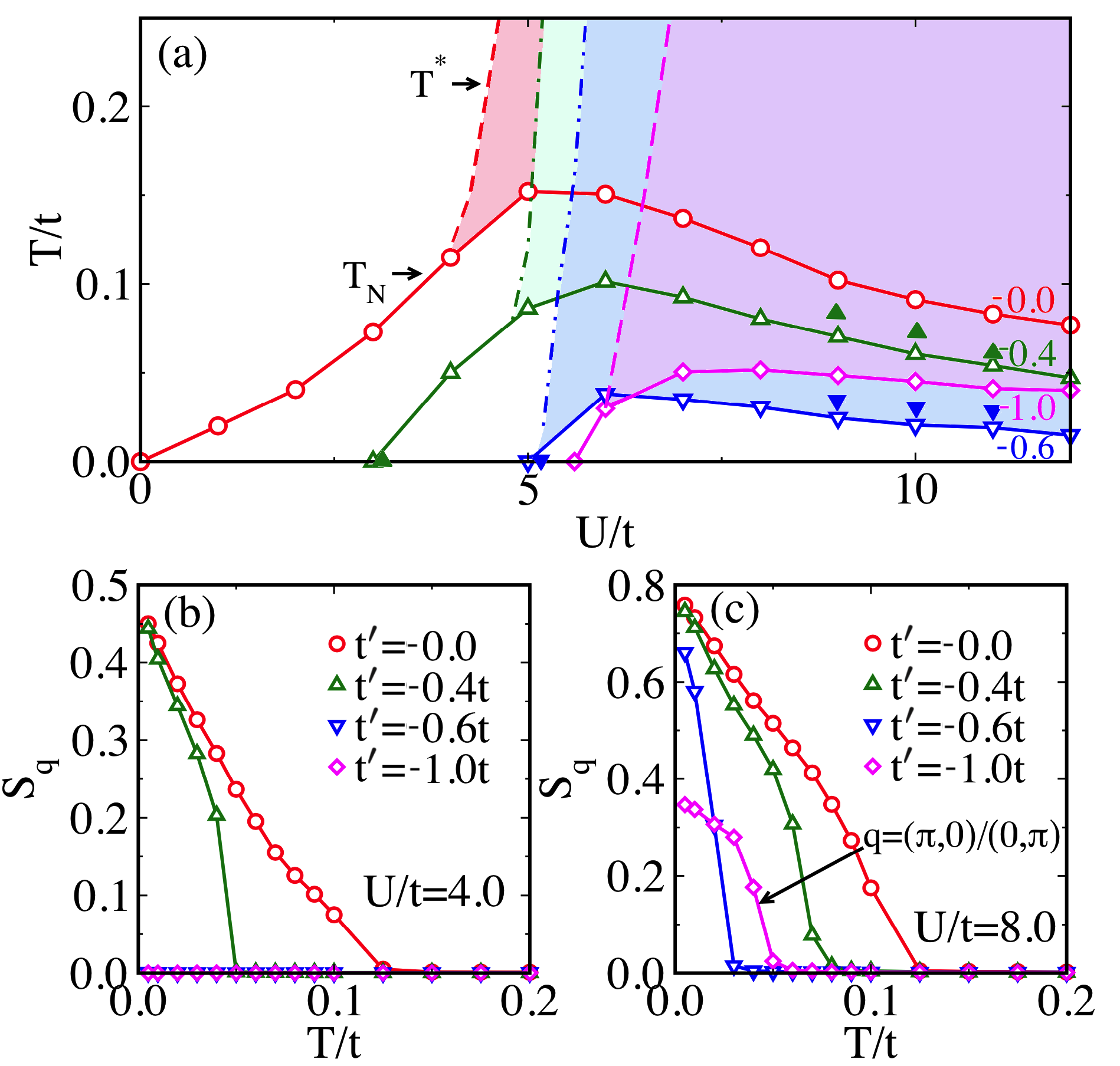 Figure 1
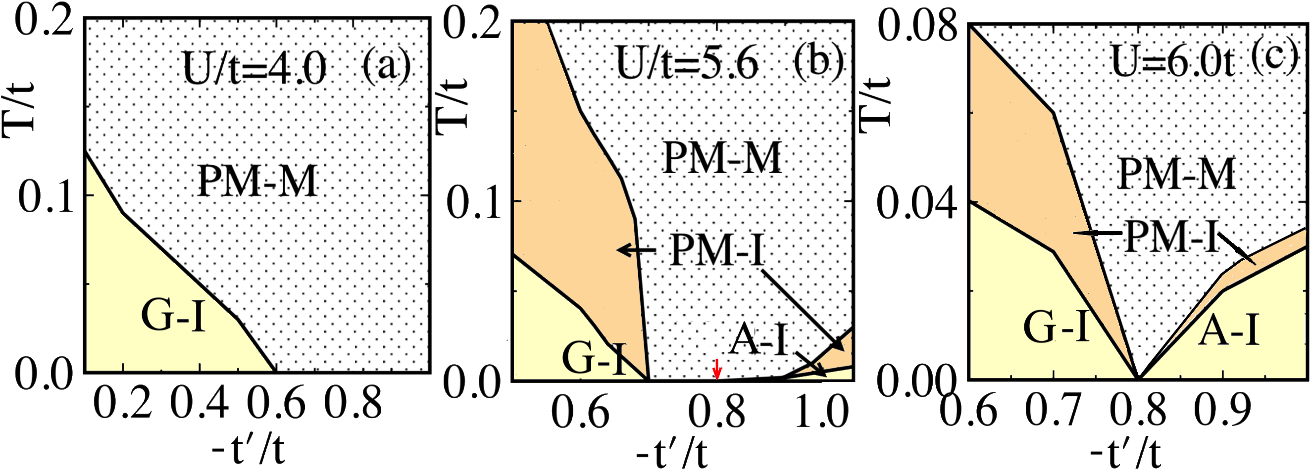 Figure 2
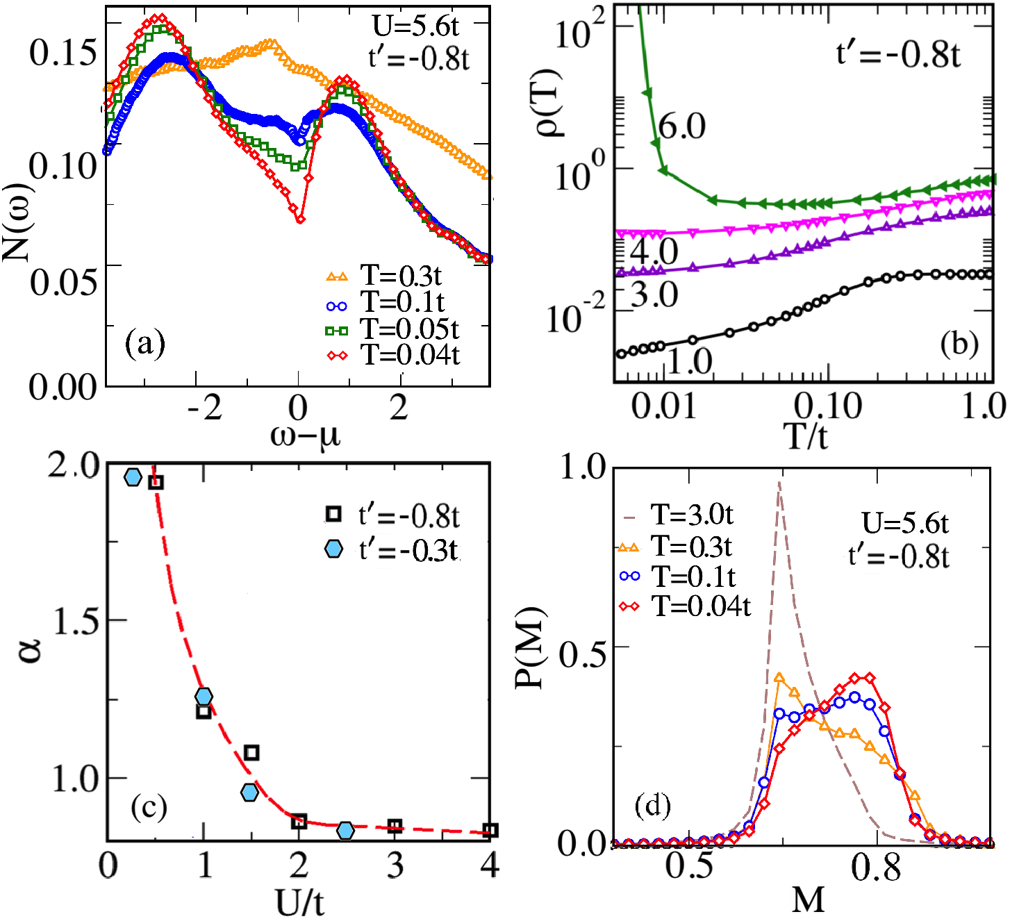 Figure 3
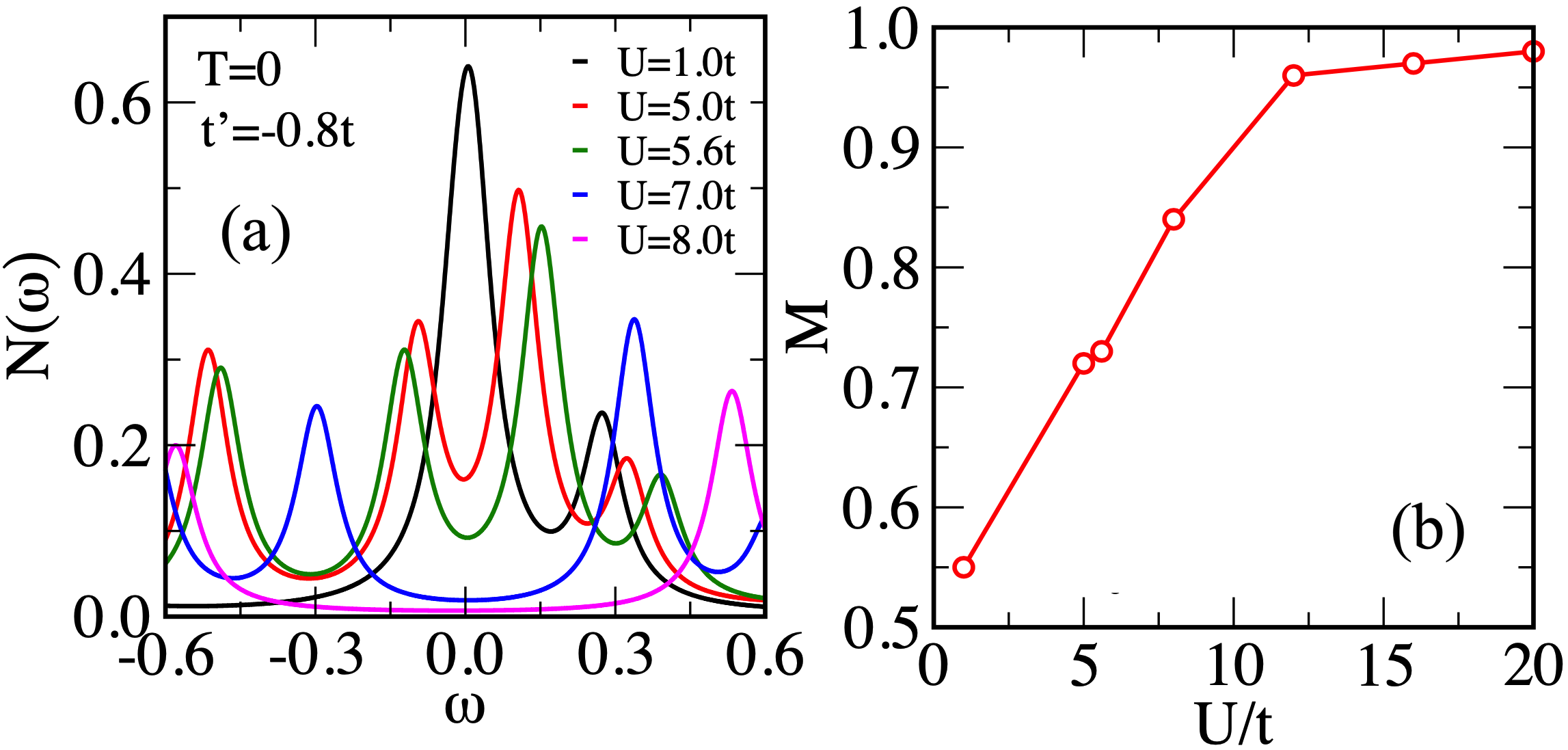 Figure 4
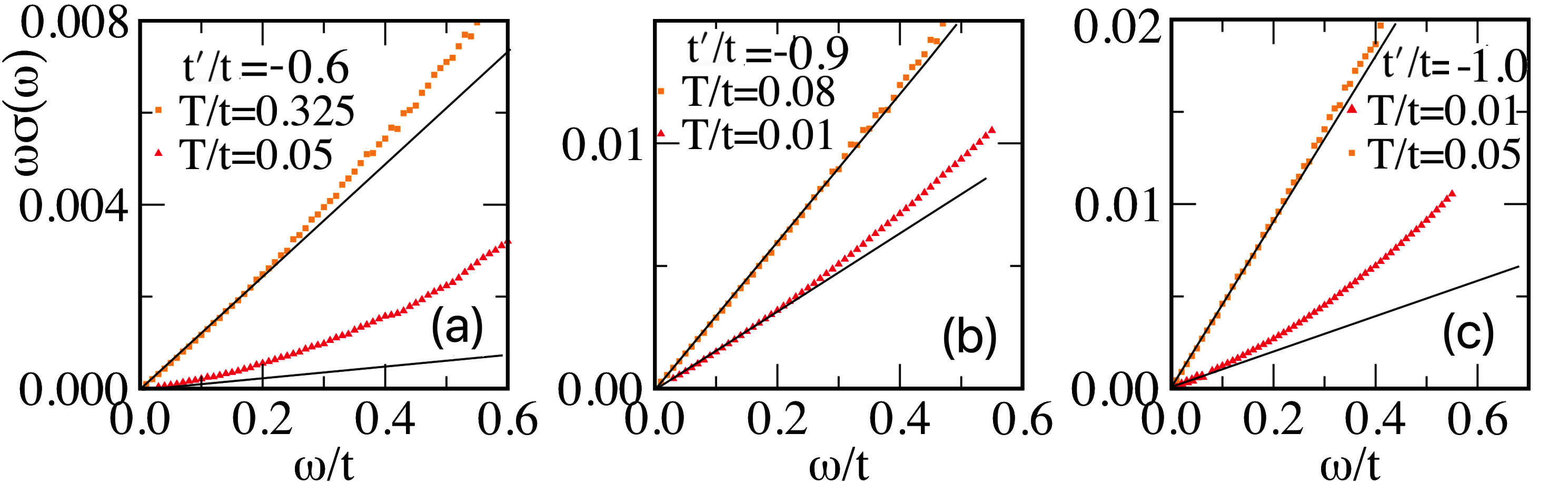 Figure 5
Peer Reviews
No public reviews on file for this paper yet. If you reviewed it on a platform where reviews are public (OpenReview, ICLR, NeurIPS, ICML), you can paste yours below so the community can read it here.
Videos
No videos yet. Explain this paper in a talk, walkthrough, or lecture? Add one.
Frustration effects at finite temperature in the half filled Hubbard model
Gour Jana
Anamitra Mukherjee
School of Physical Sciences, National Institute of Science Education and Research, HBNI, Jatni 752050, India.
Abstract
We investigate the finite temperature properties of the half filled Hubbard model in two dimensions, with onsite interaction (), in presence of (frustrating) next nearest neighbor hopping () using a semiclassical approximation scheme. We show that introduction of results in a finite temperature pseudogapped (PG) phase that separates the small Fermi liquid and large Mott insulator. We map out the PG to normal metal crossover temperature scale () as a function of and . We demonstrate that in the PG phase, the quadratic dependence of resistivity on temperature is violated due to thermally induced spin fluctuations. We conclude with exact diagonalization calculations, that complement our finite temperature results, and indicate the presence of a frustration driven PG state between the Fermi liquid and the Mott insulator at zero temperature as well.
I Introduction
One of the fundamental questions in strongly correlated systems is the fate of a Fermi liquid (FL) under strong correlation and frustration effects. Intimately tied to this, are the understanding of important issues in materials theory such as, the pseudogapped phase in the doped cuprates Dagotto (1994); Plakida (2006), non Fermi liquid (n-FL) behavior in the the heavy fermion compoundsColeman et al. (2001); Miranda and Dobrosavljevic (2005) and rare earth nickelates Mikheev et al. (2015); Liu et al. (2013); Phanindra et al. (2018). With these questions in mind, the Hubbard model, with nearest () and next nearest hopping () and its variants, have continued to be in focus of intense investigations, using a host of approaches such as Hartree-Fock mean field theory Lin and Hirsch (1987a); Kondo and Moriya (1996); Yu and Yin (2010); Raczkowski et al. ; Langmann and Wallin (2007); Nevidomskyy et al. (2008); Yamaki et al. (2013) quantum Monte-Carlo Huang et al. (2001); Lin and Hirsch (1987b); Husslein et al. (1996); Langmann and Wallin (2007); Duffy and Moreo (1997), variational methods Becca et al. (2009), Gutzwiller projected wave-function approach Tocchio et al. (2008); Capello et al. (2005), slave boson theory Yang et al. (2000), dynamical mean field theories Chitra and Kotliar (1999); Gull et al. (2009); Hofstetter and Vollhardt ; Werner et al. (2009); Ferrero et al. (2009); Liebsch et al. (2008) and effective spin models at large Hu and Wang (2016); Jiang et al. (2012); Isaev et al. (2009); Darradi et al. (2008); Delannoy et al. (2009). Further, lattice implementation of time dependent density functional theory has also been used to study effect of disorder induced frustration on transportVettchinkina et al. (2013) and melting of Mott phase Kartsev et al. (2013) in the Hubbard model.
It is well established that the Slater insulating state at half filling and weak interaction strength (), is destabilized due to particle hole symmetry breaking for any non zero and results in a FL metal. Upon increasing , this metal undergoes a Mott transition with either () or ()/(0,) magnetic order depending on the strength of the next nearest hopping . The investigation of induced metallic state at zero temperature using dynamical cluster approximation (DCA) in the paramagnetic phase Gull et al. (2009); Werner et al. (2009) and cluster-dynamical mean field theory (CDMFT) Ferrero et al. (2009); Liebsch et al. (2008) have lead to the following major conclusions. For small , increasing causes the metal to undergo a two stage transition. Instead of directly going from a metal to a Mott insulator, there is an intermediate regime where the Fermi surface is gapped out along the () and () directions, while the () direction remains gapless. The total density of states (DOS) shows a pseudogap and the metal is predicted to be a n-FL. Further, renormalization group studies Halboth and Metzner (2000a); Hankevych et al. (2002); Halboth and Metzner (2000b) suggest possible tetragonal or rotation symmetry breaking of the Fermi surface, as has also been found in the studies of the model Edegger et al. (2006); Yamase and Kohno (2000a, b). In spite of these important advances, there are a very few results on finite temperature propertiesFratino et al. (2017) and nature of the metallic state stabilized by frustrationGull et al. (2009); Werner et al. (2009). Both (CDMFT)Fratino et al. (2017) and (DCA)Gull et al. (2009); Werner et al. (2009) assume a paramagnetic background and suffer from well known analytic continuation issues (as they are typically formulated in imaginary time). Thus, the role of magnetic background and impact of temperature has remains inadequately understood.
Solving the Hubbard model without particle-hole symmetry using standard DQMC approach is limited to high temperatures due to fermion sign problem. Further in DQMC sampling over the imaginary time and spatial coordinates with good accuracy is numerically extremely prohibitive. In addition analytic continuation issues for extracting real frequency quantities like density of states are well known. Given the rather challenging nature of the problem, in the present paper we employ a recently developed semiclassical Monte-Carlo (s-MC) that is free of fermion sign problem and is computationally inexpensive, allowing access to large system sizes. Being semi-classical in nature, the approximation agrees well with DQMC in the thermally dominated phase and has been studied and compared against DQMC in our previous publication Mukherjee et al. (2014, 2015a) for the square lattice Hubbard model at half filling. Given this background, it is natural to test the method to extract finite temperature properties of the rather difficult Hubbard model in two dimensions. Also, while previous studies have heavily focussed to , a value relevant for the cuprates, here we study the effect of frustration for the entire window of .
We begin by summarizing our main results. We first discuss the impact of frustration on the magnetic phases at finite temperatures. This includes, suppression of the , G-type magnetic transition temperature, shifting of the regime of preformed local moments to larger values and emergence of A-type ( or ) order at large frustration. We then present the metal insulator phase diagrams at different values to establish the existence of finite temperature PG metal and determine the temperature scale () for the PG to normal metal crossover. From the dependence of resistivity on temperature, we show a continuous crossover from a small Fermi liquid (FL) to the PG phase (with the resistivity temperature exponent deviating strongly from 2). We show how the interplay of frustration and correlation drives local moment fluctuation at finite temperature and stabilizes the PG metal in the passage from the FL to a Mott state. We close by providing ED results, that establishes the same phenomenology of a PG state punctuating the FL to Mott transition with increasing interaction strength, in presence of frustration in agreement with DCA resultsGull et al. (2009); Werner et al. (2009).
The paper is organized as follows. In Sec. II we briefly discuss effective Hamiltonian derived from the many body problem. In Sect. III we present our main results and conclude the paper in Sec. IV.
II Model method
The Hubbard model has the following form:
[TABLE]
Here the model is defined on the two dimensional square lattice with being the nearest neighbour hopping and being the next nearest neighbor hopping. is the correlation strength and and denote the kinetic and interaction Hamiltonians respectively.
The (s-MC) approachMukherjee et al. (2014, 2015a), is based on Hubbard-Stratonovich (HS) decomposition of the interaction Hamiltonian by introducing auxiliary fields (Aux. F.) just as in Determinantal Quantum Monte Carlo (DQMC). To apply the Hubbard Stratonovich (HS) decomposition, we first write the local interaction term as a sum of squares of total on-site density and spin operator. In the Appendix subsection A, we provide detailed derivation of the effective one body Hamiltonian (), that is obtained from the many body problem after employing HS transformation and retaining only the temperature induced spatial fluctuations of the (Aux. F.)s. For continuity of the main paper, we mention that two (Aux. F.) are introduced, a vector field and a scalar field at every site of the lattice . They couple to the spin and the charge degrees of freedom respectively. With the introduction of these fields, as shown in the Appendix, we get the following effective Hamiltonian, which is used in the paper:
[TABLE]
Here, denote the three Pauli matrices and are related to the spin operator at a site by , as discussed in Appendix A. We confine our calculations to the regime of , to compare with cuprate inspired literature that have chosen . We will measure all energy scales in units of the nearest neighbour hopping . We note that the effective Hamiltonian looks identical to a simple (mean field) Hartree Fock model. The crucial difference of (s-MC) from a finite mean field theory is that, the Aux. F. appearing in are treated within a classical Monte Carlo instead of using self consistency or saddle point approach, as would be done in a mean field treatment. The thermal sampling brings in the effects of spatially inhomogeneous thermal fluctuations. These thermal fluctuations capture many of the well established features such as the regime of preformed local moments, non-monotonic dependence of on as found in DQMC in the unfrustrated problemMukherjee et al. (2014). These results cannot be produced in an unrestricted finite Hartree-Fock mean field theory. However, at low temperatures, when quantum fluctuations dominate, the s-MC reduces to a uniform Aux. F. solution identical to Hartree-Fock mean field theory as the temporal (quantum) fluctuations of the Aux. F. is not taken into account. This limits the validity of the s-MC only to thermally dominated regime.
The calculation scheme for s-MC is the following. At any fixed temperature, the goal of the s-MC is to generate equilibrium configurations of Aux. F. through a Monte Carlo scheme. The coupled one body quantum problem is exactly diagonalized for a fixed Aux. F. background and the total free energy is used to update the Aux. F. within a Metropolis algorithm. The method of classical Monte-Carlo coupled with exact diagonalization used to solve Eq. 2 is detailed in Appendix subsection B. Here we, very briefly, outline some relevant details. We start by choosing a background configuration of (Aux. F.) at a high temperature, then diagonalize the system in that (Aux. F.) background. We then update the (Aux. F.), re-diagonalize the coupled fermion problem. The free energy difference is used to accept the (Aux. F.) update. After adequate thermalization system sweeps (involving update attempts by visiting each site sequentially), we generate equilibrium configurations of (Aux. F.) from which observables are calculated. As in classical Monte-Carlo, we typically anneal down from high to low temperatures. A number of indicators were calculated, density of states (DOS) , static spin structure factor , optical conductivity and quantum local moment distribution . The definitions of these standard indicators are given in the Appendix subsection C. Computational codes for (s-MC) were developed in house.
III Results
1. Evolution of magnetic phases with temperature:
We discuss the phase diagram, showing the magnetic phases for different values in Fig. 1 (a). Before proceeding we make the following important cautionary note. The Mermin-Wagner theorem states that in 1D or 2D systems with SU(2) invariant Hamiltonian with short range spin interactions, magnetic ordering scale tends to zero at any finite temperature in the thermodynamic limit. Given this, the magnetic transition temperatures quoted in the present paper should be understood as crossover temperature scales at which the magnetic spin-spin correlation length extends over the system size.
The for q or G type antiferromagnetic order at , is shown by the solid red line with circles in panel (a). For , we see the expected non monotonic behavior of with . The dashed (red) line demarcates the crossover between the preformed local moment regime with pseudogapped DOS for and paramagnetic metal for . The preformed local moment extends over the entire region between the red dashed line and the curve. The case, studied by us previously, shows that the s-MC approach goes much beyond simple finite temperature Hartree-Fock calculations and can capture the scaling of at large and the existence of the preformed local moment state above . For detailed results on temperature dependence of specific heat, local moments, double occupation as well as solution of the model on very large lattices (2562) in 2D and () in 3D, we refer to our earlier workMukherjee et al. (2014, 2015a).
With increasing magnitude of , the frustration increases. We find that this causes an an overall suppression of for G type magnetic order and the shifts the regime of preformed local moment (broken line of same color) to higher values. We find that within numerical accuracy, the G type magnetic order is suppressed to zero, for . Beyond , there is an emergence of A type antiferromagnetic order. Typical data for A type antiferromagnetic order (magenta diamonds) and the corresponding (magenta dashed line) are shown for in panel (a). We also show data for three dimensional 83 systems with solid symbols for (solid up triangles) and (solid down triangles) at large , to show the qualitative correctness of 2D calculations.
Panels (b) and (c) show supporting magnetic structure factor data. The magnetic structure factors for in Fig. 1 (b) shows the gradual suppression of the q magnetic order with increasing , eventually leading to a paramagnet (PM). In panel (c), we see that at the suppression in the q order and an eventual formation of q or order with increasing magnitude of . The regime of preformed local moments for , at finite , is discussed next.
2. Finite phases in presence of frustration:
To extract the impact of frustration of the thermal evolution of insulating states, in Fig 2 (a) to (c) to show the phase diagrams at three valueslow . The plots are shown for increasing values of . While for , the ground state of all the three cases are insulating antiferromagnets, we find strikingly different thermal response in presence of frustration. As discussed below, these phase diagram bring out the contrasting effect of frustration on weak and strong correlation situations.
The finite scale for metallization of the insulating states are determined by studying the behavior of the optical conductivity () with . For a metal there has to be a constant DOS close to the Fermi energy. Thus, should have a linear dependence on as . For (charge gapped) insulator there is typically a gap in up to some finite frequency starting from . The details of the optical conductivity calculations are discussed in the Appendix subsection D. Here we focus on the main results.
We find that at smaller values, the temperature scale for metallisation of the G type Mott insulator is monotonically suppressed with increasing . The G type magnetic order is also lost simultaneously with loss of the insulating nature. The non magnetic metal remains stable all the way up to the maximum possible value of frustration () and is devoid of local moments except for very small frustration values. In sharp contrast, on increasing , in panel (b), correlation effects conspire with frustration to form a new Mott state with A type magnetic order, which is most stable for (with the largest metallisation temperature scale as seen in panel (b)). This A type insulator invades the metallic regime, essentially limiting the metal to finite regime at low and fanning out with increasing temperature. With further increase in , in panel (c), the metallic regime shrinks to a point at (within numerical accuracy).
With temperature increase, for the larger cases in panels (b) and (c), the antiferromagnetic insulator first gives way to a PM insulator and then to a PM-M. This is because at larger , local moments form at a temperature higher that the magnetic ordering scale. Although we do not report it here, we find a two peak specific heat structure one corresponding to the moment formation and the other to moment ordering temperature, similar to the unfrustrated caseMukherjee et al. (2014). The effect of local moments on the nature and transport properties of the metal at finite temperature is discussed next.
3. Pseudogapped metal at finite :
We now we focus on the behavior of the frustration induced metal at finite temperature. We would like to emphasize that the (s-MC) method can provide reliable results in thermally dominated regime. At low temperatures, where quantum fluctuations are important, it reduces to inhomogeneous Hartree-Fock. Thus in this section we provide the s-MC results and discuss results from exact diagonalization in the next section. For demonstration, we show data at and . This point is marked in by the small red arrow in Fig. 2 (b).
Fig. 3 (a) shows the DOS at different temperatures for this metallic state. We see that, the non-pseudogapped DOS at very high temperature (orange curve with triangles) develops a PG with temperature decrease. Further, the PG deepens with reducing temperature. For this value of , thus the DOS are shown for , where thermal fluctuations dominate. Such pseudogap feature is seen for the entire metallic regime at and in Fig. 2 (b) and (c) respectively. For , the PG is restricted to small values. Panel (b) in Fig. 3 shows the resistivity as a function of temperature at and different values. We see a transition from an insulator for to a metal for . The scales in Fig. 1 (a) are defined to be the highest temperature () where the DOS develops a local minima at .
Panel (c) shows the exponent of the temperature dependence of , obtained from fitting resistivity for the metallic casesran for (open squares) and for (filled hexagons). We see that , only for small values. Beyond , there is a sharp drop in the value of the exponent, and it saturates to a sub linear value. continues to be remain fixed at the sub linear value till the Mott state is reached at for and at for .
To investigate the cause of the deviation of from 2, in panel (d) we show the real space distribution of local spin moments, with decreasing . The data is shown at and that is close to the Mott insulator at . Here , which is equivalent to at half filling. Thus, the value implies no local moments, as for . For the high temperature case, the DOS is non-pseudogapped and the has a dominant peak at around 0.5 (brown dashed line) indicating almost no local moments. Where as in the pseudogapped regime, the is highly non uniform. This indicates that once local moments start forming in the vicinity of the Mott state, frustration makes their spatial distribution non uniform. The ensuing scattering of the fermions from these spatially fluctuating moments causes the deviation from the FL behavior for the resistivity. As temperature is lowered further, we see that the moment distribution in real space begins to peak at about . As , this peak is expected to grow and become uniform, which would be the Hartree-Fock result. In this limit the s-MC method will show a non-pseudogapped state. Thus, as temperature is lowered if the PG is to survive the theory needs to incorporate quantum fluctuations. For this we turn to the limit in the next section. We also note that similar deviation of and pseudogap occurs near the metal to Mott insulator boundary for all . Values of for small are shown by filled hexagons in Fig. 3 (c). For this case the Mott state occurs beyond . For , it is difficult to numerically claim a PG phase.
4. Pseudogapped metal at :
So far we have established the existence of a finite PG metal and its origin has been shown to be spatial fluctuations of local moment. As mentioned above, it is expected that at low , quantum fluctuations will dominate. In this regime s-MC produces uniform moment static solutions, which can not host a pseudogapped state. In Fig. 4 we present Lanczos based ED density of states in panel (a) and evolution of local moment size in panel (b) on small () clusters. The data is shown for and different values. We see that the (normal) non-PG DOS at small , develops a pseudogap for to . In this range, the local moment size grows from 0.5 (uncorrelated value) to . This shows a clear correlation between existence intermediate sized local moment and the pseudogapped state at . The PG eventually hardens in to a Mott gap once the moment size grows beyond . This quantum fluctuation driven PG crosses over to the s-MC thermal fluctuation induced PG. This large result complements previous results at small valuesGull et al. (2009); Werner et al. (2009).
IV Conclusions Discussion
In this paper we have used a semiclassical-Monte-Carlo approach to study the effects of correlation and frustration in the two dimensional Hubbard model at half filling at finite temperature. We have studied finite evolution of magnetic phases, metal insulator transitions and have mapped out the temperature scale () of the crossover of the PG regime to normal metal. Our finite temperature s-MC and Lanczos results are consistent and show that the Fermi liquid to Mott transition with increasing , in presence of intermediate to large frustration (), is not a direct transition, but goes through a pseudogapped metallic phase phase. While we have focussed at , we have found numerically that this phenomenology holds for a between -0.2 to -1.
As mentioned in the paper, the goal of the s-MC method is to generate equilibrium configurations of Aux. F. through a classical Monte Carlo at given temperature. The acceptance of an attempted update of Aux. F. depends on both the existing classical Aux. F. background as well as the quantum mechanical fermion problem. Away from the metal insulator boundary, we find uniform Aux. F. configurations minimize the free energy leading to a small uniform Fermi liquid metal or a large Mott state with spatially uniform local moments. At finite temperature, and close to the phase transition, the Aux. F.s access free energy minima corresponding to the Fermi liquid and the Mott insulator due to thermal fluctuations and stabilize inhomogeneous local moments which scatter against fermions leading to the finite temperature pseudogapped state. At very high temperature (), the Aux. F. decouple from the fermions, as was demonstrated in our earlier work on the unfrustrated Hubbard modelMukherjee et al. (2014), and the pseudogapped state disappears. The method works well in this intermediate to high temperature regime where thermal fluctuations dominate the physics. At sufficiently low temperature as it misses out on quantum fluctuations and reduces to inhomogeneous Hartree-Fock limit. The determination of the thermal to quantum fluctuation dominated crossover as a function of temperature is, at present, an open question. Due to this our strategy is to provide complementary Lanczos results that, within size limitations, indicate frustration driven pseudogapped state between the Fermi liquid and the Mott insulator.
In conclusion, these results contribute to the long standing questions of the nature of strong interaction driven metal-insulator transitions in the background of frustration and are of relevance to many body theory and materials physics alike.
.
V Acknowledgement
We acknowledge the KALINGA, NOETHER and XANADU computational clusters at NISER. We also acknowledge, Nitin Kaushal for helping set up the ED code.
APPENDIX
In the subsection A we discuss the derivation of the used in the main paper. In subsection B we present the technical details of solution methodology and in subsection C, we define the various indicators used to study the effective Hamiltonian.
V.1 Derivation of
[TABLE]
Here, the spin operator is , , are the Pauli matrices, and is an arbitrary unit vector. In the previous identity, we have used the fact that . This rotation invariant decoupling results in the correct Hartree-Fock saddle point after implementing a Hubbard-Stratonovich (HS) decomposition. We start with the partition function where the trace is over all particle numbers and site occupations. , with set to 1. We divide the interval into equally spaced slices, defined by , separated by and labeled from 1 to . For large M, we employ the usual Suzuki-Trotter decomposition, to write to first order in . From Eq. (2) and the HS identity, , for any time slice , is found to be proportional to,
[TABLE]
Here two auxiliary fields, that couples to the local charge density, and that couples to the spin density are introduced. Defining the product as a new vector auxiliary field, at every site we can write the partition function as:
[TABLE]
The integrals are over the auxiliary fields, at every site and the argument denotes imaginary time slice label. The product over from M to 1 implies time ordered products over time slices, with the earlier times appearing to the right. Finally, the in the integral, implies integration over the amplitude and orientation of vector auxiliary fields, .Dropping the dependence of (Aux. F.) allows us to extract an effective Hamiltonian from . To make a further simplification to treat the Aux. field at its saddle point. While this is not necessary, it reduces the number of Aux. fields to be handled per site and leads to efficient computation. Thus in the effective Hamiltonian () the fermions couple to the ‘static’ HS field and to the average local charge density. With the redefinition we can finally write the effective Hamiltonian as:
[TABLE]
V.2 Solution of
coincides with the mean-field Hamiltonian at , where has the interpretation of the local magnetization. However at finite temperature these (Aux. F.) do not play the role of magnetization and should be thought simply as some classical variables (as we have dropped the dependence) which can take arbitrary amplitude and angular fluctuations.
We simulate by sampling the fields within a classical Monte Carlo (MC) coupled with exact diagonalization for the fermion sector. We start the calculation at a high temperature with a random configuration of (Aux. F.)’s and uniform on site densities (). For a fixed configuration, the Hamiltonian Eq. V.1 is diagonalized. Eigenvectors are used to recompute the new . This process is repeated till the self consistent set of are obtained. The and the are used to compute the free energy of the system. Then as in usual single site update scheme the (Aux. F.) at some site is changed and the above process is repeated to compute the free energy of the system with the updated configuration. Finally a Metropolis algorithm is used to accept/reject the move. The goal of our calculation is to generate large number of equilibrium configurations of the (Aux. F.) at a given temperature. These are stored so that at any time the eigenvectors/eigenvalues of the full system can be readily computed without having to rerun the full simulation. The desired density of half filling is maintained by adjusting the chemical potential ().
For accessing large system sizes we employ the traveling cluster approximationKumar and Majumdar (2006); Mukherjee et al. (2015b) (TCA) with a 82 cluster used to anneal at 322 system. All parameters are in units of the hopping . We employ 4000 MC system sweeps among which 2000 are used to thermalize the system, and the rest for calculating observables. We define a MC system sweep to consist sequentially visiting every lattice site and updating the local followed by the above mention Metropolis algorithm. The local density is computed from the eigenvectors after each diagonalization. We start the calculation at high temperature and then gradually cool down to lower temperatures.
We study the formation of local moments as explained below, we start the MC at and cool down in steps of up to 10. From =10 to 1, we use a step size of 1.0. Again the temperature is lowered from 1.0 to 0.3 by grid width 0.1. After that is decreased from 0.3 to 0.1 with interval 0.05. Then it is made down to 0.01 from 0.1 with spacing of 0.01. Below this temperature, specifically from 0.01 to 0.005, we reduce further with the interval 0.001. This slow process allows us to avoid getting stuck metastable states.
V.3 Definitions of the indicators
We use the static magnetic structure factor (), densities of states (DOS), distribution of quantum local moment and optical conductivity in our study. These are defined as follows. The DOS is defined as , where are the eigenvalues of the fermionic sector and the summation runs up to the total number of eigenvalues. is calculated by employing standard Lorentzian representation of function. The broadening used for the Lorentzian is , where is the fermionic bandwidth at . 200 samples are obtained from the 2000 system sweeps at every temperature. We discard 10 MC steps between measurements to avoid self-correlations in the data. The 200 samples are used to obtain thermally averaged at a given temperature. These are further averaged over data obtained from 10-20 independent runs with different random number seeds. Similar process is used for computing averages of all other observables. The static magnetic structure factor is defined as
[TABLE]
The local moment at a site , is given by . Here . For uncorrelated case at half filling , and . Further, , implying for the uncorrelated case. is the moment distribution. The distribution is calculated using 200 configuration of (Auxi.F)s for a particular temperature.
The real space distribution of magnitudes of the auxiliary field is defined as , where runs over the lattice sites. Similar to the other quantities, the average is obtained by averaging over 100 to 200 configurations at a given temperature.
The d.c conductivity is estimated by the Kubo-Greenwood expression Mahan (1958) for the optical conductivity. In a one-electron model system:
[TABLE]
The are the matrix elements of the current operator, e.g., , and the current operator itself (in the tight-binding model) is given by . The are single-particle eigenstates, and are the corresponding eigenvalues. The are Fermi factors. We can compute the low-frequency average, , using periodic boundary conditions in all directions. The averaging interval is reduced with increasing , with . Here the constant is fixed by setting at . Ideally, the d.c. conductivity is finally obtained as . However, given the extensive numerical cost of our calculation, we simply use the result of system as our . The chemical potential is set to target the required electron density .
V.4 Metal insulator transition at finite temperature
In the Fig. 5 from panel (a) to (c) show vs for at three different values -0.6, -0.9 and -1 respectively. In each of these panels, is shown for two temperature values, one below and one above the metal insulator transition temperature. In (a) and (c), we see non linear dependence of on for the low cases, implying an insulating state. In both these cases, at high there is a clear linear dependence of on signifying a insulator to metal transition with temperature. In panel (b), at , , for both low and high . By performing extensive numerical calculation for optical conductivity, the finite temperature phase diagrams in Fig. 2 from panel (a) to (c), shown in the main text, are extracted.
The reference list from the paper itself. Each links out to its DOI / PubMed record.
- 1Dagotto (1994) E. Dagotto, Rev. Mod. Phys. 66 , 763 (1994) . · doi ↗
- 2Plakida (2006) N. M. Plakida, Low Temperature Physics 32 , 363 (2006) . · doi ↗
- 3Coleman et al. (2001) P. Coleman, C. Pépin, Q. Si, and R. Ramazashvili, Journal of Physics: Condensed Matter 13 , R 723 (2001) .
- 4Miranda and Dobrosavljevic (2005) E. Miranda and V. Dobrosavljevic, Reports on Progress in Physics 68 , 2337 (2005) .
- 5Mikheev et al. (2015) E. Mikheev, A. J. Hauser, B. Himmetoglu, N. E. Moreno, A. Janotti, C. G. Van de Walle, and S. Stemmer, Science Advances 1 (2015).
- 6Liu et al. (2013) J. Liu et al. , Nature Communications 4 , 2714 (2013) . · doi ↗
- 7Phanindra et al. (2018) V. E. Phanindra, P. Agarwal, and D. S. Rana, Phys. Rev. Materials 2 , 015001 (2018) . · doi ↗
- 8Lin and Hirsch (1987 a) H. Q. Lin and J. E. Hirsch, Phys. Rev. B 35 , 3359 (1987 a) . · doi ↗