The Adams spectral sequence for 3-local $\mathrm{tmf}$
Dominic Culver

TL;DR
This paper computes the homotopy groups of 3-local tmf using the Adams spectral sequence, providing detailed algebraic topology calculations relevant to stable homotopy theory.
Contribution
It presents the first detailed computation of the homotopy groups of 3-local tmf via the Adams spectral sequence, filling a gap in the understanding of tmf at prime 3.
Findings
Homotopy groups of 3-local tmf computed
Explicit Adams spectral sequence differentials identified
Results contribute to stable homotopy theory at prime 3
Abstract
The purpose of this short article is to record the computation of the homotopy groups of 3-local via the Adams spectral sequence.
Click any figure to enlarge with its caption.
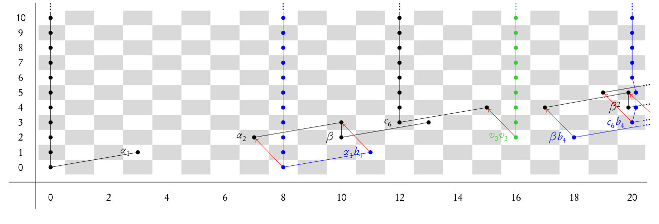 Figure 1
 Figure 2
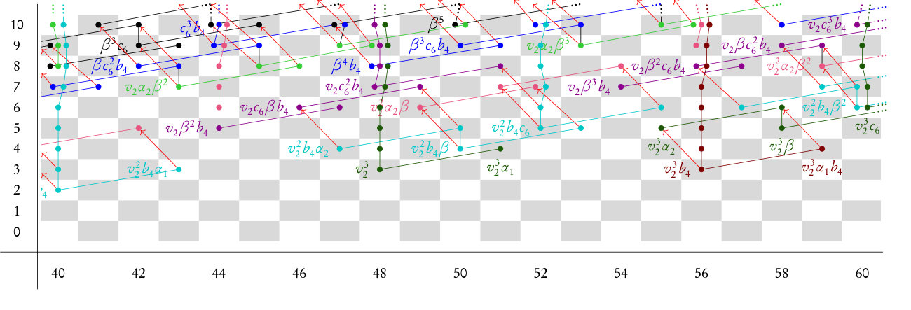 Figure 3
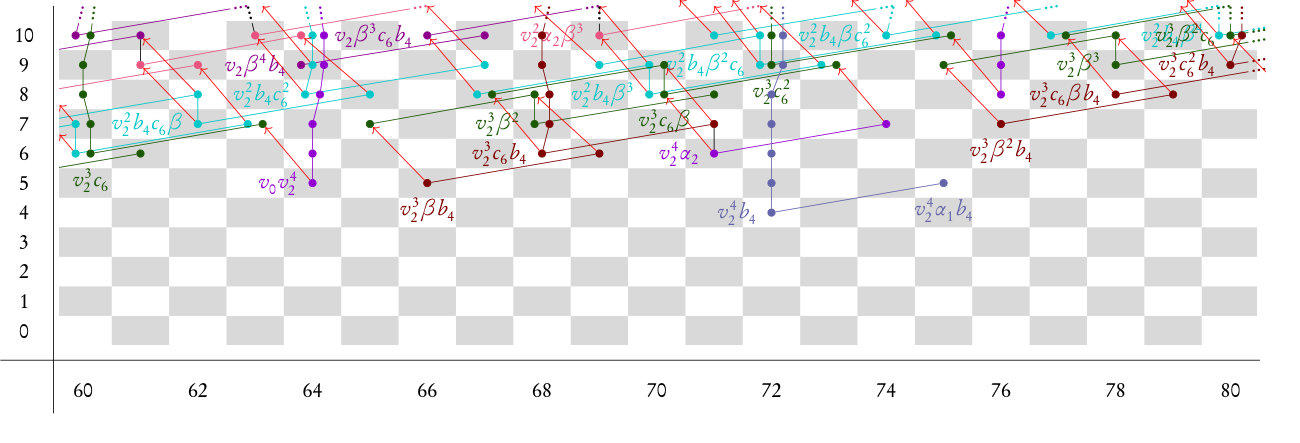 Figure 4
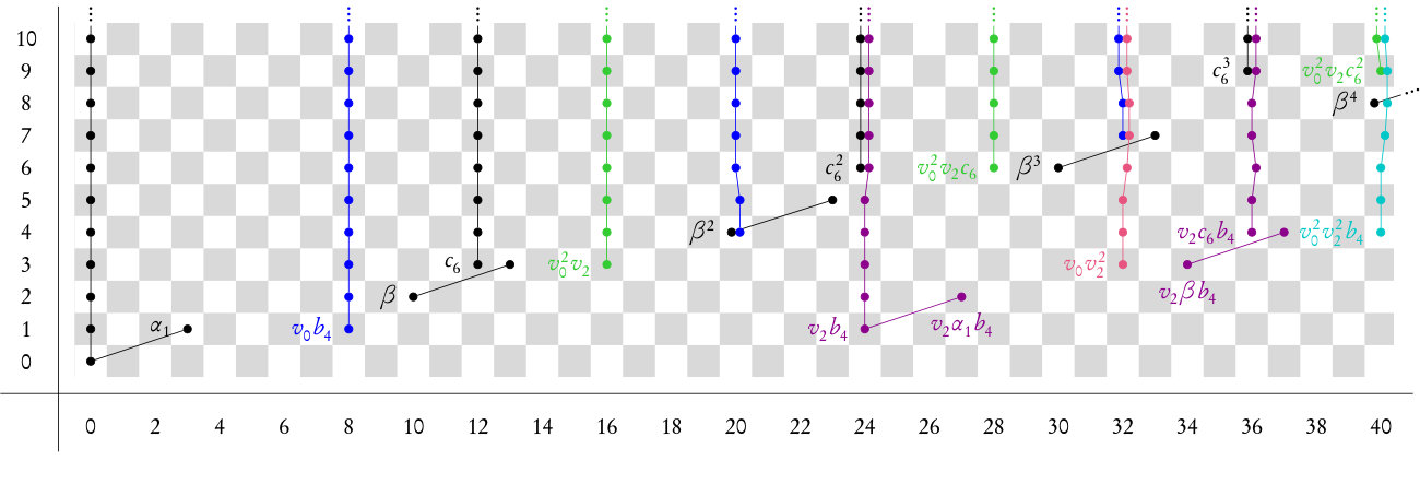 Figure 5
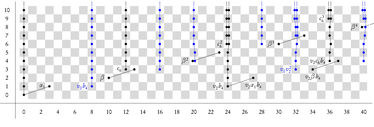 Figure 6
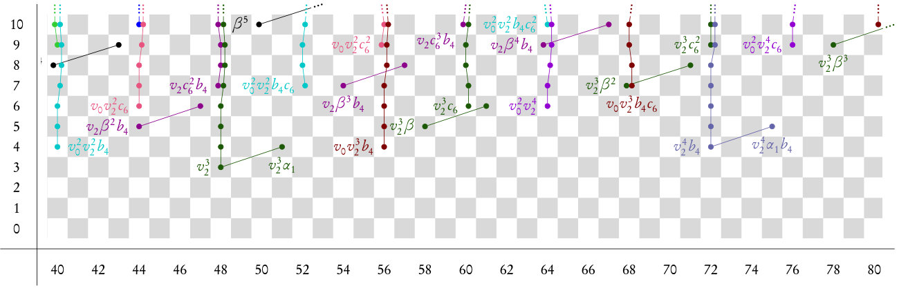 Figure 7
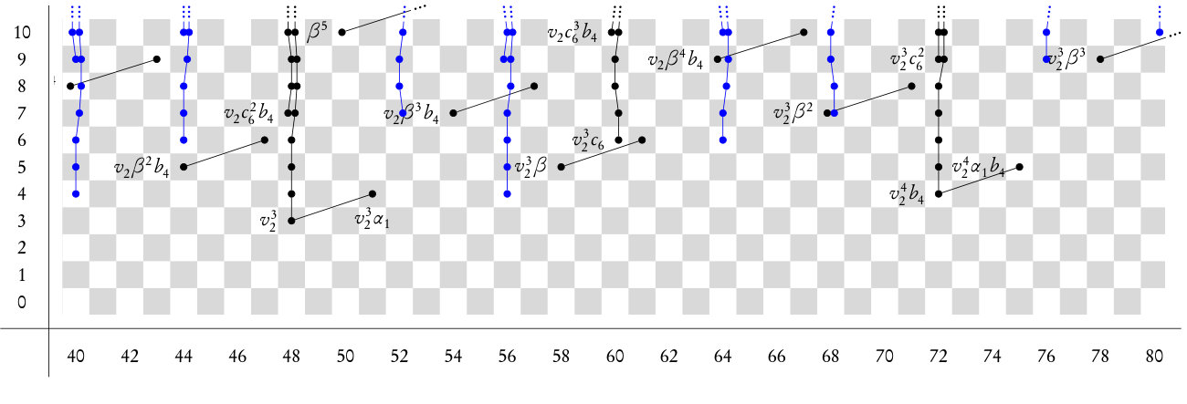 Figure 8
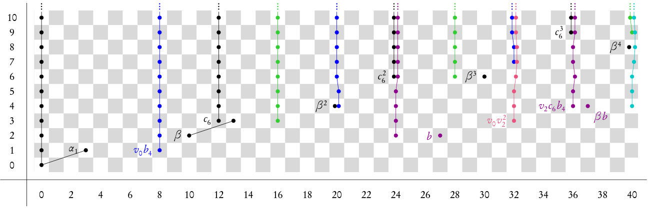 Figure 9
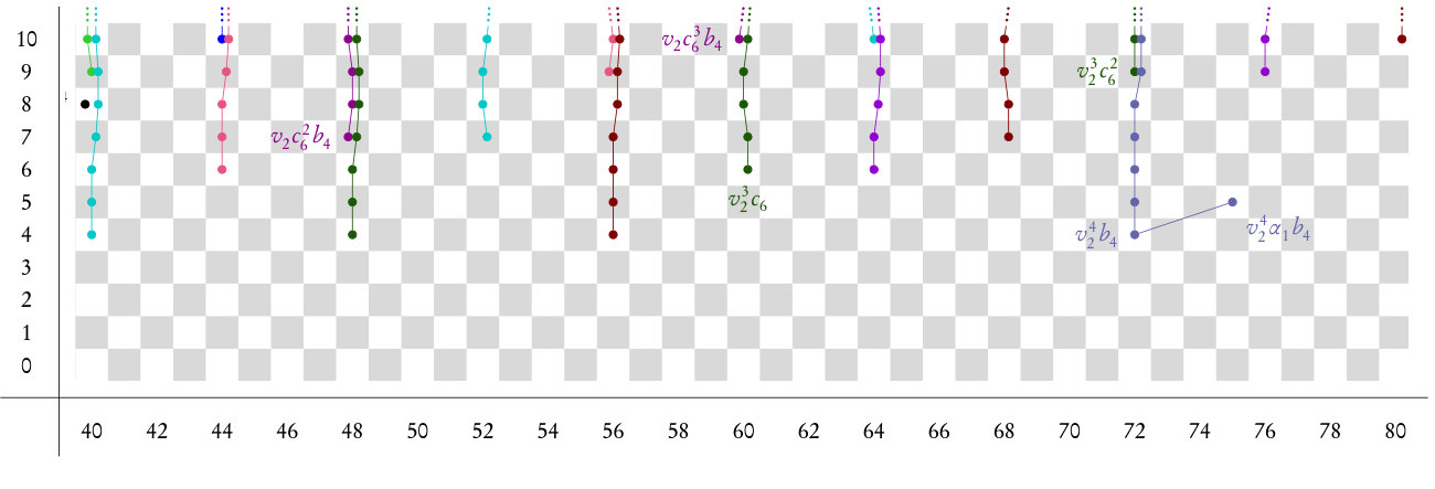 Figure 10
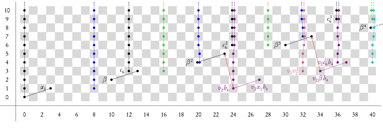 Figure 11
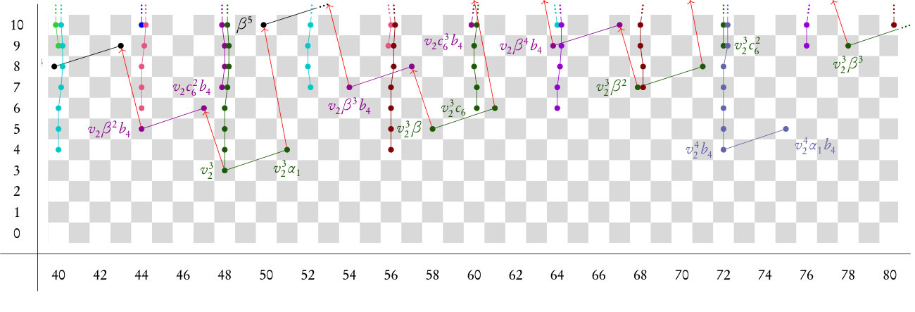 Figure 12
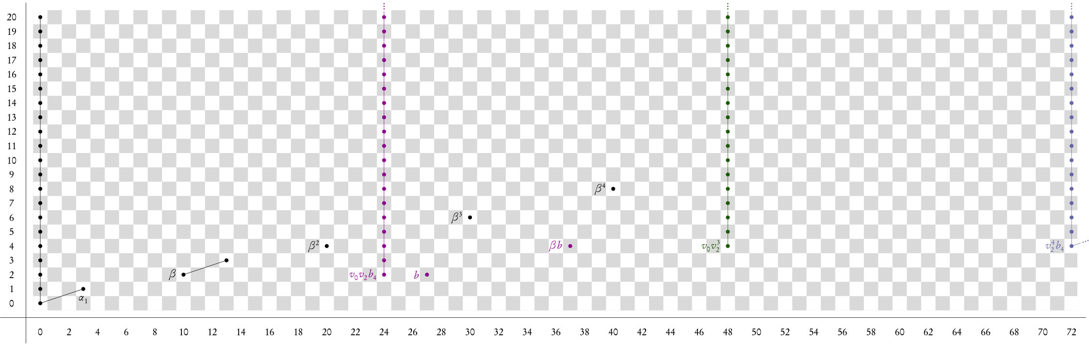 Figure 13
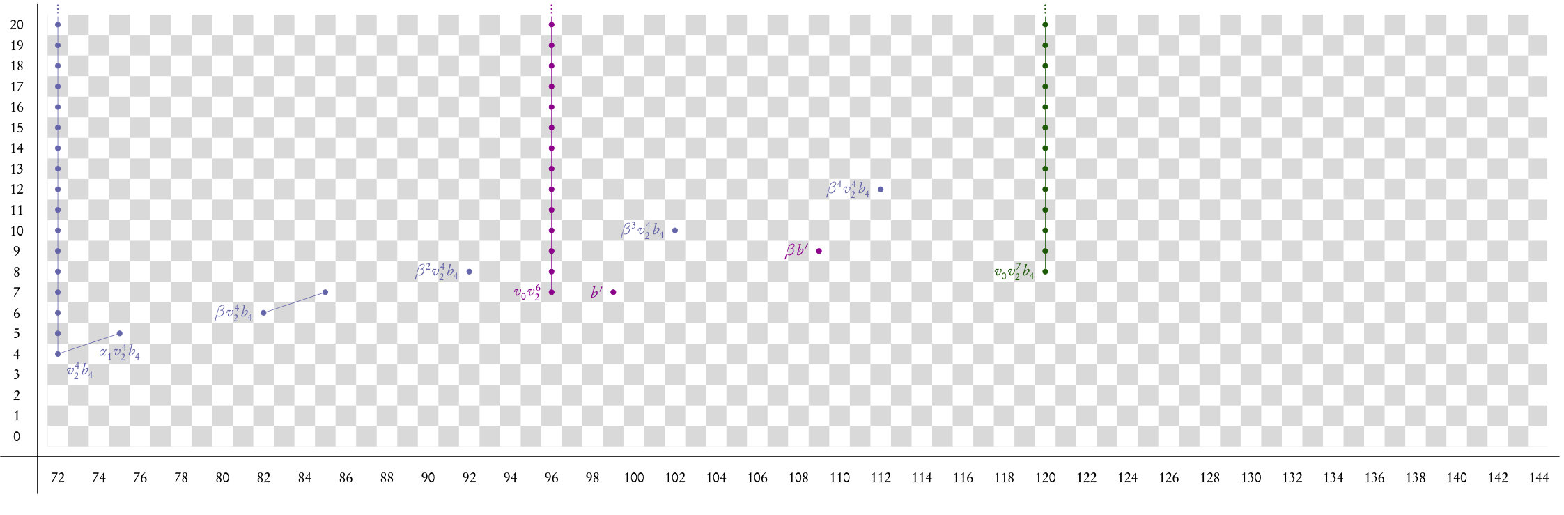 Figure 14
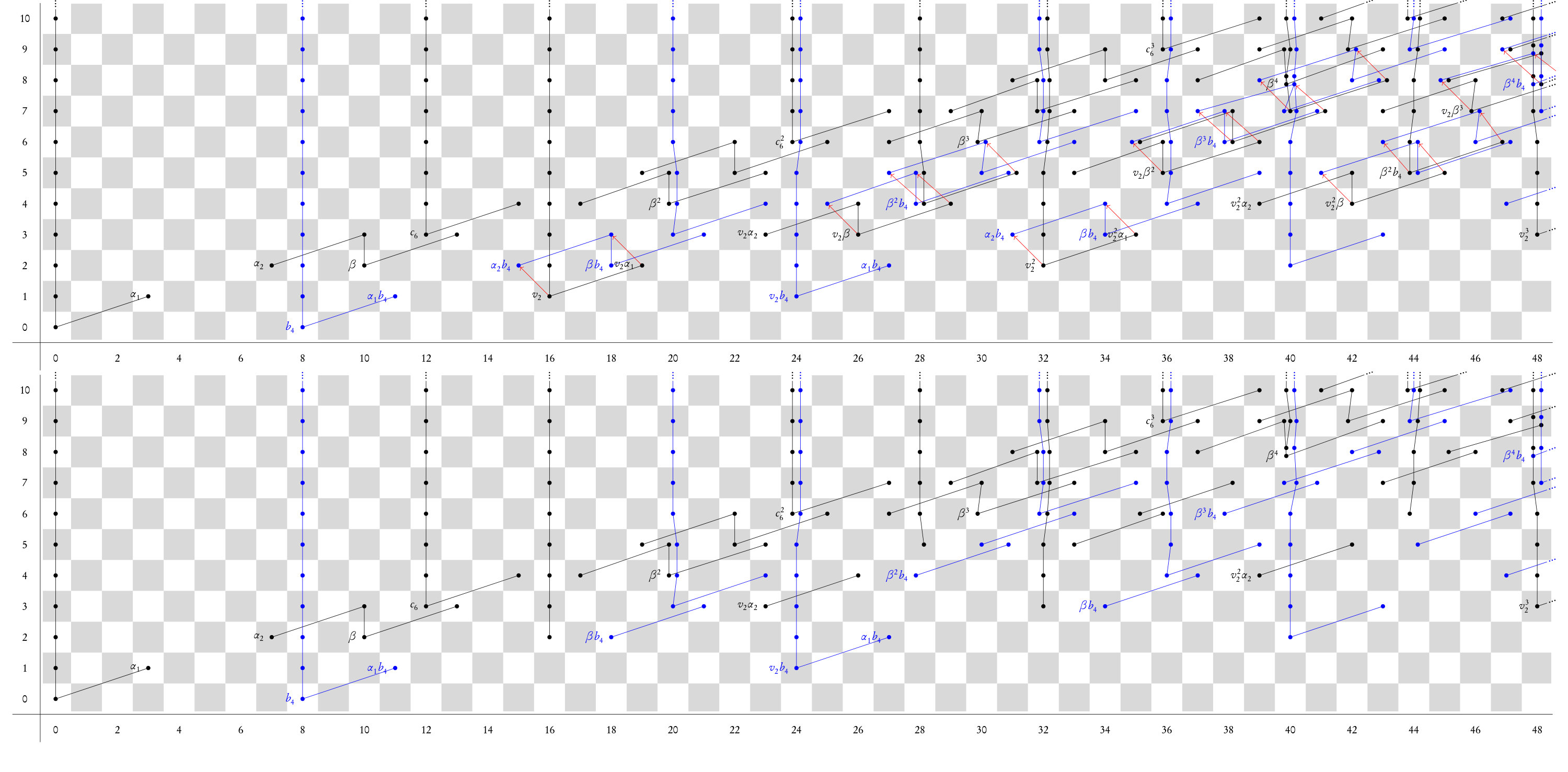 Figure 15
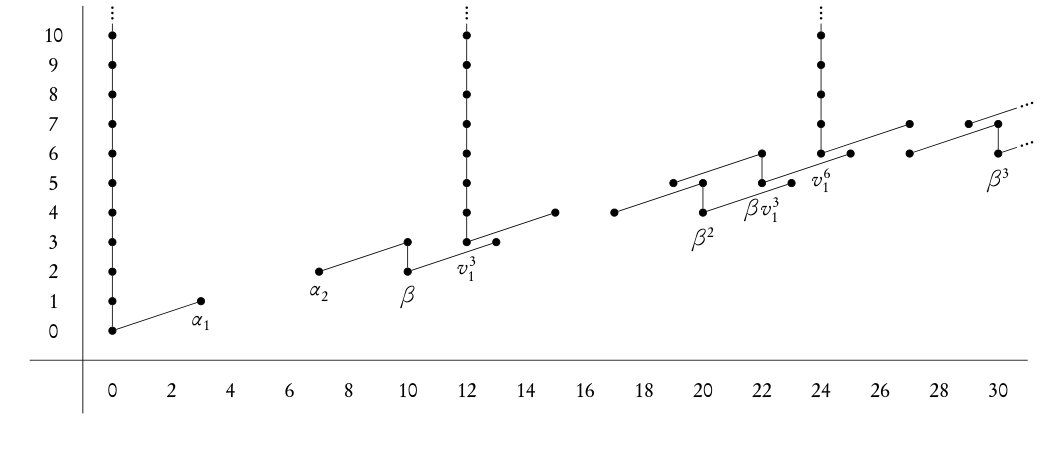 Figure 16
 Figure 17
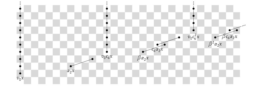 Figure 18
Peer Reviews
No public reviews on file for this paper yet. If you reviewed it on a platform where reviews are public (OpenReview, ICLR, NeurIPS, ICML), you can paste yours below so the community can read it here.
Videos
No videos yet. Explain this paper in a talk, walkthrough, or lecture? Add one.
The Adams spectral sequence for 3-local
D. Culver
University of Illinois, Urbana-Champaign
Abstract.
The purpose of this article is to record the computation of the homotopy groups of 3-local via the Adams spectral sequence.
Contents
1. Introduction
In this paper, we will carry out a computation of the homotopy groups of . The homotopy groups of have been known for quite some time. For example, the computation of was explicitly written up in [Bauer_2008], though it was known even earlier to Hopkins and Mahowald (cf. [MahowaldHopkins]). The usual approach to calculating the homotopy of and its variants is via the Adams-Novikov spectral sequence (also referred to as the descent spectral sequence in this context). One advantage of this approach is that the Adams-Novikov -term can be computed using the theory of elliptic curves.
However, there are occasions where one wants to know the Adams spectral sequence for computing the homotopy groups of a spectrum. That is, one may want to know the Adams -term, all differentials, and all hidden extensions. The purpose of this paper is to record the Adams spectral sequence for 3-local topological modular forms.
We should mention that the analogous calculation at the prime 2 is being carried out by Rognes and Bruner ([BrunerRognes]). It is the author’s understanding that their interest in that spectral sequence stemmed from their work on the topological Hochschild homology of . We speculate knowing the Adams spectral sequence at the prime 3 might be useful for similar reasons.
Conventions
In this article, we will implicitly assume that all spectra are 3-complete. Thus refers, from here on out, to the 3-completion of the spectrum of topological modular forms. We will always denote the mod 3 Eilenberg-MacLane spectrum by . Given a Hopf algebra and a comodule over , we will abbreviate by . In the case when , we will write . If for a spectrum , then we will abbreviate further to . We will always employ Adams indexing unless specifically stated otherwise. We let denote and denote in the dual Steenrod algebra. We will use the symbol to indicate equality up to a multiplicative unit. Finally, for a spectrum , we let denote the th page of the mod 3 Adams spectral sequence for .
1.1. Outline of the paper
Recall that the Adams spectral sequence is a convergent spectral sequence of the form
[TABLE]
Thus, a necessary input is . This was determined, for example, in [supplementary], where Rezk shows there is a short exact sequence of comodules
[TABLE]
where is a certain subalgebra of the dual Steenrod algebra . This is the starting point of our calculation. We view this short exact sequence as giving a multiplicative filtration of by comodules, yielding an algebraic spectral sequence
[TABLE]
In §2 we recall these details and establish a change-of-rings formula for . In §3 we use a Cartan-Eilenberg spectral sequence to compute . An expert in these affairs can safely ignore this section. In §4, we determine the Adams -term. In section §5 we discuss the rational homotopy of and its relationship to modular forms. Finally, in §6, we establish the Adams differentials and derive .
Acknowledgements
The author would like to thank Mark Behrens for encouraging him to write up this computation, as well as Bob Bruner for helpful discussions. He would also like to thank Hood Chatham for creating such a wonderful LaTeXpackage for drawing spectral sequences as well as for assistance in drawing some of the charts in this paper. Finally, the author thanks an anonymous referee for carefully reading earlier drafts of this paper. They caught many typos and errors and suggested improvements to the exposition, resulting in a better paper.
2. The mod 3 homology of
In this section we recall necessary facts about the mod 3 homology of . In [supplementary], it is shown that, as an algebra, the homology of is given by
[TABLE]
where and
[TABLE]
where the generators have the degrees
[TABLE]
Here, the are conjugate to Milnor’s element , and likewise is the conjugate of Milnor’s [greenbook, Theorem 3.1.1]. One can easily check that is a comodule algebra over . Note also that for degree reasons, the class is an -comodule primitive. Indeed, if
[TABLE]
then the degrees of are less than that of . But is the lowest positive degree element of .
Furthermore, Rezk shows that there is nontrivial extension of comodules
[TABLE]
Applying to this short exact sequence of comodules yields a long exact sequence in Ext. We regard this as a convergent spectral sequence
[TABLE]
The fact that 2.1 is a nontrivial extension implies that this spectral sequence does not immediately collapse. Determining the differentials in this spectral sequence is the subject of section 4. Thus, it is apparent that we need to compute the Ext groups of . We will simplify this by establishing a change-of-rings formula.
Definition 2.2**.**
Let be the Hopf algebra
[TABLE]
with the induced coproduct from the dual Steenrod algebra.
Example 2.3**.**
In the dual Steenrod algebra, the coproduct on is given by
[TABLE]
Thus, in , is a Hopf algebra primitive. On the other hand,
[TABLE]
Thus this Hopf algebra is not primitively generated.
The proof of the following proposition is standard.
Proposition 2.4**.**
There is an isomorphism
[TABLE]
We derive the following corollary from Theorem A1.3.12 of [greenbook].
Corollary 2.5**.**
There is a change-of-rings isomorphism
[TABLE]
Thus we must compute the cohomology of the Hopf algebra . This is done in the next section.
3. Computing the cohomology of
In the last section we showed that the Ext groups of are . Since is a finite Hopf algebra, there is hope of computing its cohomology. Recall that is the subalgebra of the Steenrod algebra generated by the Bockstein and . Its dual is
[TABLE]
In paticular, is a sub-Hopf algebra of . The following proposition relies on the material in the first appendix of [greenbook]. We recommend the reader look at Definition A1.1.15. The following lemma is easily checked.
Lemma 3.1**.**
The following
[TABLE]
is a cocentral extension of Hopf algebras over .
When one has an extension of Hopf algebras, one can consider the Cartan-Eilenberg spectral sequence. In general, if
[TABLE]
is an extension of Hopf algebroids, is a left comodule over , then there is a natural convergent spectral sequence of the form
[TABLE]
Here, denotes the filtration degree, is the cohomological degree, and is the internal degree. The differentials are of the form
[TABLE]
See A1.3.14 and A1.3.15 of [greenbook] for details on this spectral sequence. Applied to our extension of Hopf algebras with , this spectral sequence takes on the form
[TABLE]
Since is a primitively generated exterior Hopf algebra, we have that
[TABLE]
where the -bidegree of is . Note that since is a comodule algebra, the Cartan-Eilenberg spectral sequence is multiplicative.
In order to determine the -page of this spectral sequence, we need to understand the coaction of on . As is a comodule algebra over , it is enough to determine the coaction on .
Lemma 3.3**.**
Under the canonical -coaction on , the element is a comodule primitive.
Proof.
Observe that the largest degree element of is , which has degree 14. Since
[TABLE]
the coaction on must be for degree reasons. ∎
Corollary 3.4**.**
The -term of the Cartan-Eilenberg spectral sequence (CESS) is given by
[TABLE]
where is in -degree and is in tridegree .
Thus we must determine the cohomology of . The May spectral sequence can be used for this purpose. Later, we will need to use May’s convergence theorem to give a proof for Lemma 4.7, so we collect some details about the spectral sequence here. The reader is referred to [greenbook, 3.2] for further details.
This spectral sequence is obtained by putting a filtration on
[TABLE]
This filtration is defined by assigning the generators of the following May weight.
- •
,
- •
.
The associated graded of this filtration is given by
[TABLE]
but now with as primitive elements. This produces a filtration on the cobar complex for , resulting in the May spectral sequence
[TABLE]
with the following -term,
[TABLE]
Here we are using the fact that
[TABLE]
since are primitive and that
[TABLE]
since is primitive. The tri-degrees of these classes in the May spectral sequence are recorded below:
- (1)
, 2. (2)
, 3. (3)
, 4. (4)
.
Moreover, the -groups of primitively generated truncated polynomial algebras also have the following Massey product
[TABLE]
see [greenbook, Lemma 3.2.4]. Indeed, can be represented in the cobar complex for by
[TABLE]
which is precisely the Massey product above. Finally, the coproduct on gives the -differential
[TABLE]
The rest of the -differentials are propagated from this one and the multiplicativity of the May spectral sequence.
Proposition 3.5**.**
The algebra is given by
[TABLE]
where the -bidegrees of the generators are given by
- •
,
- •
,
- •
,
- •
,
- •
**
A chart for this Ext group is given below.
From now on, we will write for . This is justified by Proposition 5.5 below. For degree reasons, this spectral sequence collapses. Indeed, if we use -indexing to depict the Cartan Eilenberg spectral sequence -term, then a -differential goes up vertically -spaces. Since in degree , it follows there cannot be any differentials on .
Corollary 3.6**.**
The cohomology of the Hopf algebra is given by
[TABLE]
Proof.
We have already shown that this is the -page. All that remains to be shown is that there are no hidden extensions. First, note that in (3.2), denotes the filtration degree. Thus is in filtration 0. The Cartan-Eilenberg spectral sequence arises from an increasing filtration on a cochain complex (see [greenbook, A1.3.14, A1.3.16] for details). Thus, if and are two classes, then a hidden extension from to implies that the filtration of is larger than that of . Note also that there are no hidden extensions in the -submodule generated by 1. This is seen, for example, by noticing that the map induces a map in ,
[TABLE]
So, the only possible hidden extensions would involve products of classes in the ideal generated by . Suppose and are classes with . Then if , there could be a hidden extension to a class in higher filtration, let’s say there was an extension with . Note that in the usual Adams indexing the bidegrees must agree. Let us name the tri-degrees of these classes,
- •
- •
- •
.
Then the tri-degree of is
[TABLE]
whereas the tri-degree for is
[TABLE]
These classes detect elements in of bidegrees
[TABLE]
and
[TABLE]
respectively. These bidegrees must be equal, but in order for this to be a hidden extension, we must have . This implies that . Since is not a zero divisor on , it follows that it is not a zero divisor in . Thus, if we had the equality
[TABLE]
in , then we would have
[TABLE]
in . However, on , the only way we could have had is if . Since , it follows that in . This implies that . So there are no hidden extensions. ∎
4. Determining the Adams -term
In this section we will determine the -term of the Adams spectral sequence converging to . The way this will be achieved is by applying the functor to the short exact sequence (2.1) to obtain a long exact sequence. Regarding this as a spectral sequence provides us with
[TABLE]
For the purposes of this paper, we will refer to this spectral sequence as the algebraic spectral sequence.
4.1. Algebraic differentials
The short exact sequence (2.1) gives a multiplicative filtration of by -comodules. More precisely, we filter by setting and , the ideal generated by . Since is a comodule primitive, this is a filtration by comodules. The algebraic spectral sequence is then the spectral sequence associated to this filtration. Since the filtration is multiplicative, the spectral sequence is as well. Moreover, there is an isomorphism of -comodule algebras
[TABLE]
with concentrated in filtration degree 0 and a comodule primitive in filtration degree 1. Thus
[TABLE]
as a graded ring. Note that the bidegree of is . Since this spectral sequence arises from a long exact sequence in , there is only a -differential which has the form
[TABLE]
In depicting charts we will always use the Adams indexing convention and use the axes and suppress the filtration degree.
Below is a chart (Figure 4.1) for the -page of the algebraic spectral sequence. The classes in blue are those in the coset for in the -page. In other words, they have filtration 1 with respect to the filtration on . Note that the tri-degree of the -differential implies that all differentials originate from a black class and target a blue class.
We will now determine the differentials in the algebraic spectral sequence. First, we make the following simple observation.
Lemma 4.1**.**
For degree reasons, the classes , and are permanent cycles of the algebraic spectral sequence.
This observation and the multiplicativity of the spectral sequence eliminate many possible differentials.
From the known computation of (cf. [Bauer_2008]), we see that . In the -term of the algebraic spectral sequence, there are two classes in stem 15; the class and the class . Both of these classes must die, but for degree reasons the only possibility is the following differential111The class will be dealt with by an Adams differential.
[TABLE]
Multiplicativity of the spectral sequence and the previous lemma yields the following result.
Proposition 4.2**.**
The algebraic spectral sequence has the following -differentials
[TABLE]
for natural numbers and . There are no other differentials.
Consequently, this spectral sequence is periodic on the element .
Remark 4.3**.**
It would be nice to have an argument for this differential from first principles, but the author is not currently aware of one. He suspects this implies the existence of an interesting coproduct on .
4.2. Algebraic -term
We will now describe a few patterns which make up the -page of the algebraic spectral sequence. We will describe these patterns as certain modules over along with the monomial of the algebraic spectral sequence which generates it.
- (Pattern 1)
Since is a permanent cycle, we have the free modules on the powers of and the -multiples of , i.e. for all ,
[TABLE] 2. (Pattern 2)
For , we have the patterns
[TABLE] 3. (Pattern 3)
For , we have the following patterns
[TABLE]
The way we obtained these patterns was by noting that, as a module over , the -page of the algebraic spectral sequence is freely generated by the monomials . In other words, we have an isomorphism of -modules,
[TABLE]
The three patterns arise by partitioning the free modules into those which neither receive nor support any differentials (Pattern 1), receive differentials (Pattern 2), or support differentials (Pattern 3).
Remark 4.4**.**
In later parts of this paper we will need to refer to these patterns. We will refer to them as patterns of type on generator . So for example, if we look at the pattern on the Adams -term generated by the monomial , then we will call this a pattern of type 2 on generator . For patterns of the third type, we will call these patterns of type 3 on generator . This is potentially confusing since does not survive the algebraic spectral sequence unless is a multiple of 3. This terminology stems from the fact that this pattern is the residual piece of a free -module generated by .
4.3. Algebraic hidden extensions
As with any spectral sequence, there is the possibility of extension problems. We will show that there is a crucial hidden -extension which will play an important role in the next section. Namely,
Proposition 4.5**.**
In the algebraic spectral sequence, there is a hidden multiplicative extension
[TABLE]
consequently for every natural number and , we have the hidden extension
[TABLE]
Remark 4.6**.**
One might protest that this is not a hidden extension since is an element in the correct Adams filtration. However, from the perspective of the algebraic spectral sequence, has filtration 0 and has filtration 1. Since has filtration 0, this is in fact a hidden extension.
Before proving this, we will need to show the following.
Lemma 4.7**.**
In , there is the Massey product
[TABLE]
and there is zero indeterminacy.
To prove this, we need to recall May’s Convergence theorem. The proof of this fact can be found as Theorem 4.1 of [MR0238929], but we will only be interested in the case of a three-fold Massey product. The variant we will use is Theorem 2.2.2 of [StableStems]. However, since we are working at an odd prime, we have to keep track of signs. In the following, if is a class in degree , then we write for (see [greenbook, Appendix 4] for further details).
Theorem 4.8** (May’s Convergence Theorem).**
Let be elements of such that the Massey product is defined. For each , let be a permanent cycle on the May -page which detects . Suppose further that
- (1)
The Massey product is defined on the -page: there are and such that and . 2. (2)
If is the tri-degree of either or , and for for any and such that , the differential
[TABLE]
is zero.
Then the element is a permanent cycle and detects an element of .
Remark 4.9**.**
The second condition in May’s Convergence Theorem is often expressed by saying there are no “crossing differentials”.
We will use May’s convergence theorem to give a proof for Lemma 4.7. From the discussion of the May spectral sequence right before Proposition 3.5, is a non-zero permanent cycle. One easily shows that
Lemma 4.10**.**
In , there is the Massey product
[TABLE]
Proof of Lemma 4.7.
Since is exterior on the May -page, we get the following defining system and for the Massey product . This shows that on the May -page we have is in .
Since and in , the Massey product is defined in . Furthermore, there is no indeterminacy of this Massey product. So we just need to check the second condition of May’s Convergence Theorem, that there are no crossing differentials. Note that and that for all . So condition (2) is satisfied here. Likewise, note that and that for all . Thus there are no nonzero differentials to worry about. So condition (2) is always satisfied here as well. Thus we may apply May’s Convergence Theorem to infer that
[TABLE]
It is easy to see that there is no indeterminacy. ∎
Remark 4.11**.**
Keep in mind that May’s convergence theorem is actually very general (cf. the discussion preceeding [greenbook, A1.4.10]). It applies to any spectral sequence which arises from a multiplicative filtration on a DGA. In particular, it applies to the Cartan-Eilenberg SS and the algebraic SS we have used. Since the Cartan-Eilenberg SS collapses, and since the algebraic SS only has -differentials, the May Convergence Theorem vacuously applies to these spectral sequences.
Thus, we derive the following corollary.
Corollary 4.12**.**
In there is the Massey
[TABLE]
We will use this corollary to derive the hidden multiplicative extension.
Proof of Proposition 4.5.
One can check, using the May Convergence Theorem applied to the algebraic spectral sequence, that one has the Massey product
[TABLE]
and that this Massey product has no indeterminacy. Note that we do not know the sign since we only know the differential up to sign.
In order to apply the May Convergence Theorem to this Massey product, we must check that it is defined on . Note that in this Ext group, since there is no nonzero group in the 14 stem. Furthermore, since hidden extensions must always target a class in higher filtration, and since the algebraic spectral sequence only has elements in filtration 0 and 1, it follows that there can be no hidden extension for the product of and . Thus the Massey product is defined in (cf. Remark 4.11). Using the First Juggling Theorem (cf. [greenbook, A1.4.6]), we have
[TABLE]
yielding the desired extension. ∎
We will also have occasion to use the following hidden extension.
Corollary 4.13**.**
In the algebraic SS, there is the Massey product
[TABLE]
and consequently the hidden extension
[TABLE]
Proof.
A defining system for the Massey product on the page is given by and . Observe that there is no indeterminacy. So by May’s convergence theorem we have the Massey product
[TABLE]
Since this Massey product and are both strictly defined, we get from the First Juggling Theorem [greenbook, A1.4.6(c)] the following equalities
[TABLE]
∎
4.4. Comparison to the Adams spectral sequence in -modules
We now make a few remarks comparing the -term of the Adams spectral sequence for and the Adams spectral sequence for in -modules as studied by Hill ([Hill_2007, Section 2]). The latter is a spectral sequence
[TABLE]
where
[TABLE]
where is in degree 9. This class has an interesting coproduct, but this does not concern us here. What is interesting for us, however, is that in order to compute this coproduct, Hill filters ([Hill_2007, Theorem 2.2]), resulting in an algebraic spectral sequence
[TABLE]
One easily derives that
[TABLE]
where is the class represented in the cobar complex of by . In particular, . The term is concentrated in filtration degree 0. It turns out that this -page is in bijection with the -term of our algebraic spectral sequence, but with various elements in ours in the “wrong” filtration. For example, our element corresponds to Hill’s element . The former is in tridegree but the latter is in tridegree .
We provide a short dictionary relating various names in our spectral sequence to Hill’s algebraic spectral sequence.
[TABLE]
In particular, the element that Hill calls corresponds to the element we call . Moreover, Hill is able to derive a differential . Algebraic manipulation then yields the following differentials and . These all correspond to various differentials we encounter in this paper as well, but interestingly, not all of them are algebraic differentials. On the one hand, the differential corresponds to our algebraic differential . But the differential corresponds to an Adams -differential .
In particular, half of Hill’s algebraic differentials are seen in our algebraic spectral sequence, but the other half arise as Adams differentials. It is this discrepancy that makes the -relative Adams spectral sequence more computable as opposed to the absolute Adams spectral sequence.
5. Rational Homotopy of and modular forms
In this section, we examine the -inverted Adams spectral sequence for . In this case, the -inverted Adams spectral sequence converges to the rational homotopy groups of ,
[TABLE]
To determine the -localized Adams -term, we could take the decomposition from §4.2 and invert . Alternatively, we could use the -localized algebraic spectral sequence,
[TABLE]
The latter approach is more convenient. Note that
[TABLE]
This shows that the -localized algebraic -term is concentrated in even stems, and hence collapses at . Thus we find that
[TABLE]
and it follows immediately that the -localized ASS for collapses at .
The spectrum has a close connection to classical modular forms. The ring of integral modular forms, , has been known for quite some time.
Theorem 5.1** (cf. [CourbesElliptiqueFormulaire]).**
The ring of integral modular forms is given by
[TABLE]
Here, and are the normalized Eisenstein series of weight 4 and 6 respectively. Topologically, these have degree 8 and 12 respectively. The modular form is often referred to as the modular discriminant, and is a modular form of weight 12. The precise relationship between and integral modular forms is made by examining the Adams-Novikov spectral sequence. We need to make use of the following.
Theorem 5.2** (cf. [Bauer_2008], [Henriques]).**
The edge homomorphism for the Adams-Novikov spectral sequence for is a map
[TABLE]
where is the ring of classical integral modular forms. The image of this map contains and . Moreover, this map is a rational isomorphism.
Remark 5.3**.**
Since the edge homomorphism is a map of rings, the theorem determines the image entirely.
Corollary 5.4**.**
The rational homotopy groups of are given by
[TABLE]
Theorem 5.2 will allows us to determine what some of the elements in the Adams -term detect in . It will also be used to later to establish hidden multiplicative extensions in §6.4. We can carry some of this out even now.
Proposition 5.5**.**
The class in the Adams -term for survives to a non-zero element in and detects the class .
Proof.
It follows for degree reasons that cannot support or be targeted by a differential. This implies that survives to a nonzero element in . From Theorem 5.2, we know that some torsion free element in the 12 stem must detect . From the Adams spectral sequence calculation we see that the only -tower in stem 12 is the one generated by . Thus detects . ∎
6. Adams differentials
In this section, we will determine the differentials in the Adams spectral sequence for . Since is a commutative ring spectrum, the Adams spectral sequence is multiplicative. Begin by noting that there are several classes which are permanent cycles for degree reasons.
Lemma 6.1**.**
The classes , and are all permanent cycles for the Adams spectral sequence. Consequently, the differentials in the Adams spectral sequence are linear over .
This observation is very useful for our calculation for the following reason. In the last section, we have expressed the Adams -term as a direct sum of certain patterns which were modules over . This observation implies that the only nonzero -differentials in the Adams spectral sequence will originate on the monomials which generate these patterns. We will also make frequent use of the following facts about .
Theorem 6.2** (cf. [Henriques]).**
The homotopy groups of are 72 periodic. Furthermore, the torsion in is concentrated in stems 3, 10, 13, 20, 27, 30, 37, and 40 modulo 72.
We will begin by determining all of the length 2 differentials.
6.1. Adams -differentials
As was mentioned previously, the Adams differentials are all linear over , which means we only have to figure which of the following families of monomials support Adams -differentials: For any natural number
- (1)
, 2. (2)
, 3. (3)
for , and 4. (4)
for .
From our charts (Figures 6.1 and 6.2 below), one sees that can support a length 3 differential at minimum. Thus, is a -cycle for all . Moreover, there are several multiplicative relations on the Adams -term which we get from the previous section. For example, we have . Consequently, we have
Proposition 6.3**.**
The Adams -differentials for are linear over . Thus, we only need to determine which of the monomials , , , , , , and support -differentials.
Proposition 6.4**.**
There is an Adams -differential
[TABLE]
Proof 1.
From the known computation of , it is seen that . Thus, the class must die. The only possibility is the claimed differential. ∎
Proof 2.
Recall that in the Adams -term for , we have the Massey product
[TABLE]
In the homotopy groups for the sphere, there is the same Toda bracket by Moss’ convergence theorem (see [Moss_1970] or [StableStems, Theorem 3.1.1]). Note also that is represented in the cobar complex by .
In the Adams -term for , there are classes of the same name and the same Massey product holds. In the cobar complex for , the class is also represented by . Thus, under the induced map on groups
[TABLE]
is sent to . The Massey product then shows that is mapped to . Hence, and are in the Hurewicz image of the sphere.
It is known from the Adams spectral sequence for the sphere that there is a -differential whose target is (cf. [greenbook, Figure 1.2.15]). Since is in the Hurewicz image, it follows that in . This forces the Adams differential
[TABLE]
However, as is a permanent cycle for the ASS for , we must have that
[TABLE]
as stated. ∎
Remark 6.6**.**
This is one of the Adams differentials which occurs as an algebraic differential in [Hill_2007].
We can draw an interesting consequence from the second argument provided above (we learned this from Mike Hill and Mark Behrens).
Corollary 6.7**.**
The element is the image of under the map
[TABLE]
and consequently we have the hidden comodule extension in ,
[TABLE]
where denotes the -coaction on .
Proof.
In the Adams spectral sequence for the sphere, it is the class which supports a -differential killing . Naturality of the Adams spectral sequence implies that maps to .
In the cobar complex for , the element is represented by . On the other hand, we can represent in the cobar complex for by . Thus there must be an element of which bounds the difference between and . The only possibility is
[TABLE]
This implies the claimed coaction. ∎
Proposition 6.8**.**
There is an Adams -differential
[TABLE]
Proof 1.
It is known that . The only nonzero class in this stem on the Adams -term for is . Thus, this class must die. The only possibility is the claimed differential. ∎
Proof 2.
We provide a second proof which does not rely on a priori knowledge of . Recall the Massey product for we found in Corollary 4.12. Since projects to 0 on the -page, we have that the Massey product projects to 0 at . One also checks that the indeterminacy for this Massey product on is 0. It is also the case that there is no room for crossing differentials in this range. Thus Moss’ Convergence Theorem ([Moss_1970], [StableStems, Theorem 3.1.1]) implies that must project to 0 in . This implies that must be killed by a -differential. The only possibility is the claimed differential. ∎
One might be tempted to conclude from this that there is a length 2 differential from to . However, one must be cautious. Even though was a product in the -term of the algebraic spectral sequence of the last section, it is no longer decomposable (as supported an algebraic differential). In fact, this differential does not occur. As explained in subsection 4.4, the classes and correspond to Hill’s classes and respectively. Also, corresponds to , the modular discriminant. In any of the computations for , there is a differential . This suggests that ought to support a length 3 differential to . On the other hand, , and on , there are the nonzero classes , and . Also, Proposition 6.4 implies that , taking care of the class . This suggests that will support a differential.
Proposition 6.10**.**
In , one has that . Consequently, there is an Adams -differential
[TABLE]
We give two proofs.
Proof 1.
By the previous proposition, we can form the Massey product on the -page. By the juggling lemma, [greenbook, Appendix 1], we have that
[TABLE]
From the previous proposition, we infer that the Massey product contains 0. It is also easy to see that this Massey product has zero indeterminacy. Thus in . Thus must be the target of a -differential. The only possible source is . ∎
Proof 2.
From Proposition 6.4, we deduce that
[TABLE]
The hidden extension 4.13 then implies the stated differential. ∎
The next monomials we need to consider are , and , in that order. By inspection of the chart, each of these classes have only one possible target on the -page. However, one finds from the previous propositions that each of these potential targets actually supports a differential. Thus , and are -cycles. Thus we move on to the monomial .
Proposition 6.12**.**
There is a -differential
[TABLE]
as well as the -differential
[TABLE]
Proof 1.
It is known that is zero (cf. [Bauer_2008, supplementary]), but on the -term, there are the nonzero classes and which are not killed by previously established -differentials. The only way for to be killed is by a -differential given by the claimed differential. The hidden -extension established in Proposition 4.5 gives us the second differential. ∎
Proof 2.
We have already established the differential . Since is a -cycle, we have that
[TABLE]
However, in the algebraic spectral sequence, we had the relation
[TABLE]
The multiplicativity of the spectral sequence and the hidden extension in Proposition 4.5 implies the differential . ∎
We can draw from this differential another -differential.
Corollary 6.15**.**
There is the following -differential
[TABLE]
Proof.
From the previous proposition we deduce the differential
[TABLE]
However, we have from Proposition 4.5 that
[TABLE]
This implies the differential
[TABLE]
However, since , we also have
[TABLE]
Since is a permanent cycle, multiplicativity of the spectral sequence implies the claimed differential. ∎
This completes the determination of the Adams -differential. Below, in Figure 6.1 and 6.2, we depict that Adams -term along with the -differentials. The reader will notice that we have used several different colors in the chart. Here is a key to the use of these colors.
[TABLE]
.
Before proceeding onto computing the -differentials, we will give a description of the Adams -term based on the differentials we just found.
6.2. Determining the Adams -term
We now set out to determine the patterns that make up the Adams -term for . To get things going, first note that the pattern of type 2 on generator and the pattern of type 3 on generator support differentials into the pattern (see Remark 4.4 for an explanation of this terminology). More specifically, the differential (6.5) propagates to give the following -differentials for and ;
[TABLE]
Similarly, the differentials (6.9) and (6.11) respectively propagate to give the differentials
[TABLE]
and
[TABLE]
Observe that any monomial in involving an or a is hit by a differential. So from we obtain the module
[TABLE]
The patterns supported by and do not receive any Adams -differentials, so all we must do is determine what remains of these patterns after applying the Adams -differentials. It follows from these differentials that what remains of the pattern on is the submodule
[TABLE]
and what remains of the pattern on is
[TABLE]
The next pattern we need to consider is the pattern of type 2 on . Since is a -cycle, this entire pattern consists of -cycles. Because of the hidden -extension in Prop 4.5, we will consider this pattern in tandem with the half of the pattern of type 3 on generated by ; namely the module . This half also consists only of -cycles. Thus, the combined pattern only receives differentials. It receives its differentials from the free pattern . The differentials (6.13), (6.14), and (6.16) propagate to give the following differentials:
[TABLE]
Note that any monomial in the pattern which contains a or is hit by a differential. Also, the piece is annihilated by these differentials. Hence, this pattern yields the following module
[TABLE]
It also follows that what remains of the pattern on is the submodule
[TABLE]
The other half of pattern 3 on , i.e. , consists entirely of -cycles and receives no differentials. Thus this survives in full to the -page.
As we have already mentioned, the Adams -term for is periodic on . Combining all of these observations proves the following identification of the Adams -term.
Proposition 6.17**.**
The Adams -term is given as a module over as the infinite direct sum of the following types of modules,
- Pattern 1’
For all , we have the modules
[TABLE] 2. Pattern 2’
For all , we have the modules
[TABLE]
and the ring structure is inherited from the Adams -term.
We give the Adams chart for the -term below in Figure 6.3. We have given two copies of this chart, one inheriting the colors from previous charts, the other where we depict Pattern 1’ in black and Pattern 2’ in blue.
As we will see later, will detect the class . Similarly, the class will detect . On the other hand, there are certain important classes in the Adams-Novikov spectral sequence which support differentials. Namely, the class . In the ANSS, . In the ASS, the class corresponds to while the class corresponds to . The class corresponds to the class , while the class corresponds to . The reader should note that, at the -page, we do not have that . In fact, is not in the correct filtration for this to happen. This what makes the Adams spectral sequence more difficult than the analogous calculation in [Hill_2007]. However, since is periodic on , this does suggest re-expressing the -term in the following way. Let denote the -module
[TABLE]
In other words, is the collection of all the patterns from Proposition 6.17 which are generated by the listed monomials in degrees less than . The following now follows from the previous proposition.
Corollary 6.19**.**
There is an isomorphism of -modules
[TABLE]
Remark 6.21**.**
We will see that the classes detect the elements , while the classes will detect the elements .
Remark 6.22**.**
It might be easier for the reader to regard as being comprised of three pieces. Let and define
[TABLE]
Then
[TABLE]
At this point the Adams -term is “isomorphic” to the Adams-Novikov -term but with the elements in the “wrong” filtrations. All of the later differentials correspond to the usual differentials in the Adams-Novikov spectral sequence, and in fact we could deduce them from that spectral sequence. However, we try to provide arguments from first principles below.
6.3. Higher Adams differentials
The Adams -term for is much sparser than the -term. This greatly reduces the possiblity of higher Adams differentials. We will now determine the , , and differentials in the Adams spectral sequence for . First, we make the following observation.
Proposition 6.23**.**
The elements in Pattern 2’ of Proposition 6.17 are permanent cycles. Furthermore, this pattern receives no -differentials.
Proof.
Since the higher Adams differentials are linear over , it suffices to check that the generators of Pattern 2’ are permanent cycles. These are the elements . Note that these are all in even degree, so their potential targets are in odd degree. From Proposition 6.17, the only elements of odd degree on the -term are of the form or .
Recall that , so the degrees of the generators for Pattern 2’ are congruent to [math] or mod 16. On the other hand, the degrees of the potential targets are congruent to or mod 16. This shows the generators of Pattern 2’ cannot support a differential for degree reasons. Similar considerations show that these elements cannot be the targets of any -differentials. ∎
Recall that the unit map
[TABLE]
for induces a map in Ext taking the class to and to . This is used in the calculation [Bauer_2008] to derive higher Adams-Novikov differentials. We will also use it to derive higher Adams differentials.
Proposition 6.24**.**
There is an Adams -differential
[TABLE]
Proof.
It is known that . The only non-zero class in that stem on the -term is . This forces the stated differential. ∎
Remark 6.25**.**
The author has made attempts to give an argument for this differential from first principles. But as of the writing of this article, he has been unable to find one.
Proposition 6.26**.**
There is an Adams -differential
[TABLE]
Proof.
Since the classes and are both in the Hurewicz image of , so are all the monomials . In the stable homotopy of , the class is zero (see [greenbook, Figure 1.2.15]). Since the corresponding class in is not zero, it must be hit by a differential. The only possible class which could support a differential to is . Thus we have the -differential
[TABLE]
As the Adams differentials are linear over , we infer
[TABLE]
∎
Remark 6.27**.**
Recall that corresponds to the class in the relative Adams spectral sequence (or in the Adams-Novikov spectral sequence). In particular, this differential corresponds to the -differential in [Hill_2007]. In that spectral sequence, this implies the differential . However, in the ASS, the class squares to 0, so we cannot establish such a -differential. Rather it corresponds to the -differential we established in Proposition 6.24. It is interesting to note these -differentials in the relative ASS get decoupled in the ASS.
Remark 6.28**.**
One might like to think that there is the -differential
[TABLE]
because one can multiply the differential on to get this differential. But this is not the case since supports a shorter differential. This is an important occurrence in this spectral sequence because is detecting the class and the homotopy groups of are famously periodic on .
For degree reasons, these are the only possible and differentials. We will now produce the last differential in the Adams spectral sequence. In order to do that, we will need the following observation.
Lemma 6.29**.**
The class is given on the -page as the following Massey product
[TABLE]
Thus, by Moss’ Convergence Theorem, the class in is given by the corresponding Toda bracket.
Proof.
The differential gives a defining system for the Massey product on the -page, and there is zero indeterminacy. Furthermore, the Toda bracket is defined. Since there are no differentials up to the 30 stem after the -page, there are no crossing differentials to worry about. So by Moss’ convergence theorem, is given by the associated Toda bracket. ∎
Proposition 6.30** (compare with [Bauer_2008, Goerss_2003]).**
There is the following hidden multiplicative extension in ,
[TABLE]
Proof.
Recall that is given by the Toda bracket . So, by the first juggling lemma (cf. [greenbook, Appendix 1]), it follows that
[TABLE]
∎
Corollary 6.31**.**
The class is 0 in the homotopy groups of . Thus, there is a -differential
[TABLE]
Proof.
Using the multiplicative extension of the previous proposition, we have
[TABLE]
Since , we have that in . This forces the claimed differential. ∎
Thus far, we have only produced higher Adams differentials on generators in the submodules and of (see Remark 6.22). There remains the summand . Multiplication by propagates the differential from Proposition 6.24 to a differential
[TABLE]
Unfortunately, as in Remark 6.28, we cannot multiply by to infer differentials on or . However, [Moss_1970, Theorem 1.1] tells us that we have a Leibniz type rule for differentials on Toda brackets. We will use this to derive the desired differentials.
Lemma 6.32**.**
The class is a permanent cycle.
Proof.
The only possible differential that could have supported was a -differential to . But we have already shown that this class supports a -differential in Corollary 6.31. ∎
Proposition 6.33**.**
There is the following Massey product on the -page of the Adams spectral sequence for ,
[TABLE]
Consequently, we have that
[TABLE]
Proof.
A defining system for the first Massey product arises from the differential . There is no indeterminacy, hence we have an equality. Since and are permanent cycles, the differential is an immediate consequence of [Moss_1970, Theorem 1.1]. ∎
We would like to derive a -differential on to . The argument will be similar to the one found in Corollary 6.31.
Proposition 6.34**.**
The class is given on the -page by the Massey product
[TABLE]
By Moss’ convergence theorem this class survives to a class in given by the corresponding Toda bracket. Consequently, there is the hidden extension
[TABLE]
in .
Proof.
The argument is completely analogous to the one in Lemma 6.29. Alternatively, we can derive this from Lemma 6.32 below by using a juggling theorem for Toda brackets
[TABLE]
Keep in mind these are Toda brackets in . We can do this since is a permanent cycle. The Toda bracket on the right hand side has indeterminacy in (see [Kochman:1996aa, Proposition 5.7.2(b)])
[TABLE]
It is seen on the -page that . Thus there is no indeterminacy. ∎
Proposition 6.35**.**
The class is 0 in . Thus there is the -differential
[TABLE]
Thus we have analogs of the differentials in Proposition 6.26 and Corollary 6.31 in the summand of .
Now we move on to showing is a permanent cycle.
Proposition 6.36**.**
The class is a permanent cycle.
Proof.
Note that is in stem 144. Thus, any higher Adams differential supported by must live in odd degree. The only odd degree elements in the -term live in Pattern 1’ in Proposition 6.17. In fact, since the generators of these patterns, or , are in even stems, it follows that the only possible targets of a differential on are of the form or . By examining the degrees of these elements, we see that the only ones in degree 143 are or .
The first option could be the target of a -differential, but it follows from Proposition 6.24, Lemma 6.32, and multiplicativity that supports a -differential targeting . If, however, where hit by a -differential with , then we would not be able to exclude as a target of a -differential. However, this cannot happen since the only elements in stem 143 on the -page are and .
The other option, could be the target of a -differential, but the target is hit by an earlier -differential supported by . Thus is a permanent cycle.
∎
We can now derive that the Adams spectral sequence for collapses at . Towards this end, let denote subquotient obtained from by incorporating the to -differentials. Then we have the decomposition
[TABLE]
Below, in Figure 6.5, is a depiction of . The reader should note the chart for in stems and in stems are identical up to a shift in Adams filtration. This is explained by the fact that will detect the class (Corollary 6.43), which is the famous periodicity generator.
Proposition 6.38**.**
The submodule consists of permanent cycles. Consequently, the Adams spectral sequence for collapses at .
Proof.
Since the Adams -term is periodic on , it is sufficient to check that there are no differentials supported by the indecomposable elements of . It is easily seen from Figures 6.5 that the elements originating from Pattern 1’ in the -term cannot support -differentials whose target is also an element originating from Pattern 1’. This leaves the possibility of the indecomposable classes supporting differentials into pattern 2’.
Since Pattern 2’ is concentrated in even degrees, this excludes the possibility of the indecomposable classes from supporting differentials; hence these classes are permanent cycles. The classes and may support differentials into Pattern 2’. Since the differentials are linear over , we are reduced considering the classes and .
Observe that generators of Pattern 2’ are all in stems congruent to 0 mod 8. On the other hand, and are in stems 27 and 99 respectively. Observe that these are congruent to 3 modulo 8. Thus, the degree of a possible target of a differential supported by or must lie in degree congruent to 2 mod 8. Since all of the elements of Pattern 2’ are in stems congruent to 0 modulo 8, and cannot support differentials into Pattern 2’. As we have already mentioned, and also cannot support differentials into Pattern 1’. Thus and are permanent cycles.
This shows that all of the elements of are permanent cycles. Since is a periodicity generator for , it follows from Proposition 6.36 and the fact that the ASS for is multiplicative that . ∎
We provide the Adams -term along with all higher differentials as well as a chart for the -term below in Figures 6.6 and 6.7
6.4. Hidden extensions
In the previous subsection we showed that the Adams spectral sequence for collapses at and we completely computed this page via (6.37). We’ve already established one hidden extension in Proposition 6.30, which corresponds to the single hidden extension occurring in the Adams-Novikov spectral sequence for .
However, there are several relations in which are apparent on the Adams-Novikov -page appearing in the 0-line, but which are hidden from the perspective of the Adams spectral sequence. We make several observations.
Proposition 6.39**.**
The class in detects the class in up to a unit.
Proof.
From Theorem 5.2, the modular form is in . Since is of degree 8 and a torsion free class, it must be detected by a class in stem 8 in the -page which supports an entire -tower. The only such class is . ∎
Looking at our chart for , we find that there is a single -tower in the -stem which is generated by . This implies the following,
Proposition 6.40**.**
The class detects the class in and we have the hidden extension in the -term.
Remark 6.41**.**
In light of Proposition 6.39 and Proposition 5.5, we will abuse notation and write as and as .
We can also say which classes are detecting the various classes involving in . We will rename some classes in order to give more streamlined expressions. We will rename by . Thus, for example, the class refers to . We will use the expression , when , to mean , while when this expression stands for . At the moment, we have introduced this notation more for convenience, it is not reflective of a multiplicative structure on any page of this spectral sequence. Indeed, on , the square of is 0. However, this notation is motivated by a certain hidden extension which will appear shortly.
Note that from the results of the previous section, we have
Lemma 6.42**.**
When , the classes support a differential, and in this case the classes are permanent cycles.
We can determine what these classes detect in .
Corollary 6.43**.**
For , the classes detect up to a unit. For , the class detects , up to a unit.
Because these correspond to multiples of powers of , this implies a family of hidden extensions.
Corollary 6.44**.**
In , we have the following hidden extensions for every ,
[TABLE]
We have the hidden extensions for odd
[TABLE]
This corollary justifies our choice of notation. Finally, Theorem 5.2 and the famous relation of modular forms
[TABLE]
implies a hidden extension in the -term.
Proposition 6.45**.**
There is a hidden extension in given by
[TABLE]
These hidden extensions, of course, propagate themselves throughout the -term. There are no hidden extensions beyond the ones mentioned above.
Remark 6.46**.**
It is rather unsatisfying that these hidden extensions were determined by using the known multiplicative structure in . It would be nice to have arguments from first principles. It would seem that this would require knowing Massey product descriptions of various classes, such as , and so on. But the author was unable to find such descriptions.
References