Emission of photon pairs by mechanical stimulation of the squeezed vacuum
Wei Qin, Vincenzo Macr\`i, Adam Miranowicz, Salvatore Savasta, and, Franco Nori

TL;DR
This paper proposes a feasible optomechanical method to observe the dynamical Casimir effect through mechanically-induced photon pair emission, avoiding the need for ultra-high mirror velocities or strong coupling.
Contribution
It introduces a novel approach using detuned parametric driving to amplify the dynamical Casimir effect in an optomechanical system without extreme physical requirements.
Findings
Demonstrates mechanically-induced two-photon hyper-Raman scattering.
Shows that small squeezing can significantly amplify the DCE.
Provides a practical implementation pathway for observing DCE.
Abstract
To observe the dynamical Casimir effect (DCE) induced by a moving mirror is a long-standing challenge because the mirror velocity needs to approach the speed of light. Here, we present an experimentally feasible method for observing this mechanical DCE in an optomechanical system. It employs a detuned, parametric driving to squeeze a cavity mode, so that the mechanical mode, with a typical resonance frequency, can parametrically and resonantly couple to the squeezed cavity mode, thus leading to a resonantly amplified DCE in the squeezed frame. The DCE process can be interpreted as {\it mechanically-induced two-photon hyper-Raman scattering} in the laboratory frame. Specifically, {\it a photon pair} of the parametric driving absorbs a single phonon and then is scattered into an anti-Stokes sideband. We also find that the squeezing, which additionally induces and amplifies the DCE, can be…
Click any figure to enlarge with its caption.
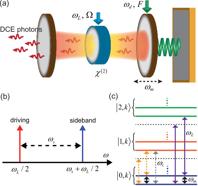 Figure 1
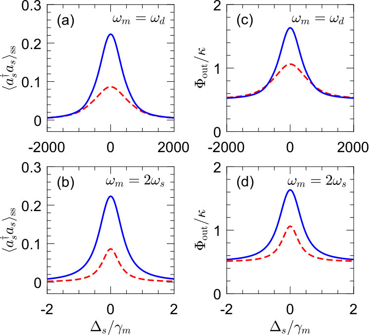 Figure 2
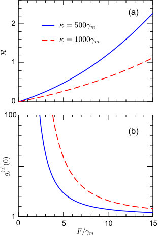 Figure 3
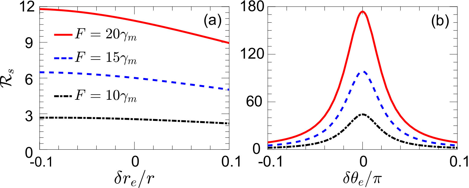 Figure 4
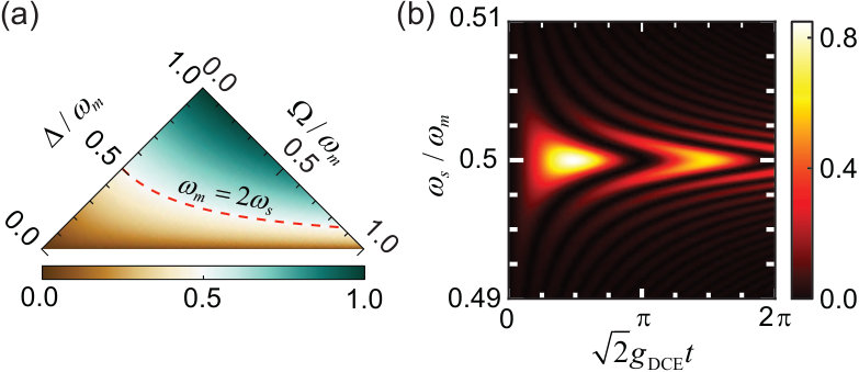 Figure 5
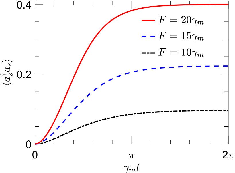 Figure 6
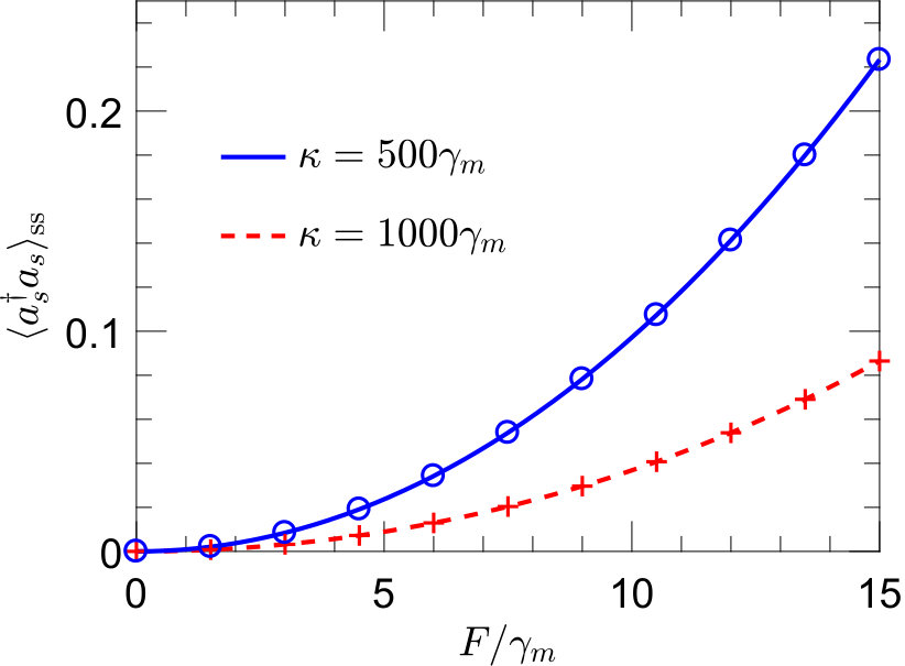 Figure 7
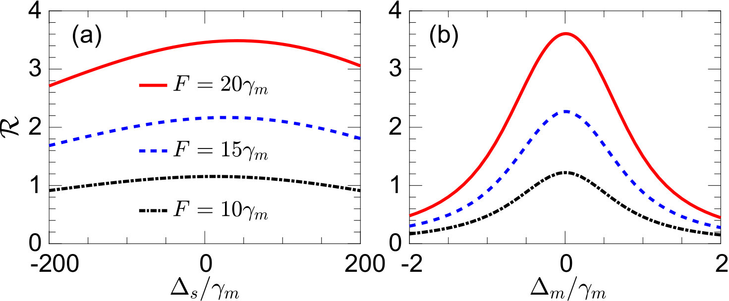 Figure 8
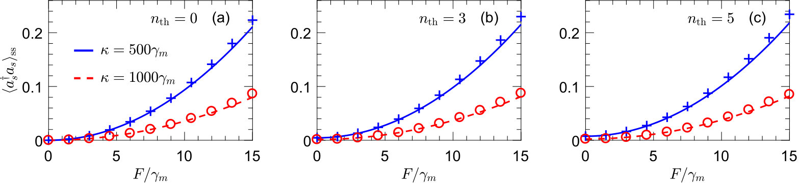 Figure 9
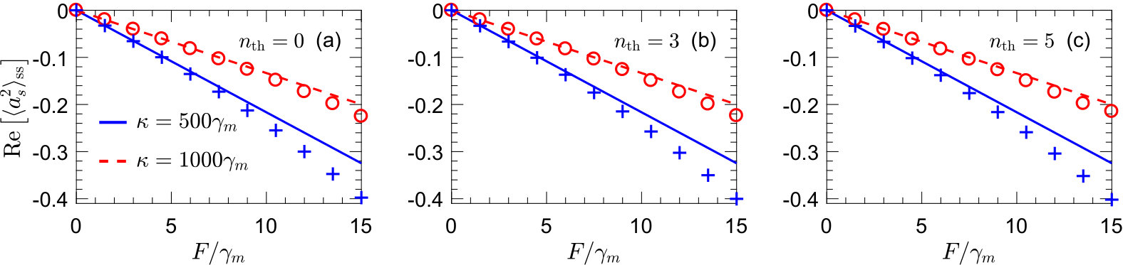 Figure 10
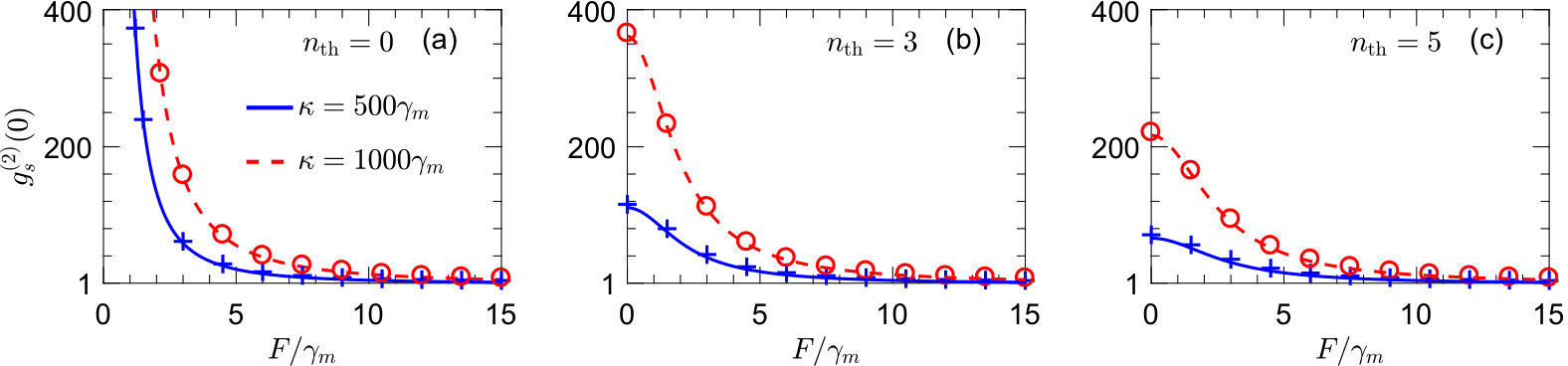 Figure 11
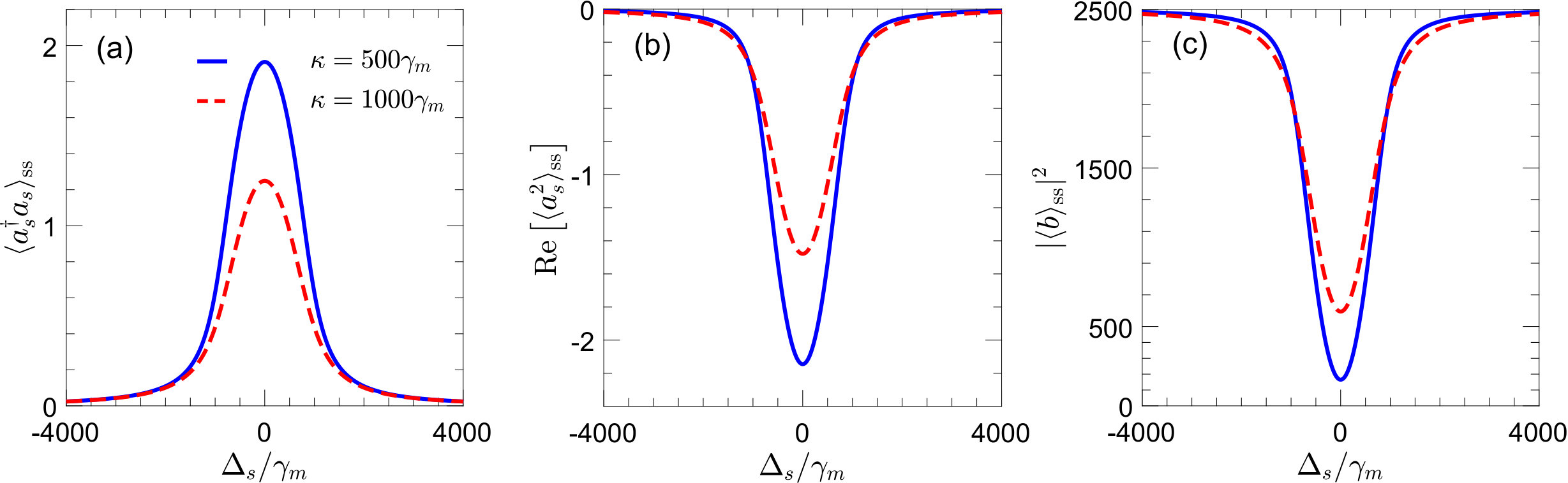 Figure 12
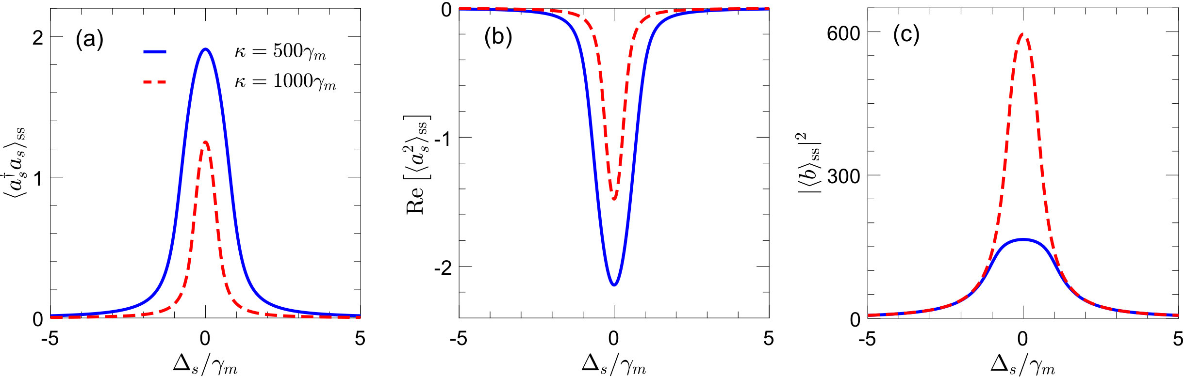 Figure 13
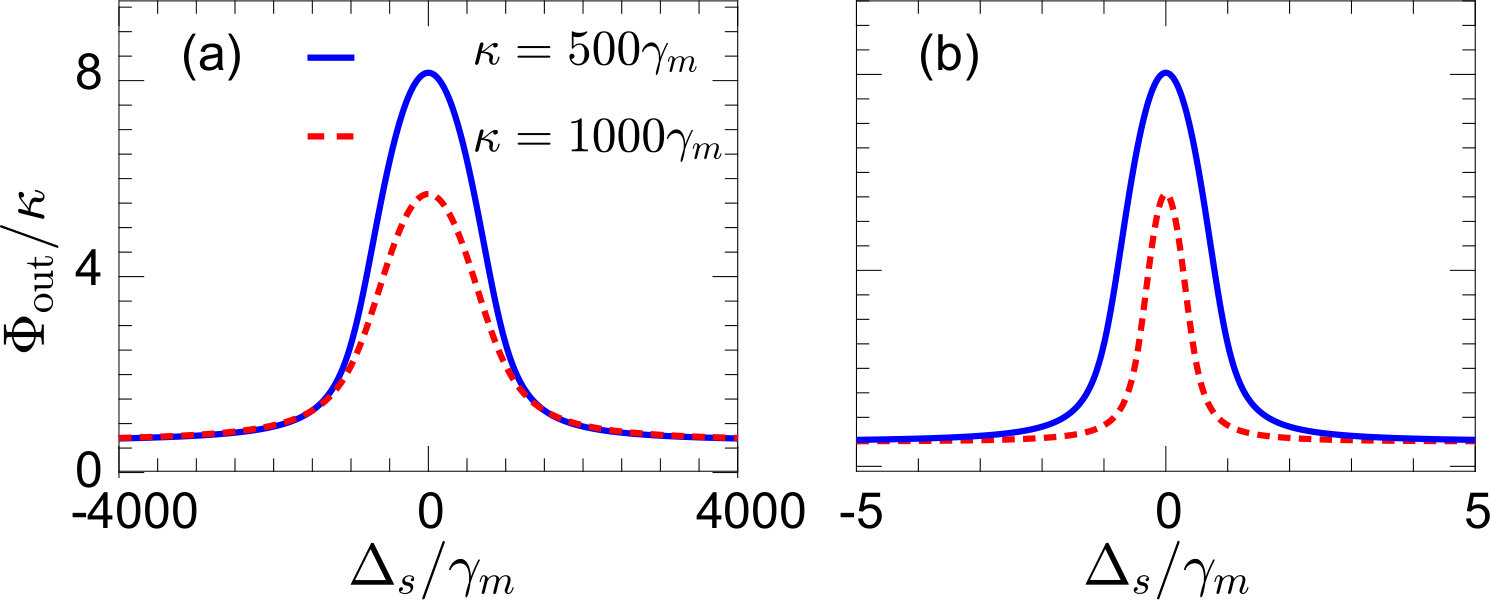 Figure 14
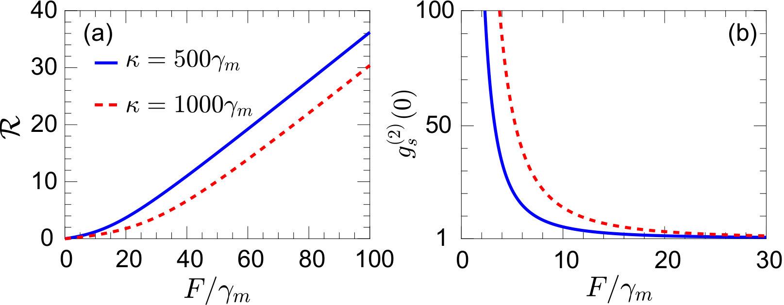 Figure 15
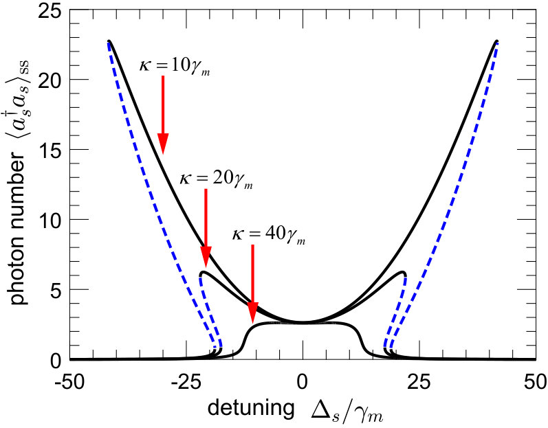 Figure 16
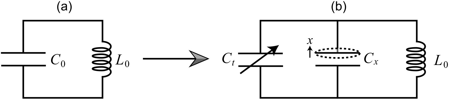 Figure 17
Peer Reviews
No public reviews on file for this paper yet. If you reviewed it on a platform where reviews are public (OpenReview, ICLR, NeurIPS, ICML), you can paste yours below so the community can read it here.
Videos
No videos yet. Explain this paper in a talk, walkthrough, or lecture? Add one.
Emission of photon pairs by mechanical stimulation of the squeezed vacuum
Wei Qin
Theoretical Quantum Physics Laboratory, RIKEN Cluster for Pioneering Research, Wako-shi, Saitama 351-0198, Japan
Vincenzo Macrì
Theoretical Quantum Physics Laboratory, RIKEN Cluster for Pioneering Research, Wako-shi, Saitama 351-0198, Japan
Adam Miranowicz
Theoretical Quantum Physics Laboratory, RIKEN Cluster for Pioneering Research, Wako-shi, Saitama 351-0198, Japan
Faculty of Physics, Adam Mickiewicz University, 61-614 Poznań, Poland
Salvatore Savasta
Theoretical Quantum Physics Laboratory, RIKEN Cluster for Pioneering Research, Wako-shi, Saitama 351-0198, Japan
Dipartimento di Scienze Matematiche e Informatiche, Scienze Fisiche e Scienze della Terra,
Università di Messina, I-98166 Messina, Italy
Franco Nori
Theoretical Quantum Physics Laboratory, RIKEN Cluster for Pioneering Research, Wako-shi, Saitama 351-0198, Japan
Department of Physics, The University of Michigan, Ann Arbor, Michigan 48109-1040, USA
Abstract
To observe the dynamical Casimir effect (DCE) induced by a moving mirror is a long-standing challenge because the mirror velocity needs to approach the speed of light. Here, we present an experimentally feasible method for observing this mechanical DCE in an optomechanical system. It employs a detuned, parametric driving to squeeze a cavity mode, so that the mechanical mode, with a typical resonance frequency, can parametrically and resonantly couple to the squeezed cavity mode, thus leading to a resonantly amplified DCE in the squeezed frame. The DCE process can be interpreted as mechanically-induced two-photon hyper-Raman scattering in the laboratory frame. Specifically, a photon pair of the parametric driving absorbs a single phonon and then is scattered into an anti-Stokes sideband. We also find that the squeezing, which additionally induces and amplifies the DCE, can be extremely small. Our method requires neither an ultra-high mechanical-oscillation frequency (i.e., a mirror moving at nearly the speed of light) nor an ultrastrong single-photon optomechanical coupling and, thus, could be implemented in a wide range of physical systems.
I Introduction
One of the most astonishing phenomena of nature, predicted by quantum field theory, is that the quantum vacuum is not empty but teems with virtual particles. Under certain conditions, these vacuum fluctuations could be converted into real particles by dynamical amplification mechanisms such as the Schwinger process Schwinger (1951), Hawking radiation Hawking (1974), and Unruh effect Unruh (1976). The dynamical Casimir effect (DCE) describes the creation of photons out of the quantum vacuum due to a moving mirror Moore (1970); Fulling and Davies (1976). The physics underlying the DCE is that the electromagnetic field cannot adiabatically adapt to the time-dependent boundary condition imposed by the mechanical motion of the mirror, such that it occurs a mismatch of vacuum modes in time. This gives rise to the emission of photon pairs from the vacuum and, at the same time, to the equal-energy dissipation of the mechanical phonons. Thus, according to energy conservation, the DCE can also be understood as the energy conversion of the mechanical motion to the electromagnetic field.
In order to detect the DCE, the mirror velocity is, however, required to be close to the speed of light Dodonov (2010); Nation et al. (2012). This requirement is the main obstacle in observing the DCE. This problem led to many alternative proposals, which replaced the mechanical motion with an effective motion provided by, e.g., modulating dielectric properties of semiconductors or superconductors Yablonovitch (1989); Lozovik et al. (1995); Crocce et al. (2004); Braggio et al. (2005); Segev et al. (2007), modulating the ultrastrong light-matter coupling in cavity quantum electrodynamics (QED) Ciuti et al. (2005); De Liberato et al. (2007, 2009); Garziano et al. (2013); Hagenmüller (2016); De Liberato (2017); Cirio et al. (2017); de Melo e Souza et al. (2018); Kockum et al. (2019); Forn-Díaz et al. (2019), or driving an optical parametric oscillator Dezael and Lambrecht (2010). In particular, two remarkable experimental verifications have recently been implemented utilizing a superconducting quantum interference device Nation et al. (2012); Johansson et al. (2009, 2010); Wilson et al. (2011); Dalvit (2011); Johansson et al. (2013a) and a Josephson metamaterial Lähteenmäki et al. (2013), respectively, to produce the effective motion. Despite such achievements, implementing the DCE with a massive mechanical mirror is still highly desirable for a more fundamental understanding of the DCE physics. This is because the parametric conversion of mechanical energy to photons, which is a key feature of the DCE predicted in its original proposals Moore (1970); Fulling and Davies (1976); Dodonov (2010); Nation et al. (2012), can be demonstrated in this case, contrary to proposals based on the effective motion. However, owing to the serious problem mentioned above (i.e., very fast oscillating mirror), such a radiation has not yet been observed experimentally, although the DCE has been predicted for almost fifty years. Here, we propose a novel approach to this outstanding problem, and we show that in a squeezed optomechanical system, a mirror oscillating at a common frequency can induce an observable DCE.
The DCE can, in principle, also be directly implemented in cavity-optomechanical systems Lambrecht et al. (1996); Dodonov and Klimov (1996); Plunien et al. (2000); Schaller et al. (2002); Kim et al. (2006); De Castro et al. (2013); Macrì et al. (2018); Sanz et al. (2018); Wang et al. (2019); Settineri et al. (2019). But it requires a mechanical frequency to be very close to the cavity frequency , or even a single-photon optomechanical coupling to reach the ultrastrong-coupling regime Macrì et al. (2018); Settineri et al. (2019). For typical parameters, MHz is much smaller than THz ( GHz) for optical (microwave) cavities, and at the same time, achieving the ultrastrong coupling is, currently, also a very challenging task in optomechanical experiments. However, as we describe in this manuscript, when squeezing the cavity Scully and Zubairy (1997), the squeezed-cavity-mode (SCM) frequency is tunable, such that the SCM can parametrically and resonantly couple to a mechanical mode with a typically available . This enables an observable DCE in the squeezed frame. Such a mechanical DCE corresponds to two-photon hyper-Raman scattering in the laboratory frame. Compared to one-photon Raman scattering typically demonstrated in cavity optomechanics, this hyper-Raman scattering process describes a photon pair scattered into a higher energy mode by absorbing a mechanical phonon.
As opposed to previous mechanical-DCE proposals, our approach requires neither an ultra-high mechanical frequency nor an ultrastrong coupling. In addition, the model discussed here is a generic optomechanical setup. Hence, with current technologies our proposal could be realized in various physical architectures, e.g., superconducting resonators Xiang et al. (2013); Gu et al. (2017) and optical cavities Reiserer and Rempe (2015). Furthermore, our proposal also shows mechanically-induced two-photon hyper-Raman scattering, which, to our knowledge, has not been considered before in cavity optomechanics.
II Model
We consider an optomechanical system, as schematically depicted in Fig. 1(a). The basic idea underlying our proposal is to use a detuned two-photon driving, e.g., of frequency and amplitude , to squeeze the cavity mode. The driving results in parametric down conversion of mechanical phonons to correlated cavity-photon pairs, which corresponds to the DCE. Furthermore, the SCM frequency completely depends on the detuning and the amplitude . This can be exploited to tune the parametric phonon-photon coupling into resonance, determining a strong amplification of the DCE. When the mechanical mode is driven, e.g., at frequency and amplitude , a strong steady-state output-photon flux that is induced by the DCE can be achieved.
To be specific, we consider the Hamiltonian
[TABLE]
Here,
[TABLE]
describes a standard optomechanical coupling,
[TABLE]
a detuned two-photon cavity driving, and
[TABLE]
a single-phonon mechanical driving. The bare cavity mode , when parametrically driven, is squeezed with a squeezing parameter
[TABLE]
and accordingly, is transformed to a squeezed mode , via the Bogoliubov transformation Scully and Zubairy (1997)
[TABLE]
Similar methods have been used for enhancing light-matter interactions in cavity optomechanics Lü et al. (2015); Lemonde et al. (2016) and cavity QED Qin et al. (2018); Leroux et al. (2018), but involving markedly different physical processes. As a result, is diagonalized to , where is a controllable SCM frequency. The optomechanical-coupling Hamiltonian is transformed, in terms of , to
[TABLE]
where is an effective single-photon optomechanical coupling, and is a coupling associated with the DCE. The dynamics under describes a mechanical modulation of the boundary condition of the squeezed field Law (1995); Macrì et al. (2018); Di Stefano et al. (2019). Under the rotating-wave approximation, the coherent dynamics of the system is governed by an effective Hamiltonian,
[TABLE]
where and . We find that when , the resonant DCE can be demonstrated, and that the parametric energy conversion of the mechanical motion to the electromagnetic field, which was predicted in the original DCE proposals, can therefore be observed. We also find that the energy of emitted photons in the squeezed frame completely originates from the mechanical motion. Thus, parametrically driving the cavity without a moving mirror Dezael and Lambrecht (2010), corresponding to , cannot excite the mode and cannot result in such a parametric energy conversion from mechanics to light.
III Mechanically-induced two-photon hyper-Raman scattering
More interestingly, the DCE in the squeezed frame can be interpreted, in the laboratory frame, as mechanically-induced two-photon hyper-Raman scattering. This hyper-Raman scattering is an anti-Stokes process, as illustrated in Fig. 1(b). According to the Bogoliubov transformation, the squeezing gives rise to an anti-Stokes sideband at frequency [right arrow in Fig. 1(b)]. The two-photon driving at frequency produces photon pairs at frequency [left arrow in Fig. 1(b)]. When mechanical phonons at frequency are present, a driving photon pair is scattered into the anti-Stokes sideband, while simultaneously absorbing a phonon in the mechanical resonator. Because of their different frequency from the driving photon pairs, the anti-Stokes scattered photon pairs, which are referred to as the DCE photons, can be spectrally filtered from the driving photons, which are referred to as the noise photons.
In cavity optomechanics, most of the experimental and theoretical studies are carried out under detuned one-photon driving of a cavity, so that the cavity field can be split into an average coherent amplitude and a fluctuating term. For a red-detuned driving, a driving photon can be scattered into the cavity resonance by absorbing a phonon. This process is viewed as mechanically-induced one-photon Raman scattering [dashed arrows in Fig. 1(c)]. As described above, our proposal instead exploits a red-detuned two-photon driving, and the mechanical motion can induce two-photon hyper-Raman scattering. In order to compare the two scattering processes more explicitly, we consider the limit . In this limit, the mode can be approximated by the mode, i.e., , and as a result, the anti-Stokes sideband becomes the cavity resonance. Correspondingly, the effective Hamiltonian becomes
[TABLE]
Under the resonant condition (i.e., 2), the dynamics described by shows that a driving photon pair, rather than a single photon, is scattered into the cavity resonance by absorbing a phonon [solid arrows in Fig. 1(c)].
IV How to observe the dynamical Casimir effect
In our approach, we squeeze the mode to make the effective cavity frequency very close to the mechanical frequency. However, this squeezing also inputs thermal noise and two-photon correlation noise into the cavity. Although these undesired effects are negligible in the weak-squeezing case (see below), they can be completely eliminated by coupling a squeezed-vacuum bath, e.g., with a squeezing parameter and a reference phase , to the mode Murch et al. (2013); Bartkowiak et al. (2014); Clark et al. (2017); Zeytinoğlu et al. (2017); Vahlbruch et al. (2018). We assume that and (), so that the mode is equivalently coupled to a vacuum bath (see Appendix A). The full dynamics is therefore determined by the standard master equation
[TABLE]
where and are the cavity and mechanical loss rates, respectively, and we have defined
[TABLE]
We have also assumed that the mechanical resonator is coupled to a zero-temperature bath (see Appendix B for an analytical discussion at finite temperatures). The SCM excitation spectrum , where \mbox{\langle o\rangle}_{\rm ss} represents a steady-state average value, is plotted in Figs. 2(a) and 2(b). Eliminating the squeezing-induced noise ensures a zero background noise for the excitation spectrum. If the mechanical resonator is driven, then photons are excited from the vacuum, and according to energy conservation, are emitted from the mechanical resonator, together with a resonance peak in the excitation spectrum.
We now return to the original laboratory frame and consider the steady-state output-photon flux. Because of the squeezing, the steady-state intracavity photon number, \mbox{\langle a^{{\dagger}}a\rangle}_{\rm ss}, in the laboratory frame includes two physical contributions, i.e.,
[TABLE]
where is the number of background-noise photons contained in the squeezed vacuum, and
[TABLE]
is the number of DCE-induced photons. The output-photon flux is then given by
[TABLE]
according to the input-output relation. We plot the flux spectrum in Figs. 2(c) and 2(d). There exists a nonzero background noise in the photon flux spectrum, as discussed previously. Nevertheless, when driving the mechanical resonator, the DCE-induced photons are emitted from the cavity, and a resolved resonance peak can be observed. We find that the behavior of the flux spectrum directly reflects that of the excitation spectrum. Hence, the emergence of the resonance peak in the flux spectrum can be considered as an experimentally observable signature of the DCE.
Owing to the existence of the background noise in the flux , we now discuss the ability to resolve the DCE signal from the background noise at resonance . In order to quantify this, we typically employ the signal-to-noise ratio, defined as
[TABLE]
The signal-resolved regime often requires , allowing for a resolved DCE-signal detection. We find that, by increasing the mechanical driving , the signal becomes stronger, but at the same time, the noise remains unchanged. This enables an improvement in the signal-to-noise ratio with the mechanical force. Consequently, the desired signal can be directly driven from the unresolved to resolved regime, as shown in Fig. 3(a). Assuming a realistic parameter , we find that a mechanical driving of is able to keep the ratio above for . With these parameters, we can obtain \mbox{\langle a_{s}^{{\dagger}}a_{s}\rangle}_{\rm ss}\approx 0.2, as given in Fig. 2. Therefore, in the laboratory frame, a cavity having a typical linewidth of MHz could emit photons per second, which is larger than the background photon emission per second. The ratio can be made as long as the driving is further increased, so that the background noise can be even neglected compared to the DCE signal. This is demonstrated in Appendix C, where we make a semi-classical approximation for investigating the DCE under a strong- drive. For
[TABLE]
the system behaves classically Wilson et al. (2010); Butera and Carusotto (2019), and quantum effects are negligible. Thus in order to observe the DCE, such a regime needs to be avoided. Note, however, that the signal can still be resolved even for , if standard techniques of Raman spectroscopy are used. This is because the background noise is due to driving photons at frequency , while the DCE photons have a frequency . The monotonic increase of the flux at resonance with the driving can, therefore, be considered as another signature of the mechanical DCE in experiments.
The DCE photons are emitted in pairs, and could exhibit photon bunching Johansson et al. (2010); Macrì et al. (2018); Stassi et al. (2013). The essential parameter characterizing this property is the equal-time second-order correlation function,
[TABLE]
We plot it as a function of the mechanical driving in Fig. 3(b). We find that
[TABLE]
in the limit, and in the limit (see Appendix B and C). Hence, for a weak- drive, the very small \mbox{\langle a_{s}^{{\dagger}}a_{s}\rangle}_{\rm ss} leads to . This corresponds to strong photon bunching. In the special case of , the mode cannot be excited although the two-photon driving still exists, and as a consequence, the correlation cannot be observed. We also find that with increasing the driving , the correlation decreases and then, as suggested above, approaches its lower bound equal to . These features confirm that the photons are bunched, as required.
So far, we have assumed a model with a squeezed-vacuum bath. To avoid using such a bath and simplify the model, we now consider the limit of . In this limit, the effective Hamiltonian is , as given above. In the absence of the squeezed-vacuum bath, the mode is coupled to a vacuum bath, and the master equation is the same as given in Eq. (10), but with . We find that the noise induced by squeezing the cavity, which includes thermal noise and two-photon correlation noise , becomes strongly suppressed, even when there is no squeezed-vacuum bath. The DCE dynamics of the simplified model is therefore similar to what we have already demonstrated for the model that includes a squeezed-vacuum bath. Such a similarity can be made closer by decreasing the ratio , but at the expense of the DCE radiation strength. In the limit of , the background noise is , so that all the photons radiated from the cavity can be thought of as the DCE photons. For realistic parameters , and , we could obtain \mbox{\langle a^{{\dagger}}a\rangle}_{\rm ss}\approx 1.8\times 10^{-3} at resonance (). This results in an output flux photons per second for MHz. This radiation can be measured using single-photon detectors.
V Possible implementations
As an example, we consider an LC superconducting circuit with a micromechanical membrane (see Appendix D for details). In this device, the LC circuit is used to form a single-mode microwave cavity. The mechanical motion of the membrane modulates the capacitance of the LC circuit, and thus the cavity frequency. In order to squeeze the cavity mode, an additional tunable capacitor is embedded into the device. Its cosine-wave modulation serves as a two-photon driving for the cavity mode. The squeezed-vacuum reservoir can be generated through an LC circuit with a tunable capacitor, or through a Josephson parametric amplifier Murch et al. (2013); Toyli et al. (2016).
Alternatively, our proposal can be implemented in an optical system such as a whispering-gallery-mode (WGM) microresonator coupled to a mechanical breathing mode Kippenberg et al. (2005); Schliesser et al. (2006); Fiore et al. (2011); Dong et al. (2012); Verhagen et al. (2012); Shen et al. (2016); Monifi et al. (2016). The WGM microresonator made from nonlinear crystals exhibits strong optical nonlinearities Fürst et al. (2011); Sedlmeir et al. (2017); Trainor et al. (2018), which is the essential requirement for squeezing. The squeezed-vacuum reservoir for the optical cavity can be prepared by pumping a nonlinear medium, e.g., periodically-poled (PPKTP) crystal, in a cavity Ast et al. (2013); Serikawa et al. (2016); Vahlbruch et al. (2016); Schnabel (2017).
VI Conclusions
We have introduced a method for how to observe the mechanical DCE in an optomechanical system. The method eliminates the problematic need for an extremely high mechanical-oscillation frequency and an ultrastrong single-photon optomechanical coupling. Thus, it paves an experimentally feasible path to observing quantum radiation from a moving mirror. Our method can be interpreted in the laboratory frame as mechanically-induced two-photon hyper-Raman scattering, an anti-Stokes process of scattering a driving photon pair into a higher energy mode by absorbing a phonon. For the absorbed phonon, its annihilation indicates the creation of a real photon pair out of the quantum vacuum in the squeezed frame. We have also showed a surprising result: that the squeezing, which additionally induces and amplifies the DCE, can be extremely weak. Note that in this case, the unconventional DCE can be considered somehow similar to unconventional photon blockade (UPB) Flayac and Savona (2017). Indeed, UPB is induced by a nonlinearity, which can be extremely small. Finally, we expect that the approach presented here could find diverse applications in theoretical and experimental studies of quantum vacuum radiation.
Acknowledgements.
S.S. acknowledges the Army Research Office (ARO) (Grant No. W911NF1910065). F.N. is supported in part by the: MURI Center for Dynamic Magneto-Optics via the Air Force Office of Scientific Research (AFOSR) (FA9550-14-1-0040), Army Research Office (ARO) (Grant No. Grant No. W911NF-18-1-0358), Asian Office of Aerospace Research and Development (AOARD) (Grant No. FA2386-18-1-4045), Japan Science and Technology Agency (JST) (via the Q-LEAP program, and the CREST Grant No. JPMJCR1676), Japan Society for the Promotion of Science (JSPS) (JSPS-RFBR Grant No. 17-52-50023, and JSPS-FWO Grant No. VS.059.18N), the RIKEN-AIST Challenge Research Fund, the Foundational Questions Institute (FQXi), and the NTT PHI Labs.
APPENDICES
Appendix A Optomechanical master equation, effective Hamiltonian, and off-resonant signal-to-noise ratio
A.1 Optomechanical master equation
In order to evaluate the steady-state behavior of the system, its interaction with the environment needs to be described carefully. In our proposal for observing the DCE, we parametrically squeeze the cavity mode. Related methods have been used to enhance the light-matter interaction in optomechanical systems Lü et al. (2015); Lemonde et al. (2016) and in cavity electrodynamics systems Qin et al. (2018); Leroux et al. (2018). This can make the squeezed-cavity-mode (SCM) frequency comparable to the mechanical frequency, so that the mechanically induced DCE can be observed in a common optomechanical setup without the need for an ultra-high mechanical frequency and an ultrastrong single-photon optomechanical coupling. However, the squeezing can also introduce undesired noise, including thermal noise and two-photon correlation, into the cavity. We can remove them by coupling a squeezed-vacuum bath to the bare-cavity mode. In this section, we give a detailed derivation of the master equation when the bare-cavity mode is coupled to a squeezed-vacuum bath and the mechanical mode is coupled to a thermal bath. We show that the noise induced by squeezing the cavity can be completely eliminated.
To begin with, we consider the Hamiltonian for the interaction between the system and the baths, which is given by
[TABLE]
where
[TABLE]
Here, is the free Hamiltonian of the baths, with the annihilation operators for the cavity and mechanical bath modes of frequency , and represent the couplings of the cavity and the mechanical resonator to their baths, with the coupling strengths depending on the frequency . To derive the master equation, we first switch into the frame rotating at
[TABLE]
to introduce the SCM using the Bogoliubov transformation . Then, we again switch into the frame rotating at , with being the SCM frequency, where is the detuning between the bare-cavity frequency and the half-frequency, , of the two-photon driving, and is the two-photon driving amplitude. The couplings between the system and the baths are, accordingly, transformed to
[TABLE]
Here, we have defined
[TABLE]
Following the standard procedure in Ref. Scully and Zubairy (1997) and, then, returning to the frame rotating at , we can obtain the following master equation expressed, in terms of the mode, as
[TABLE]
where the Lindblad superoperators are defined by
[TABLE]
and , are given, respectively, by
[TABLE]
corresponding to the thermal noise and two-photon correlation, and where
[TABLE]
represent, respectively, the cavity and mechanical decay rates, with being the density of states for the cavity bath at frequency , and being the density of states for the mechanical bath at frequency . Moreover, is the equilibrium phonon occupation at temperature .
Note that, to derive the master equation in Eq. (A.1), we have assumed that the central frequency of the squeezed-vacuum bath is equal to half the two-photon driving frequency. In addition, we have made the following approximations,
[TABLE]
This is because, in our case, the SCM frequency is tuned to be comparable to the mechanical frequency ( MHz). Thus, it is much smaller than the two-photon driving frequency (of the order of GHz for microwave light or even THz for optical light).
According to Eqs. (A.1) and (A.1), we can have for and (), and thus, we have,
[TABLE]
We find from Eq. (A.1) that the squeezing-induced noise is completely eliminated, so that the mode is equivalently coupled to the thermal vacuum bath. As we demonstrate below, eliminating this noise can ensure that the background noise is zero for the SCM excitation spectrum in the squeezed frame, and as a result, the background noise of the output-photon flux spectrum in the original laboratory frame only originates from photons contained in the squeezed vacuum. This minimizes the background noise for the observation of the DCE, and thus enables the DCE to be observed more clearly in experiments.
When the conditions and () are not perfectly satisfied, the squeezing-induced noise cannot be eliminated completely (i.e., and ). However, according to the master equation in Eq. (A.1), such imperfections do not affect the occurrence of the DCE. They only cause some noises. To quantify this undesired effect, we use the signal-to-noise ratio defined as
[TABLE]
where () is the steady state when (), and the subscript “ss” stands for “steady state”. We plot in Fig. A1, according to the master equation given in Eq. (A.1) but replacing . In this figure, we assume that and . In the perfect case of , because . Thus, we find in Fig. A1 that the noise induced by imperfect parameters reduces the ratio . However, we also find that with increasing the driving , the noise becomes smaller compared to the DCE signal, such that it can even be neglected for sufficiently strong .
A.2 Effective Hamiltonian
The Hamiltonian in Eqs. (A.1) and (A.1) is expressed, in terms of the mode, as
[TABLE]
where and , with being the squeezing parameter of the cavity. In Fig. A2(a) we plot as a function of and , and find that the resonance condition , for a parametric coupling between SCM and mechanical mode, can be achieved with experimentally modest parameters. The Hamiltonian essentially describes the optomechanical system where the boundary condition of a squeezed field is modulated by the mechanical motion of a driven mirror. In the limit , we can apply the rotating-wave approximation, such that the coherent dynamics of the system is governed by the following effective Hamiltonian,
[TABLE]
where and . The master equation in Eq. (A.1) is then reduced to
[TABLE]
We find, according to Eq. (A.2), that the coupling of the states and , where the first number in the ket refers to the SCM photon number and the second one to the mechanical phonon number, is given by
[TABLE]
In the squeezed frame, this means that under the time evolution, one phonon can be converted into two photons, and vice versa, at resonance . To confirm such a state conversion, we perform numerics, as shown in Fig. A2(b). Specifically, we use the master equation in Eq. (A.1) to calculate the fidelity, , where is the actual state. It is seen in Fig. A2(b) that we have the expected state conversion between light and mechanics, and there is a maximum conversion at resonance. Note that owing to the presence of the cavity and mechanical losses, the maximum conversion fidelity decreases with time.
To describe the dynamics of the DCE further, we plotted the time evolution of in the presence of the driving in Fig. A3. We find that increases with time and then gradually approaches its stationary value. For an experimental parameter Hz in Ref. Teufel et al. (2011), the stationary state is reached within a time ms.
In Eq. (A.2), we made the rotating-wave approximation and neglected the high-frequency component
[TABLE]
In typical situations, , which allows a time-averaging treatment of using the formalism of Ref. Gamel and James (2010). After a straightforward calculation, the behavior of can be approximated, at resonance (i.e., ), as
[TABLE]
The Hamiltonian is, accordingly, transformed to
[TABLE]
For realistic parameters, the couplings and are three orders of magnitude lower than . We can find from Eq. (A.2) that the high-frequency term can be neglected, compared to the low-frequency term . To confirm this, in Fig. A4 we numerically calculated using the low-frequency term and the full Hamiltonian given in Eq. (29), respectively. By comparing these, we find an excellent agreement, and the high-frequency term can be safely neglected, as expected.
A.3 Off-resonant signal-to-noise ratio
In the main article, the signal-to-noise ratio is discussed at resonance (i.e., ). We now discuss the ratio in the off-resonance case where and . We plot the ratio as a function of the detunings and in Fig. A5. There, the results are obtained by numerically integrating the master equation in Eq. (A.2). We find that the ratio decreases with the detuning or , but increases with the force . Note that the DCE photons are the scattered photon pairs via two-photon hyper-Raman scattering. As a result, their frequency is different from the noise-photon frequency . This means that if standard techniques of Raman spectroscopy are used, the noise can then be filtered out. Therefore, the signal can still be resolved even if .
Appendix B Dynamical Casimir effect in the mechanical weak-driving regime
In our main article, we have studied the steady-state behavior associated with the DCE, by numerically integrating the master equation in Eq. (A.2) Johansson et al. (2012, 2013b). To study the DCE further, an analytical understanding for the mechanical weak driving is given in this section. Here, we only focus on the resonance situation where .
Let us now derive the steady-state SCM photon number . To begin, we consider the master equation in Eq. (A.2). The involved equations of motion are given, respectively, by
[TABLE]
Here, represents the imaginary part of . In fact, owing to the parametric coupling, the Hamiltonian in Eq. (A.2) leads to an infinite set of differential equations, which may not be analytically solved. Thus, in order to obtain an analytical result, we neglect the higher-order correlation terms, that is: , , , , and . This approximation is valid for a weak driving , as shown below. In such an approximation, the coupled differential equations (30)–(B) construct a closed set, so in the steady state we have
[TABLE]
By solving this closed set of equations, the steady-state SCM photon number is found to be
[TABLE]
where . Equation (42) shows that \mbox{\langle a_{s}^{{\dagger}}a_{s}\rangle}_{\rm ss} includes two physical contributions: one from the mechanical driving and the other from the thermal noise. Furthermore, we also find a quadratic increase in \mbox{\langle a_{s}^{{\dagger}}a_{s}\rangle}_{\rm ss} with the driving . To confirm this analytical expression, in Fig. A6 we compare it with exact numerical simulations of the master equation in Eq. (A.2). It is seen that the analytical predictions are in good agreement with the exact numerical results, especially for weak .
According to the Bogoliubov transformation, the steady-state intracavity-photon number \mbox{\langle a^{{\dagger}}a\rangle}_{\rm ss} in the original laboratory frame is given in Eq. (12). Then, the steady-state output-photon flux is given in Eq. (14).
To obtain analytically, the physical quantities \mbox{\langle a_{s}^{{\dagger}}a_{s}\rangle}_{\rm ss} and {\rm Re}\left[\mbox{\langle a_{s}^{2}\rangle}_{\rm ss}\right] are involved, as shown in Eq. (13). The steady-state SCM photon number, \mbox{\langle a_{s}^{{\dagger}}a_{s}\rangle}_{\rm ss}, is given in Eq. (42), and further is numerically confirmed in Fig. A6. From the closed set of the steady-state equations given in Eqs. (36)–(41), we can straightforwardly find
[TABLE]
It shows that |{\rm Re}\left[\mbox{\langle a_{s}^{2}\rangle}_{\rm ss}\right]| increases linearly with but is independent of the thermal mechanical noise. This behavior is also numerically confirmed in Fig. A7, showing a good agreement especially for the weak driving . Note that the derivation of the analytical results and their numerical confirmations originates from neglecting the higher-order correlation terms. In order to exactly describe , such higher-order correlations should be included. By combining Eqs. (42)–(43), the steady-state output-photon flux can be analytically expressed as
[TABLE]
We find from Eq. (B) that, by increasing the mechanical driving , the DCE-induced photon flux becomes stronger quadratically, but at the same time, the background-noise photon flux remains unchanged. Therefore, the increase in the total photon flux with can be considered as a signature of the mechanical-motion induced DCE.
In the DCE process, the photons are emitted in pairs, and therefore, they could exhibit photon bunching Johansson et al. (2010); Stassi et al. (2013); Macrì et al. (2018). The essential parameter quantifying this property is the equal-time second-order correlation function, defined in Eq. (17). We now derive this second-order correlation function. The equation of motion for is given by
[TABLE]
We can neglect the term {\rm Im}\left[\mbox{\langle a_{s}^{{\dagger}}a_{s}^{3}b^{{\dagger}}\rangle}\right] for the weak driving . Then, combining Eq. (36) yields
[TABLE]
In Fig. A8, we plot the correlation as a function of the driving . In this figure, we compare the analytical and numerical results, and show an exact agreement. Owing to a very small of \mbox{\langle a_{s}^{{\dagger}}a_{s}\rangle}_{\rm ss} for the mechanical weak driving, is very large as shown in Fig. A8, which corresponds to large photon bunching. With increasing the driving , we also find that the correlation decreases, and as demonstrated more explicitly in the Appendix C, it would approach a lower bound equal to , thereby implying that the DCE radiation field becomes a coherent state in the limit of the mechanical strong driving, .
Appendix C Semi-classical treatment for the dynamical Casimir effect
In Appendix B we have analytically discussed the DCE process when the mechanical driving is weak. There, the higher-order correlations that arise from the parametric coupling are neglected, and the resulting expressions can predict the system behavior well. For strong- driving, all high-order correlations should be included to exactly describe the system; but in this case, finding solutions analytically or even numerically becomes much more difficult. In order to investigate the DCE in the strong- regime, in this section we employ a semi-classical treatment Butera and Carusotto (2019). For simplicity, but without loss of generality, here we assume that the mechanical resonator is coupled to a zero-temperature bath. For finite temperatures, the discussion below is still valid, as long as the total number of phonons is much larger than the number of thermal phonons.
C.1 Excitation spectrum and output-photon flux spectrum in the steady state
We again begin with the master equation in Eq. (A.2) and, accordingly, obtain
[TABLE]
Here, we have made the semiclassical approximation, such that \mbox{\langle a_{s}^{2}b^{{\dagger}}\rangle}\approx\mbox{\langle a_{s}^{2}\rangle}\mbox{\langle b\rangle}^{*} and \mbox{\langle a_{s}^{{\dagger}}a_{s}b\rangle}\approx\mbox{\langle a_{s}^{{\dagger}}a_{s}\rangle}\mbox{\langle b\rangle}. Under this approximation, the fluctuation correlation between the cavity and the mechanical resonator is neglected. It is found that Eqs. (47)–(49) construct a closed set.
C.1.1 Excitation spectrum for resonant mechanical driving:
We first consider the case of a resonant mechanical driving (i.e., ). In this case, we have , and the steady-state SCM photon number \mbox{\langle a_{s}^{{\dagger}}a_{s}\rangle}_{\rm ss} satisfies a cubic equation,
[TABLE]
where and x=2\mbox{\langle a_{s}^{{\dagger}}a_{s}\rangle}_{\rm ss}+1. The solutions of such a equation can be exactly obtained using the Cardano formula. Then, the steady-state and are given, respectively, by
[TABLE]
For simplicity, we numerically solve the cubic equation (C.1.1), and in Fig. A9 we plot \mbox{\langle a_{s}^{{\dagger}}a_{s}\rangle}_{\rm ss}, {\rm Re}\left[\mbox{\langle a_{s}^{2}\rangle}_{\rm ss}\right], and |\mbox{\langle b\rangle}_{\rm ss}|^{2} versus the detuning for and . At large detunings, the resonantly driven mechanical resonator is effectively decoupled from the cavity mode. As a consequence, there is almost no conversion of mechanical energy into photons. Thus at large detunings, the mechanical phonon number |\mbox{\langle b\rangle}_{\rm ss}|^{2} quickly approaches , i.e., the steady-state phonon number when the mechanical resonator is completely uncoupled. Meanwhile, both the photon number \mbox{\langle a_{s}^{{\dagger}}a_{s}\rangle}_{\rm ss} and correlation function \mbox{\langle a_{s}^{2}\rangle}_{\rm ss} are very close to zero. As the detuning decreases, the effective parametric coupling between the mechanical motion and the cavity mode increases, and the parametric conversion from mechanical energy into photons is accordingly enhanced. Such an energy conversion is maximized at resonance . Thus, when decreasing the detuning, both \mbox{\langle a_{s}^{{\dagger}}a_{s}\rangle}_{\rm ss} and |{\rm Re}\left[\mbox{\langle a_{s}^{2}\rangle}_{\rm ss}\right]| increase but |\mbox{\langle b\rangle}_{\rm ss}|^{2} decreases, as shown in Fig. A9. In particular, \mbox{\langle a_{s}^{{\dagger}}a_{s}\rangle}_{\rm ss} and |{\rm Re}\left[\mbox{\langle a_{s}^{2}\rangle}_{\rm ss}\right]| reach their maximum values at resonance, and at the same time, |\mbox{\langle b\rangle}_{\rm ss}|^{2} reaches its minimum value. This behavior implies that the photons are emitted by the mechanical resonator.
C.1.2 Excitation spectrum for resonant parametric coupling:
We next consider the case of a resonant parametric coupling (i.e., ). In this case, we have , and the steady-state also satisfies a cubic equation
[TABLE]
where . This cubic equation can also be exactly solved using the Cardano formula, and then the steady-state and are given, respectively, by
[TABLE]
We numerically solve the cubic equation (C.1.2), and in Fig. A10, we plot \mbox{\langle a_{s}^{{\dagger}}a_{s}\rangle}_{\rm ss}, {\rm Re}\left[\mbox{\langle a_{s}^{2}\rangle}_{\rm ss}\right], and |\mbox{\langle b\rangle}_{\rm ss}|^{2} versus the detuning for and . At large detunings, the mechanical driving is effectively decoupled from the mechanical resonator, so that almost no phonons are excited and almost no photons are emitted. As the detuning decreases, the mechanical phonon number increases, which strengthens the parametric conversion from mechanical energy into photons, and in turn, leads to an increase in the excited photon number. This process is maximized at resonance . Thus, we find, as shown in Fig. A10, that with decreasing the detuning, not only \mbox{\langle a_{s}^{{\dagger}}a_{s}\rangle}_{\rm ss} and |{\rm Re}\left[\mbox{\langle a_{s}^{2}\rangle}_{\rm ss}\right]| but also |\mbox{\langle b\rangle}_{\rm ss}|^{2} increases, and that they simultaneously reach their maximum values at resonance. This behavior also implies that the photons are emitted by the mechanical resonator.
C.1.3 Output-photon flux spectrum for resonant mechanical driving and parametric coupling
Having obtained \mbox{\langle a_{s}^{{\dagger}}a_{s}\rangle}_{\rm ss} and \mbox{\langle a_{s}^{2}\rangle}_{\rm ss} in the squeezed frame, we can, according to the Bogoliubov transformation, calculate the steady-state intracavity photon number \mbox{\langle a^{{\dagger}}a\rangle}_{\rm ss} in the original laboratory frame, as given in Eq. (12). Then we can calculate the steady-state output-photon flux according to the input-output relation, given in Eq. (14). We plot the photon flux as a function of the detuning in Fig. A11. As expected, for a given mechanical driving, we can observe a resonance peak, corresponding to the maximum value of the photon flux. This behavior in the laboratory frame can directly reflect the behavior of the excitation spectrum \mbox{\langle a_{s}^{{\dagger}}a_{s}\rangle}_{\rm ss}\left(\Delta_{s}\right) in the squeezed frame in Figs. A9(a) and A10(a). This is because the background noise remains unchanged when the detuning is changed, and the peak completely arises from the DCE in the squeezed frame. Thus, the appearance of the peak of the output flux spectrum can be considered as an experimentally observable signature of the DCE.
C.2 Signal-to-noise ratio and second-order correlation function at resonance
As mentioned before, there exists a background noise in the flux . Thus, we need to analyze the ability of our proposal to resolve the DCE-induced signal from the background noise. To quantitatively describe this ability, we typically employ the signal-to-noise ratio defined in Eq. (15). Without loss of generality, we focus on the ratio at resonance . Under this resonance condition, the cubic equation satisfied by \mbox{\langle a_{s}^{{\dagger}}a_{s}\rangle}_{\rm ss} becomes
[TABLE]
where x=2\mbox{\langle a_{s}^{{\dagger}}a_{s}\rangle}+1. Then, \mbox{\langle a_{s}^{2}\rangle}_{\rm ss} and \mbox{\langle b\rangle}_{\rm ss} are given by
[TABLE]
We plot the ratio versus the driving in Fig. A12(a). We find that the signal-to-noise ratio monotonically increases with the mechanical driving. This is owing to the fact that an increase in the mechanical driving leads to an increase in the number of DCE-induced photons, but at the same time leaves the number of background-noise photons unchanged.
The equal-time second-order correlation function is defined in Eq. (17). Similarly to the discussion of the signal-to-noise ratio , we also only focus on the correlation at resonance . In the semi-classical treatment presented in this section, \mbox{\langle a_{s}^{{\dagger}2}a_{s}^{2}\rangle}_{\rm ss} can be approximated as \mbox{\langle a_{s}^{{\dagger}2}a_{s}^{2}\rangle}_{\rm ss}\approx|\mbox{\langle a_{s}^{2}\rangle}_{\rm ss}|^{2}, and as a result, the correlation is reduced to
[TABLE]
which is plotted as a function of the mechanical driving in Fig. A12(b). We find that starts with very large values, and as the mechanical driving increases, then decreases approaching 1. This behavior, as expected, suggests the phenomenon of photon bunching, thus confirming the DCE.
C.3 Analytical solutions in the limits and
In order to have a better analytical understanding, let us now consider the limit of , and also the opposite limit of , at resonance .
For the limit, we have \mbox{\langle a_{s}^{{\dagger}}a_{s}\rangle}_{\rm ss}\rightarrow 0, and thus, x^{n}\approx 1+2n\mbox{\langle a_{s}^{{\dagger}}a_{s}\rangle} for . Based on this, an approximate solution of the cubic equation in Eq. (C.2) is found to be
[TABLE]
which corresponds to Eq. (42) for . Analogously, we obtain
[TABLE]
Note that Eq. (61) corresponds to Eq. (43). Therefore, according to Eq. (B), we obtain a quadratic increase in the ratio
[TABLE]
with large driving , as shown in Fig. A12(a).
In the opposite limit of , we have x\rightarrow 2\mbox{\langle a_{s}^{{\dagger}}a_{s}\rangle}_{\rm ss}, and then obtain
[TABLE]
Consequently, the photon flux is given by
[TABLE]
This indicates a linear increase in the ratio with the driving , as shown in Fig. A12(a).
For the correlation in the limit of , we find
[TABLE]
which is the same as Eq. (46). This corresponds to a large as in Fig. A12(b) and, thus, to large photon bunching.
Furthermore, in the opposite limit of , the correlation function is approximately equal to , i.e.,
[TABLE]
as shown Fig. A12(b). This means that the DCE radiation field is approximately in a coherent state.
C.4 Stability analysis
We now turn to multistability effects of our system. As discussed previously, in the semi-classical approximation, the system is governed by a cubic function. However, a cubic function has three solutions, and thus the system may exhibit multistability effects. To analyze them, we need to perform steady-state analysis Sarchi et al. (2008). Thus, we express the quantities , , and as the sum of their steady-state values (\mbox{\langle a_{s}^{{\dagger}}a_{s}\rangle}_{\rm ss}, \mbox{\langle a_{s}^{2}\rangle}_{\rm ss}, \mbox{\langle b\rangle}_{\rm ss}) and time-dependent small perturbations [, , ], that is,
[TABLE]
Then, substituting these equations into Eqs. (47), (C.1), and (49) yields
[TABLE]
We further make the following replacements,
[TABLE]
where and () are time-independent complex numbers, and denotes a complex frequency. Then, the coupled equations (C.4), (C.4), and (75) can be rewritten as
[TABLE]
where
[TABLE]
[TABLE]
where
[TABLE]
If all imaginary parts of the eigenvalues of the matrix are negative, then the system is stable; otherwise the system is unstable Kyriienko et al. (2014). According to this criterion, we estimate the stability of our system. We find that for the parameters used in the above discussion about the DCE, the system does not exhibit multistability. Furthermore, when the mechanical loss is close to the cavity loss, we find for that the system becomes multistable, as shown in Fig. A13. However, the requirement that the mechanical loss is close to the cavity loss makes the threshold
[TABLE]
very low. For , the system behaves classically, and quantum effects are negligible Wilson et al. (2010); Butera and Carusotto (2019). For the parameters in Fig. A13, the value of is (here, we set ), which is smaller than one fifth of the force . As a consequence, the system, when demonstrating such multistable behaviors, has probably reached the classical regime, where the DCE effect induced by the quantum fluctuations is negligible. Therefore, in order to observe the DCE, it is better to avoid the multistable regime of the system.
Appendix D Possible implementations with superconducting quantum circuits
Our scheme to implement the DCE is based on a generic optomechanical system, and at the same time, does not require an ultra-high-frequency mechanical resonator and an ultrastrong single-photon coupling between light and mechanical motion. Therefore, we can expect that it can be implemented in various physical systems. In this section, as an example, we discuss in detail a possible implementation with superconducting circuits and, in particular, we refer to the experimental superconducting quantum circuit of Ref. Teufel et al. (2011), described by the standard optomechanical coupling of the form .
A standard LC circuit consists of a capacitor (e.g., with capacitance ) and an inductor (e.g., with inductance ), as shown in Fig. A14(a). Its Hamiltonian is expressed in terms of the capacitor charge and the inductor current as
[TABLE]
where is the magnetic flux through the inductor, and is the fundamental frequency of the circuit. After quantization, the charge and the flux represent a pair of canonically conjugate variables, which obey the commutation relation . Upon introducing a canonical transformation,
[TABLE]
the Hamiltonian becomes
[TABLE]
Here, we have subtracted the constant zero-point energy . Such an LC circuit thus behaves as a single-mode microwave cavity, with being the cavity frequency, and with () being the annihilation (creation) operator of the cavity mode.
As demonstrated in Ref. Teufel et al. (2011), when the capacitance in Fig. A14(a) is modulated by the mechanical motion of a micromechanical membrane, the mechanical motion can couple to the cavity mode. In this manner, the capacitance becomes
[TABLE]
where is the displacement of the membrane, and is the distance between the conductive plates of the capacitor. To parametrically squeeze the cavity mode, we further add an additional and electrically tunable capacitor into such an experimental setup. The LC circuit is shown in Fig. A14(b). Here, we assume the capacitance of the additional capacitor to be
[TABLE]
where is the modulation frequency, and . The total capacitance is thus given by . Note that, in the absence of both mechanical motion and cosine modulation, the total capacitance is equal to , and as a result, the resonance frequency of the bare LC cavity, shown in Fig. A14(b), is , rather than . When both mechanical motion and cosine modulation are present, the cavity frequency is modulated as
[TABLE]
In the limit , we can expand , up to first order, to have
[TABLE]
The Hamiltonian describing the cavity mode of the LC circuit in Fig. A14(b) is then given by
[TABLE]
Using the canonical transformation in Eq. (D), but with replaced by , the Hamiltonian is reduced to
[TABLE]
where () is the annihilation (creation) operator of the mechanical mode, is the single-photon optomechanical coupling, is the zero-point fluctuation of the mechanical resonator, is the amplitude of the two-photon driving, and is its frequency. Here, we have made the rotating-wave approximation, and we have also replaced
[TABLE]
After including the free Hamiltonian of the mechanical resonator, the full Hamiltonian, in a rotating frame at , becomes ()
[TABLE]
where is the frequency of the mechanical mode, and . The Hamiltonian in Eq. (D) is exactly the one applied by us in this work.
A squeezed-vacuum reservoir coupled to the cavity mode can be realized directly using the LC circuit in Fig. A14(a), but the constant capacitance needs to be replaced by a tunable capacitance . By following the same recipe as above, the corresponding Hamiltonian is then given by
[TABLE]
where , and . The canonical transformation used here is the same as given in Eq. (D). When the input field of the cavity is in the vacuum, we can obtain a squeezed-vacuum field at the output port, according to the input-output relation.
In addition to the LC circuit, the squeezed-vacuum reservoir can also be generated by a Josephson parametric amplifier, as experimentally demonstrated in Refs. Murch et al. (2013); Toyli et al. (2016). In particular, a squeezing bandwidth of up to MHz was reported in Ref. Murch et al. (2013). This is sufficient to fulfil the large-bandwidth requirement of the reservoir.
The reference list from the paper itself. Each links out to its DOI / PubMed record.
- 1Schwinger (1951) J. Schwinger, “On Gauge Invariance and Vacuum Polarization,” Phys. Rev. 82 , 664 (1951) .
- 2Hawking (1974) S. W. Hawking, “Black hole explosions?” Nature 248 , 30 (1974) . · doi ↗
- 3Unruh (1976) W. G. Unruh, “Notes on black-hole evaporation,” Phys. Rev. D 14 , 870 (1976) .
- 4Moore (1970) G. T. Moore, “Quantum Theory of the Electromagnetic Field in a Variable-Length One-Dimensional Cavity,” J. Math. Phys. 11 , 2679–2691 (1970) . · doi ↗
- 5Fulling and Davies (1976) S. A. Fulling and P. C. W. Davies, “Radiation from a moving mirror in two dimensional space-time: conformal anomaly,” Proc. R. Soc. Lond. A 348 , 393–414 (1976) .
- 6Dodonov (2010) V. V. Dodonov, “Current status of the dynamical Casimir effect,” Phys. Scr. 82 , 038105 (2010) .
- 7Nation et al. (2012) P. D. Nation, J. R. Johansson, M. P. Blencowe, and F. Nori, “Colloquium: Stimulating uncertainty: Amplifying the quantum vacuum with superconducting circuits,” Rev. Mod. Phys. 84 , 1 (2012) .
- 8Yablonovitch (1989) E. Yablonovitch, “Accelerating reference frame for electromagnetic waves in a rapidly growing plasma: Unruh-Davies-Fulling-Dewitt radiation and the nonadiabatic Casimir effect,” Phys. Rev. Lett. 62 , 1742 (1989) .