Particle filters for data assimilation based on reduced order data models
John Maclean, Erik S Van Vleck

TL;DR
This paper introduces a novel data assimilation framework using low-rank projections, specifically a projected Particle Filter, to improve high-dimensional state estimation by mitigating particle collapse.
Contribution
The paper develops a projected Particle Filter based on low-rank projections, compatible with any DA method, and demonstrates its effectiveness in high-dimensional problems.
Findings
Projected Particle Filter reduces particle collapse in high dimensions
The method preserves relevant information from unstable modes
Numerical comparisons show improved performance over standard filters
Abstract
We introduce a framework for Data Assimilation (DA) in which the data is split into multiple sets corresponding to low-rank projections of the state space. Algorithms are developed that assimilate some or all of the projected data, including an algorithm compatible with any generic DA method. The major application explored here is PROJ-PF, a projected Particle Filter. The PROJ-PF implementation assimilates highly informative but low-dimensional observations. The implementation considered here is based upon using projections corresponding to Assimilation in the Unstable Subspace (AUS). In the context of particle filtering, the projected approach mitigates the collapse of particle ensembles in high dimensional DA problems while preserving as much relevant information as possible, as the unstable and neutral modes correspond to the most uncertain model predictions. In particular we…
Click any figure to enlarge with its caption.
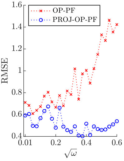 Figure 5
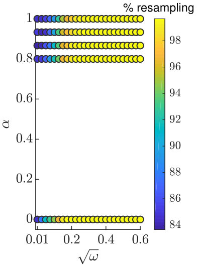 Figure 5
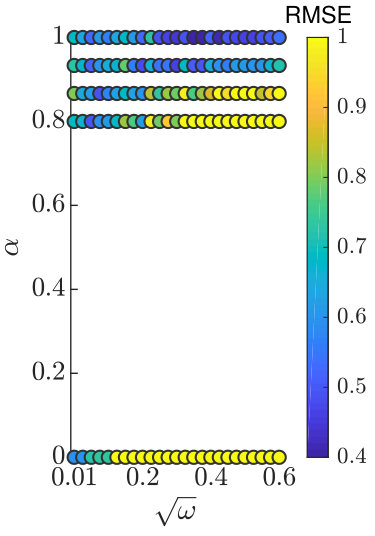 Figure 5
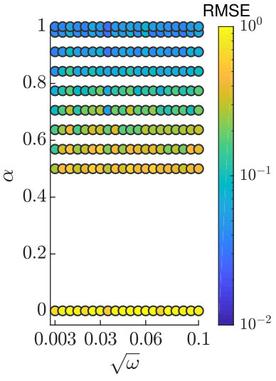 Figure 4
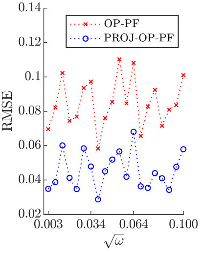 Figure 5
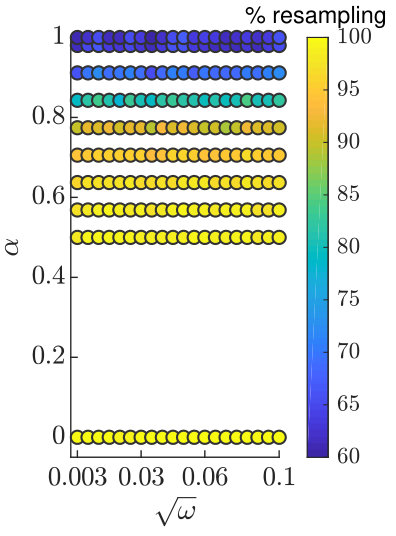 Figure 6
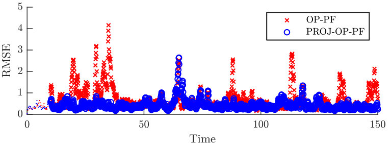 Figure 7
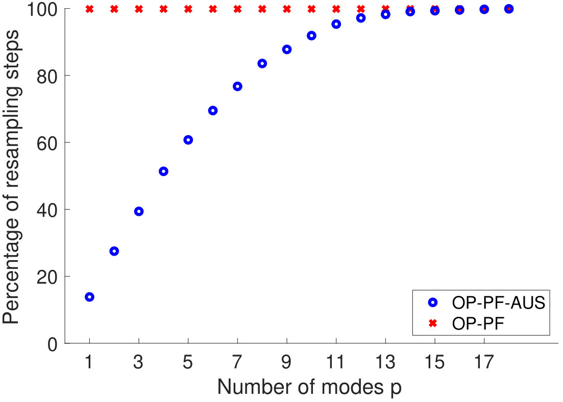 Figure 8
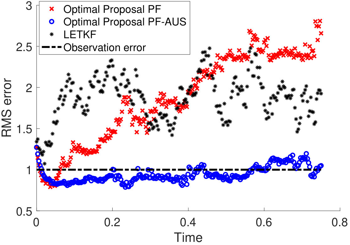 Figure 9
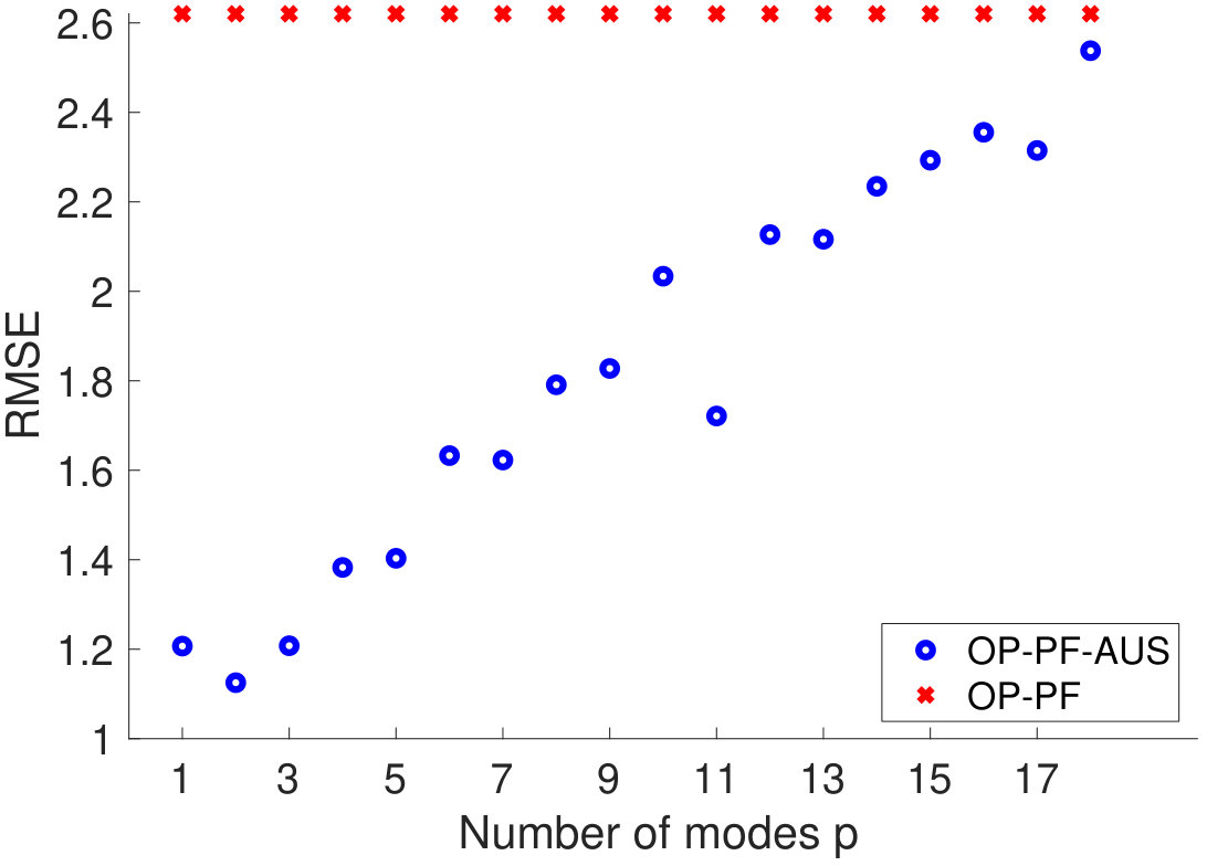 Figure 10
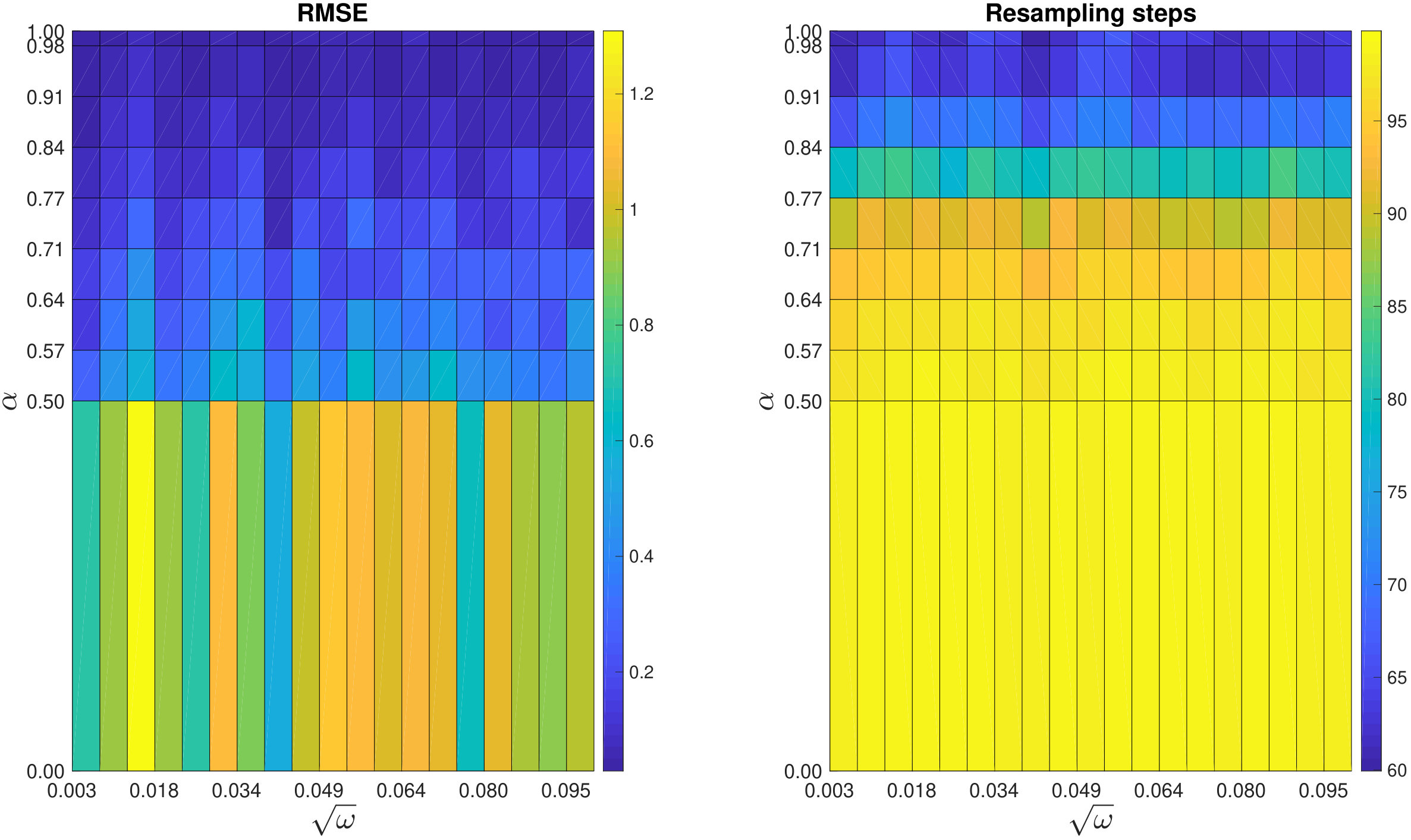 Figure 11
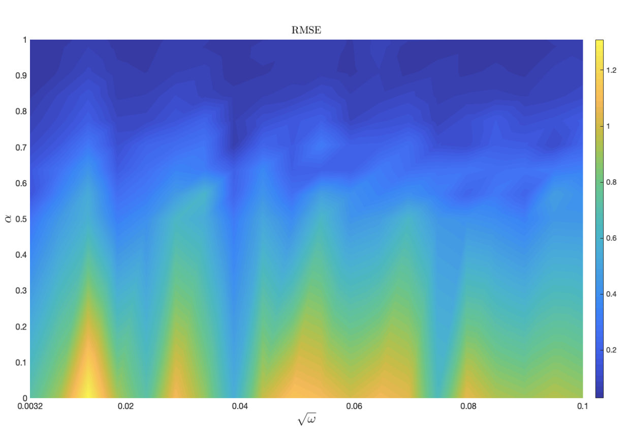 Figure 12
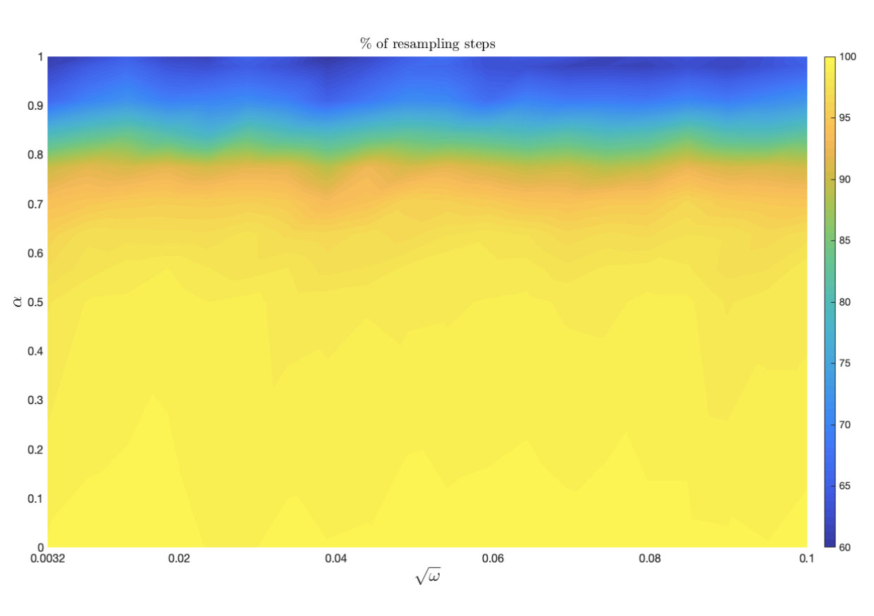 Figure 13
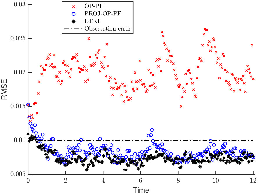 Figure 14
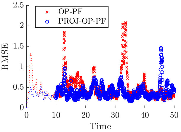 Figure 15
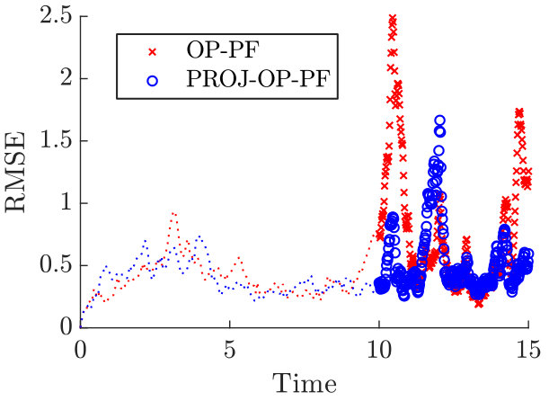 Figure 16
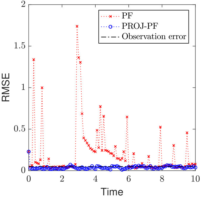 Figure 17
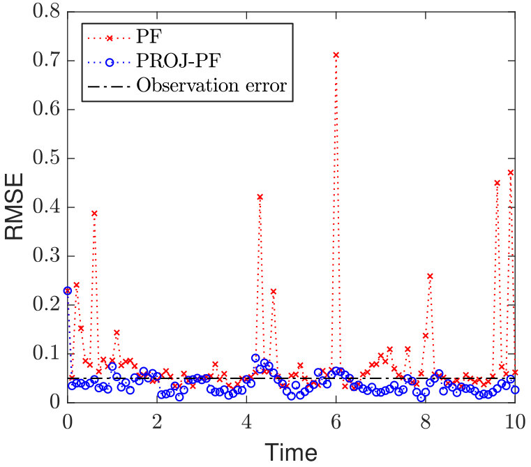 Figure 18
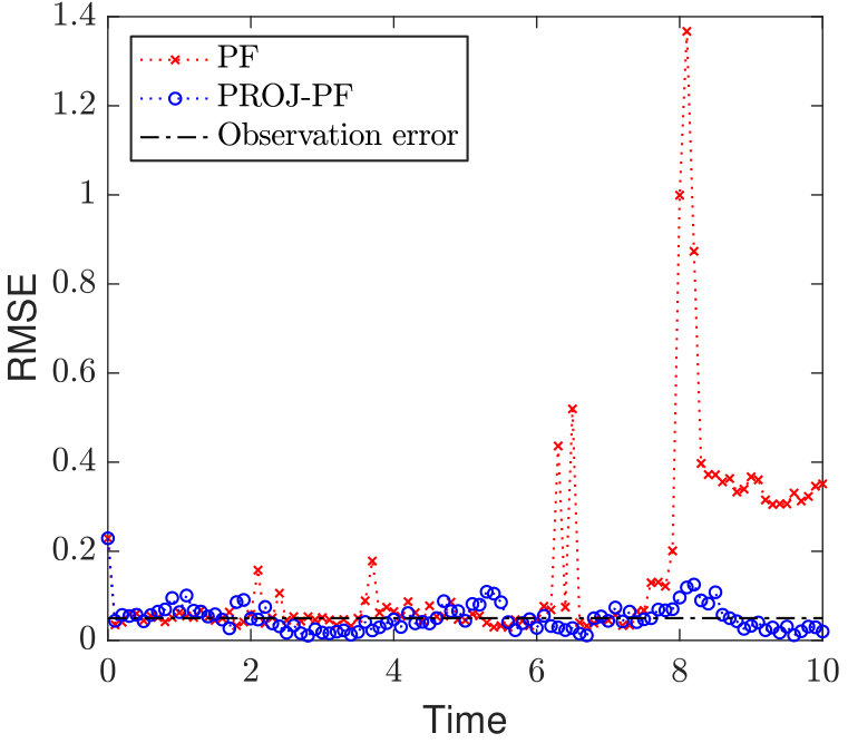 Figure 19
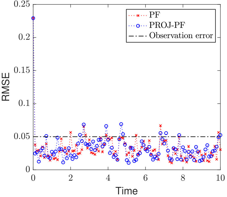 Figure 20
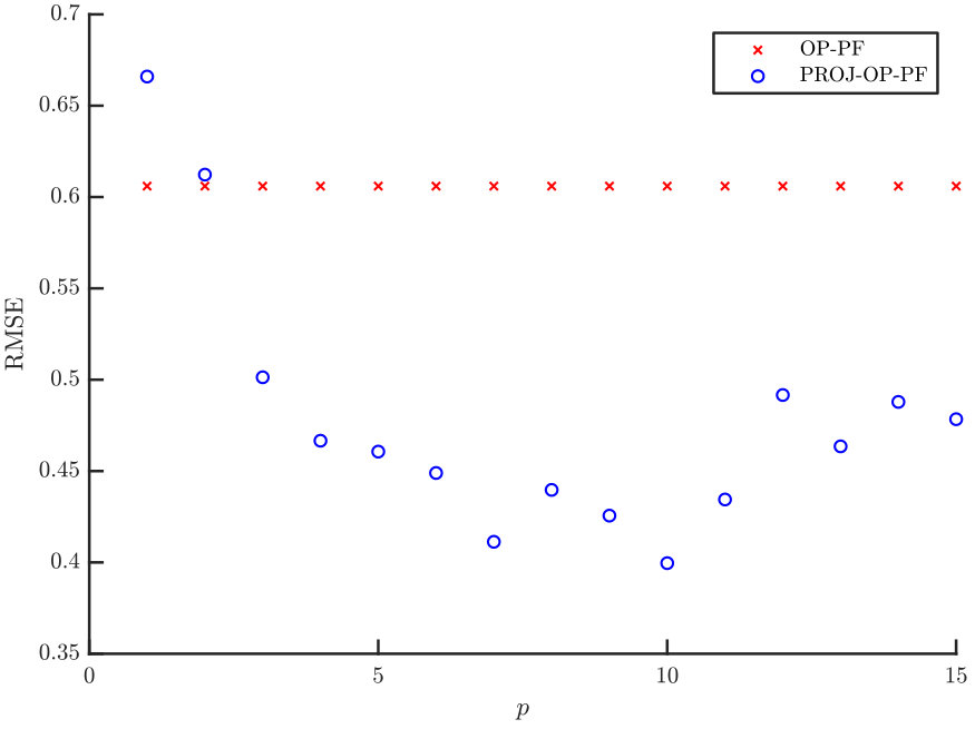 Figure 21
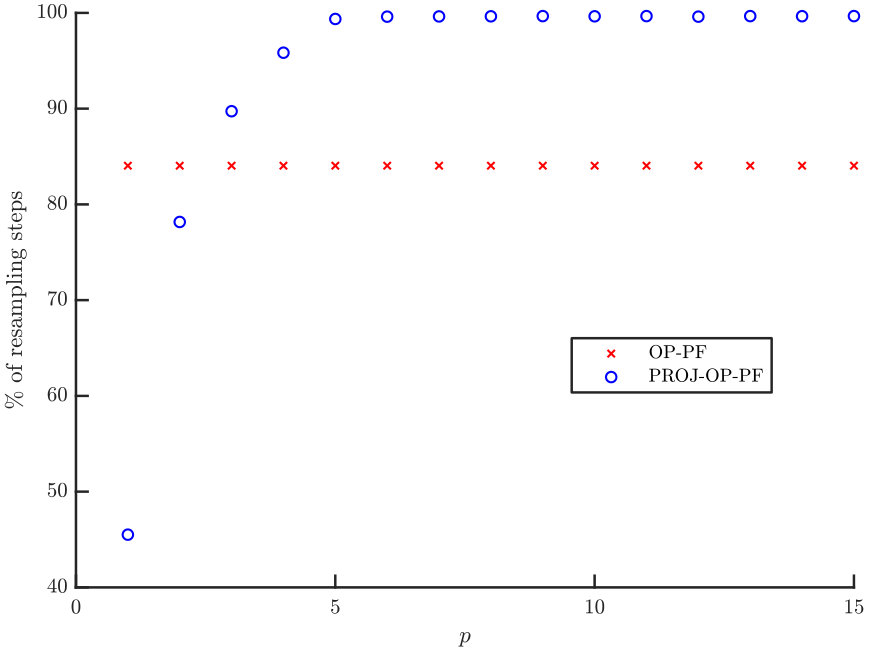 Figure 22
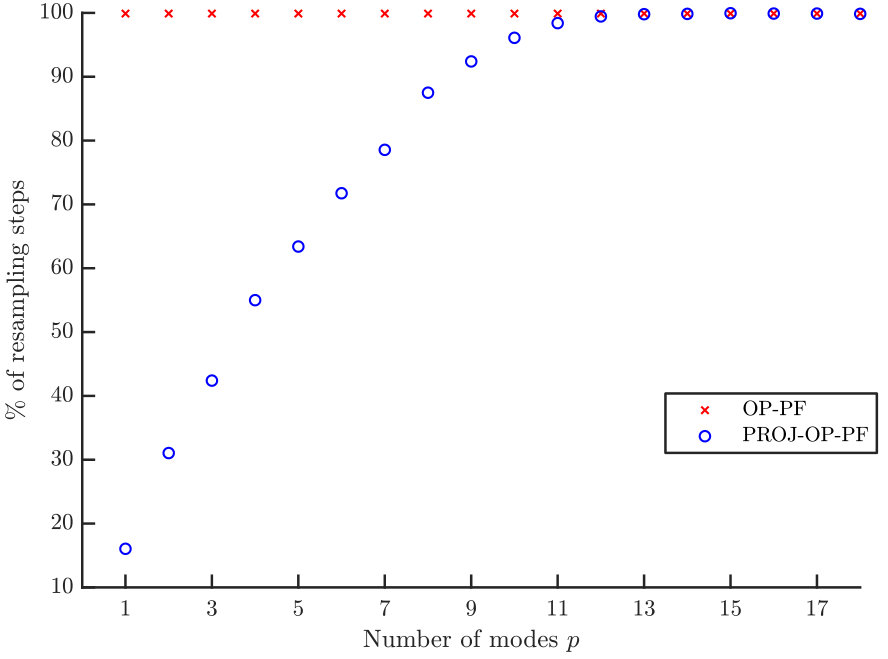 Figure 23
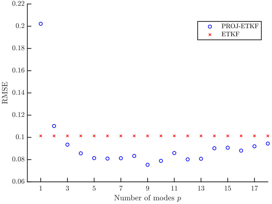 Figure 24
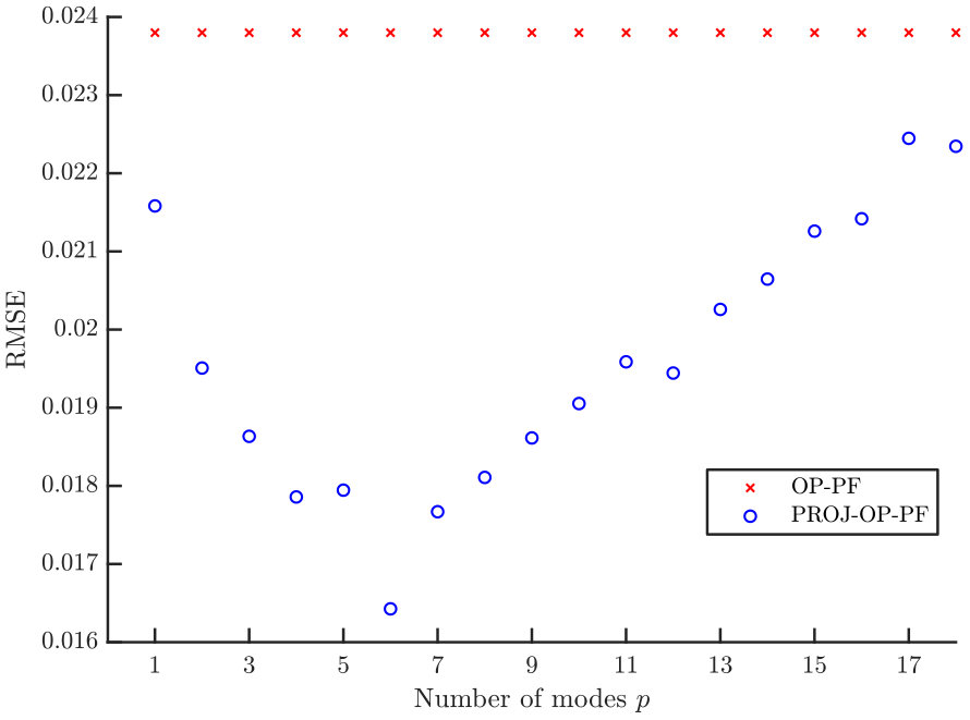 Figure 25
| 1 | 2 | 3 | 4 | 5 | 6 | 7 | 8 | 9 | 10 | 11 | 12 | 13 | 14 | 15 | |
|---|---|---|---|---|---|---|---|---|---|---|---|---|---|---|---|
| 0.01 | 0.13 | 0.13 | 0.13 | 0.20 | 0.20 | 0.20 | 0.20 | 0.15 | 0.13 | 0.20 | 0.07 | 0.13 | 0.07 | 0.13 |
Peer Reviews
No public reviews on file for this paper yet. If you reviewed it on a platform where reviews are public (OpenReview, ICLR, NeurIPS, ICML), you can paste yours below so the community can read it here.
Videos
No videos yet. Explain this paper in a talk, walkthrough, or lecture? Add one.
\runningheads
J.M. and E.V.V.Q. J. R. Meteorol. Soc.
\corraddr
Particle filters for data assimilation based on reduced order
data models222JM, ONR, grant: N00014-18-1-2204; ARC, grant DP180100050; EVV, NSF, DMS-1714195 and DMS-1722578.
John Maclean\corrauth
a
Erik S. Van Vleck
b
aaaffiliationmark: School of Mathematical Sciences, University of Adelaide, South Australia. http://www.adelaide.edu.au/directory/john.maclean
bbaffiliationmark: Department of Mathematics, University of Kansas, USA. http://people.ku.edu/~erikvv/
Abstract
We introduce a framework for Data Assimilation (DA) in which the data is split into multiple sets corresponding to low-rank projections of the state space. Algorithms are developed that assimilate some or all of the projected data, including an algorithm compatible with any generic DA method. The major application explored here is PROJ-PF, a projected Particle Filter. The PROJ-PF implementation assimilates highly informative but low-dimensional observations. The implementation considered here is based upon using projections corresponding to Assimilation in the Unstable Subspace (AUS). In the context of particle filtering, the projected approach mitigates the collapse of particle ensembles in high dimensional DA problems while preserving as much relevant information as possible, as the unstable and neutral modes correspond to the most uncertain model predictions. In particular we formulate and numerically implement a projected Optimal Proposal Particle Filter (PROJ-OP-PF) and compare to the standard optimal proposal and to the Ensemble Transform Kalman Filter.
keywords:
Data Assimilation, Numerical Analysis, Dimension Reduction
1 Introduction
Many data assimilation techniques were developed based on extending assumptions of linearity in the phase space and data models and under the assumption of Gaussian errors. Several techniques have proven to be successful in weakening these assumptions, while other techniques have been developed to explicitly overcome these obstacles. Important among these are particle filters (Doucet et al., 2000), a key subject of this paper. Particle filters have proven to be successful for low dimensional assimilation problems but tend to have difficulty with higher dimensional problems. Different variants of particle filters have been develop to combat these difficulties, including implicit particle filters, proposal density methods, the optimal proposal, etc (Chorin et al., 2010; Snyder et al., 2008; van Leeuwen, 2010; Snyder, 2011). Recent work has often focused on the issue of localization (Farchi and Bocquet (2018), e.g.), and two localised particle filtering algorithms (Poterjoy and Anderson, 2016; Potthast et al., 2019) have been applied in an operational geophysical framework. The localised particle filter of Potthast et al. (2019) contains an element related to the approach taken in this paper. In particular, in Potthast et al. (2019) observations are projected onto the subspace spanned by the ensemble of model forecasts. This is shown to effect a significant reduction in the dimension of the data, one which mitigates the issues that high model dimension induces in particle filters.
Our contribution in this paper is to develop a framework for data assimilation schemes in which the data are constrained by an arbitrary projection to lie in some subspace of observation or model space. We explicitly obtain a form for the reduction in data dimension, and an expression that determines how much the posterior of the Bayesian DA scheme is affected by use of the projection. While the projection is not specified, the key idea is that some physically based reduction technique can then be employed in concert with a DA scheme. In such a way the assimilation step is performed in a space of very low dimension. A cognate approach in Potthast et al. (2019) projects the data onto the subspace spanned by the forecast ensemble, originating in the Local Ensemble Transform Kalman Filter (Hunt et al., 2007).
The derivation in this paper was motivated in large part by assimilation in the unstable subspace (AUS) techniques. These techniques have largely focused on projecting the phase space model using Lyapunov vectors while employing the original data or observational model. The techniques and framework developed in this paper allow for combinations of (time dependent) projected and unprojected physical and data models, and their formulation is independent of the source of the projections. The framework and techniques lead to several natural applications. In particular we develop, implement, and compare two new particle filter algorithms based upon a dimension reduction technique into the unstable subspace.
We now discuss the historical antecedents of the projections in this manuscript, and connect them to other recent filtering approaches. The AUS techniques (Carrassi et al., 2008a; Trevisan et al., 2010; Palatella et al., 2013; Law et al., 2014; Sanz-Alonso and Stuart, 2015) to improve speed and reliability of data assimilation specifically address the partitioning of the tangent space into stable, neutral and unstable subspaces corresponding to Lyapunov vectors associated with negative, zero and positive Lyapunov exponents. In particular, Trevisan, d’Isidoro & Talagrand propose a modification of 4DVar, so-called 4DVar-AUS, in which corrections are applied only in the unstable and neutral subspaces (Trevisan et al., 2010; Palatella et al., 2013). These techniques are based on updating in the unstable portion of the tangent space and may be interpreted in terms of projecting covariance matrices during the assimilation step.
Motivated by these techniques for assimilation in the unstable subspace, in de Leeuw et al. (2018) a new method is developed for data assimilation that utilizes distinct treatments of the dynamics in the stable and non-stable directions. In particular, the first phase of this development has involved employing time dependent Lyapunov vectors to form a subsystem with tangent space dynamics similar to the unstable subspace of the original state space model. This was motivated by AUS techniques. The key piece of de Leeuw et al. (2018) related to this work is the following projected model update. For a smooth discrete time model and projection , and for any reference solution, solve for :
[TABLE]
This manuscript develops a complementary approach to project the data model. The two approaches will be compared in Section 5.1.
Another branch of projected DA schemes use the ‘Dynamically Orthogonal’ (DO) formulation (Sapsis and Lermusiaux, 2009; Sapsis, 2010), in which the forecast model is broken into a partial differential equation governing the mean field and a number of stochastic differential equations describing the evolution of components in a time-dependent stochastic subspace of the original differential equation. The DO approach was used to assimilate with different DA schemes in the subspace and mean field space in Sondergaard and Lermusiaux (2013); Majda et al. (2014); Qi and Majda (2015). These techniques use both a projected and mean field model to make a forecast, similar to using (1). The data is naturally split into the ‘projected’ and remaining components without using a projected data model (see, e.g., (15)) explicitly, as the data may be confined to the DO-subspace by simply subtracting the forecast mean field. This attractive feature of the DO methodology bypasses the need to derive a projected data model, as the covariance structure of the data does not change.
Projection-based DA schemes have been developed to assimilate coherent structures (Maclean et al., 2017) or features (Morzfeld et al., 2018) in the data. These approaches have used likelihood-free sequential Monte Carlo methods, or an ad hoc ‘perturbed observations’ approach, to deal with the difficulty of calculating the likelihood function for a coherent structure. The derivation in this paper may lead to an explicit likelihood for data-derived coherent structures/features obtained via a projection. Additional sources for projections may be found in the review of projection based model reduction techniques (Benner et al., 2015).
We develop a projected DA framework and algorithms for arbitrary time dependent orthogonal projections, but are mainly interested in the AUS approach where the projections identify the unstable/neutral subspace. To determine the projections we will employ standard techniques for approximation of Lyapunov exponents, e.g., the so-called discrete QR algorithm (see Dieci and Van Vleck (2007, 2015)).
Unlike most past work related to AUS our primary focus is on developing a systematic approach to confining the data, not the model, to the unstable subspace. In some of the initial works on AUS (Carrassi et al., 2007, 2008b), either target observations at the location where the unstable mode attains its maximum value, or only the observations falling in the vicinity of the maximum, were assimilated. Albeit empirical, that choice already signified using only data projected on an approximation of the unstable subspace, that was obtained by Breeding on the Data Assimilation Cycle (BDAS). Furthermore, González-Tokman and Hunt (2013); Bocquet et al. (2017); Grudzien et al. (2018a); Frank and Zhuk (2018) are all at least in part devoted to discussing the necessary and/or sufficient criteria for filter stability in terms of the projection of the observations into the unstable/neutral/weakly stable directions and this is directly related to the choice of adaptive observation operators in Law et al. (2014).
If the non-stable subspace is relatively low dimensional this makes applications of techniques such as particle filters appealing. Particle Filters (Doucet et al., 2001) are particularly effective for nonlinear problems and for the tracking of non-Gaussian, multi-modal probability distributions; but they suffer from the so-called curse of dimensionality (Snyder et al., 2008; Snyder, 2011; Morzfeld et al., 2012; Van Leeuwen, 2012, e.g.). There is a known formulation that minimises degeneracy; however, even with a linear model, it is known that the computational cost of this "Optimal Proposal" Particle Filter scales like the exponential of the observation dimension (Snyder, 2011). Our aim in this work is to avoid the established limits of particle filter performance by reducing the observation dimension in a sensible way. Other efforts to bypass this limitation include, e.g., the Equivalent Weights Particle Filter (van Leeuwen, 2010). One attractive feature of our approach is that it is a reformulation of the standard DA problem rather than a specific algorithm, and so it is compatible with these advanced particle filters.
The availability of the projection into the unstable subspace will also allow us to develop a novel approach to resampling. It is necessary to periodically refresh any particle ensemble, and some noise is usually added at this step. To avoid forcing the ensemble off the attractor with this added noise we confine most of the noise to the unstable subspace, which improves the filter accuracy and reduces the incidence of resampling in later steps.
This paper is organized as follows. Data assimilation is reviewed in section 2 and projected DA is formulated in section 3. Algorithms for using the new projected data are introduced (section 4) and applied to AUS with several numerical experiments (section 5). A discussion (section 6) and bibliography conclude the paper.
2 Data Assimilation
Data assimilation methods combine orbits from a dynamical system model with measurement data to obtain an improved estimate for the state of a physical system. In this paper we develop a data assimilation method in the context of the discrete time stochastic model
[TABLE]
where are the state variables at time and , i.e., drawn from a normal distribution with mean zero and model error covariance . Let the sequence , be a distinguished orbit of this system, referred to as the true solution of the model, and presumed to be unknown. As each time is reached we collect an observation related to via
[TABLE]
where , , is the observation operator, and the noise variables are drawn from a normal distribution with zero mean and known observational error covariance matrix . In general the observation operator can be nonlinear.
We formulate DA under the ubiquitous Bayesian approach. Consider the assimilation of a single observation, , at time step . Given a prior estimate of the state, Bayes’ Law gives
[TABLE]
Using (3) the likelihood function is, up to a normalization constant,
[TABLE]
This procedure, which we have written for the assimilation of data at a single observation time, readily extends to the sequential assimilation of observations at multiple times under the assumptions that the state is Markovian and the observations at different times are conditionally independent (see for example Budhiraja et al. (2017)).
In the following we introduce some key DA schemes. Not much detail is given here, but the interested reader is referred in particular to three recent books on DA, (Reich and Cotter, 2015; Law et al., 2015; Asch et al., 2016).
2.1 Kalman Filtering
The Kalman Filter and later extensions are ubiquitous in DA, and are now briefly described. For a linear model, i.e. where (2) is
[TABLE]
and for the linear observation operator , the Kalman Filter calculates the exact posterior , where the analysis variables are
[TABLE]
The weight matrix is the Kalman gain matrix
[TABLE]
The superscript is reserved for forecast variables, obtained at time by using (5) to update ,
[TABLE]
[TABLE]
Two extensions of the Kalman Filter are prevalent in nonlinear DA, the Extended Kalman Filter (EKF) and Ensemble Kalman Filter (EnKF). Neither give the exact posterior for a nonlinear model.
2.1.1 Extended Kalman Filter
The nonlinear model (2) is used to make the forecast , and then the Kalman Filter update is applied using the linearisation
[TABLE]
If the observation operator is a nonlinear function , the linearization
[TABLE]
is used everywhere except to compute the innovation in the calculation of .
The EKF is suitable for low dimensional nonlinear filtering, but the required linearizations are nontrivial for high-dimensional filtering. The EnKF by contrast is well suited to high dimensions.
2.1.2 Ensemble Kalman Filter
The Ensemble Kalman Filter is a Monte Carlo approximation of the Kalman Filter that is well suited to high dimensional filtering problems, introduced in Evensen (1994); Burgers et al. (1998). An ensemble of forecasts are made at time , from to . Then the forecast covariance is approximated by the sample covariance of the ensemble, and the analysis ensemble is obtained in such a way that its mean satisfies (6) and its sample covariance satisfies (7). In this paper we will use analysis updates corresponding to the Ensemble Transform Kalman Filter (ETKF) (Bishop et al., 2001).For more details and a modern introduction to the Ensemble Kalman Filter, see e.g. Evensen (2009).
2.2 The Particle Filter
Particle Filters (PF) are a collection of particle based data assimilation schemes that do not rely on linearization of the dynamics or Gaussian representations of the posterior; see Doucet et al. (2001) for a comprehensive review. The basic idea is to represent the prior distribution , previously the forecast, and the posterior distribution , previously the analysis, by discrete probability measures. Suppose that at time we have the posterior distribution , supported on points and with weights . Each and . Here L is the number of particles that are used to approximate the distribution . The two key steps in the Particle Filter are as follows:
Prediction step. Propagate each of the particles . One simple choice, the bootstrap PF, is to use the state dynamics (2) to forecast each particle.
This gives the forecast probability distribution as a discrete probability measure concentrated on points with weights .
Filtering step. Update the weights using the observation . In the bootstrap PF the update is
[TABLE]
where is chosen so that .
This scheme is easy to implement but suffers from severe degeneracy, especially in high dimensions. That is, after a few time steps all the weight tends to concentrate on a few particles. A common remedy is to monitor the Effective Sample Size (ESS) and resample when the ESS drops below some threshold in order to refresh the particle cloud; see e.g. Doucet et al. (2001); Budhiraja et al. (2017).
2.2.1 The Optimal Proposal
The optimal proposal particle filter (OP-PF) (Snyder et al., 2008; Doucet et al., 2000; Snyder, 2011; Van Leeuwen, 2012) attempts to address the degeneracy issue in particle filters with the aim of ensuring that all posterior particles have similar weights. The ‘proposal’ is the distribution used to update the particles from one time step to the next. In the prediction step in the basic particle filter above, the particles are updated using the model, so the proposal density in that approach is (compare (2)) .
The optimal proposal density is . Given the additive noise of the model (2), the optimal proposal update in each particle is Gaussian with , where
[TABLE]
The prefactor can be written as the Kalman gain (8) (albeit with ) by an application of the Sherman-Morrison-Woodbury formula (see e.g. Kalnay (2003), p. 171).
Two applications of Bayes’ law (e.g. in Snyder (2011)) show that the weight update for the -th particle drawn from this proposal satisfies and is also Gaussian,
[TABLE]
where .
As mentioned in the previous section, degeneracy - characterised by a single particle with weight of approximately - is a common problem in the PF. In Snyder et al. (2015) it is shown that, of all PF schemes that obtain using and , the ‘optimal proposal’ above has the minimum variance in the weights. That is, it suffers the least from weight degeneracy. In van Leeuwen et al. (2018) this result is extended to any PF scheme that obtains using , and .
The distributions required to apply the Optimal Proposal are not always available (the additive model error of (2) and linear observation operator of (3) are used above to obtain closed forms for the individual particle updates and weight updates), but when OP-PF can be formulated it is the least degenerate of a large class of filters. However, in Snyder (2011) it is shown that the optimal proposal requires an ensemble size L satisfying for a linear model, or will suffer from filter degeneracy. That is, filter degeneracy is intimately connected to model and observation dimension, and is a fundamental obstacle to Particle Filtering in high dimensional problems.
3 Projected Data Models
We now develop an approach to decompose the observations using projections defined in state space. A wealth of techniques from dynamical systems theory can then be used to obtain low-dimensional data models.
Suppose that at time a dynamically significant rank orthogonal projection is available, as well as data .
The main result will be to define a projected observation , and derive a corresponding data model
[TABLE]
that is a linear transformation of (3), where and are orthogonal projections with () and , and has known distribution. The projected data contains only the components of observations that can be written as a linear combination of the columns of . It can be used in place of the original data in any DA algorithm, or used in concert with the original data in the novel Particle Filtering algorithm developed in Section 4.
We will derive (12) in the following three steps.
Step One: lift the data into model space
In order to apply the projection to data, we first need to find an equivalent representation of the data in model space.
Assuming has full row rank, we define an -dimensional vector where . The data model for is
[TABLE]
where is an orthogonal projection, and .
Using that one readily confirms that . That is, the observation operator collapses onto the standard data model. The transformation through has not affected the output of a DA scheme, as ; however is of compatible dimension with .
Step Two: project the data into a rank subspace
We now make use of the orthogonal projection . The idea is to formulate a new data model, along the lines of , that contains only the components of the observation that align with the projection. The projected data models that are developed here may be considered as generalizations of the construction of observation operators (see Grudzien et al. (2018a) Def. 13 and Law et al. (2014)).
Define , the projected observation. The data model is
[TABLE]
where . The data model has a singular normal distribution with support in the -dimensional subspace of model space spanned by the projection , and the likelihood of this distribution can be written using the pseudo-inverse (see e.g. Tsukuma and Kubokawa (2015)) as
[TABLE]
where .
Remark 1
*The product is not generally an orthogonal projection, and in some circumstances it might be desired to instead identify the projection that is the intersection of and . This projection may be approximated by Von Neumann’s algorithm or Dykstra’s projection algorithm; see Appendix A for a review. The projection should only be used if the transversality condition is satisfied; otherwise there is no guarantee of any intersection between and .
Step Three: reduce the projected data to a -vector
To make explicit the reduction in the data dimension that has been obtained by we introduce a low dimensional data model. Denote by the matrix with orthonormal columns satisfying . This matrix may be already known (in the examples in Section 3 is obtained first, and then is calculated from ), or may be found via the singular value or Schur decompositions. For the case we redefine as the rank of .
Define , with the associated data model
[TABLE]
where , , and .
The transformations between and dimensions of the different data variables defined in this section are illustrated in Figure 1.
3.1 Properties of the projected data
Theorem 3.1** **(Equivalence of and )
*For the data models associated with and given by (13) and (15), respectively, .
Proof.
The matrix has orthonormal columns, so and for any matrix
[TABLE]
Applying these results to (14), and using that , , , , and ,
[TABLE]
where ∎
If in addition (or for ), and if is full rank, then the covariance matrix of is invertible and has a standard normal distribution. More generally for , the Cholesky factorization, consider the SVD of . The rank of the covariance matrix is equal to the number of non-zero singular values of .
Theorem 3.1 provides a blueprint for any DA scheme to be efficiently implemented with projected observations, involving the following changes: the observation is replaced with , the observation operator is replaced with , and the assumed measurement covariance is replaced with .
3.2 The orthogonal data model
Though the focus of this paper is on the projected data, a data model for the complementary orthogonal projection is easy to write down. Define
[TABLE]
where . The two projected data models are not independent in general and have joint distribution
[TABLE]
where , , and the off-diagonal covariances are and .
The joint distribution (23) is not used in this manuscript, but is the core of ongoing work to apply different filters to the projected and orthogonal data.
4 Algorithms for Projected DA
In this section we discuss how some combination of the standard/projected forecast models (2), (1) and data models (3), (15), (16)–(23) may be used to form a ‘projected DA scheme’.
A projected data model changes the innovation, the observation operator, and the observation error covariance. A projected physical model changes the prior and model error covariances. We want combinations of physical models, data models, and DA techniques that optimize the assimilation, particularly of the Particle Filtering schemes discussed in Section 2.2.
We identify the following approaches to assimilating with projected data using the results of this paper:
Algorithm 1** **(Project data only, and discard the orthogonal component)
Apply a standard DA scheme using the unprojected forecast model (2), but replace the standard data (3) with the projected data of (15). The observation operator is replaced by , and the covariance matrix of the observations is replaced by .
A Particle Filter employing Algorithm 1 that we denote by PROJ-PF will be tested on a stiff dissipative linear system in Section 5.2. PROJ-PF uses the standard forecast model (2) to update the particles, but computes the weight update with
[TABLE]
Another algorithm to be described is a novel, efficient PF scheme taking advantage of the Optimal Proposal PF described in section 2.2.1.
Algorithm 2** **(PROJ-OP-PF: Blend projected and unprojected data in the assimilation step)
This algorithm describes a Particle Filter. PROJ-OP-PF uses the typical optimal proposal equations (9)–(10) for the particle update. The weight update for each particle is computed using the projected data model only, i.e. using the projected form of (11),
[TABLE]
where .
Algorithm 2 uses all available data to update the particles, but only updates the weights based on how well the particles represent the projected data. This strategy will be tested on the chaotic Lorenz-96 system in Section 5.3. One major advantage of this approach is that it requires no modification of the numerical simulation used to obtain the forecast. A second advantage is its efficiency; the full data are used for the particle update step, over which the update is straightforward and the dimension of the data does not lead to filter degeneracy; and only the projected data are used to avoid filter degeneracy in the weight update step. The scheme will prove to be more accurate than either, OP-PF or an Algorithm 1 implementation of OP-PF, in numerical tests.
We make the following modification to resampling in PROJ-OP-PF:
Algorithm 3** **(PROJ-RESAMP: Resampling in the Unstable Subspace)
When adding noise to particles after resampling, generate (the usual) noise sampled from where must be selected or tuned, and then multiply this random vector by , for some
When this algorithm is no different to the normal resampling approach, but for some proportion of the uncertainty in resampling is constrained to lie in the space spanned by the columns of . For AUS the resampling scheme should add more noise in the directions of greatest uncertainty in the forecast model, which provides one advantage; a second advantage is that the algorithm does not shift particles as far off the attractor.
4.1 Convergence results for projected algorithms
A normal line of inquiry for a new DA algorithm is to quantify the conditions under which it will well represent the posterior distribution, which neglecting time subscripts we write as . The projected algorithms above do not generally converge to , and so there are two questions: ‘Does the algorithm converge to a known distribution?’, and ’How different is that distribution to the usual posterior?’.
Algorithm 1 clearly implements an approximation of the distribution . That is, a Particle Filter implementation would converge to in the limit as the number of particles approaches infinity. The distribution approximated by Algorithm 2 is a blending of and that is non-trivial to obtain in closed form.
We now quantify how the Algorithm 1 distribution relates to the standard posterior . For this we will employ the Hellinger distance: given two probability measures and , with associated probability distributions and , the Hellinger distance between the two is
[TABLE]
The Hellinger distance constrains the difference between functions in the two probability spaces, , true for any that is square integrable over and (Law et al., 2015).
To bound this distance for Algorithm 1 we write and . The second distribution is written as
[TABLE]
obtained via Bayes’ law in the form , conditioning on , and using . Using , we obtain the final form
[TABLE]
Substituting into (26) we obtain a bound for the consistency of Algorithm 1 with the original posterior ,
[TABLE]
Intuition on the projected algorithms suggests that if the projection somehow represents ‘important’ quantities in the model, e.g. directions associated with positive Lyapunov exponents, or coherent structures, etc., then the projected data will retain the same key information from the original data, and the posterior approximated by the projected DA algorithm will be similar to the original posterior. The above result quantifies that intuition. The posterior distribution associated with the projected algorithm will be close to provided that knowing the projected data is about as useful as knowing the truth in determining the values of the orthogonal, discarded data; in that case and .
An intuitive example of the above bounds in practice is a slow-fast system with a slow manifold onto which the fast variables are attracted. Choosing to identify the slow variables will lead to a small value of for either Algorithm 1, since knowledge of the slow variables is sufficient to constrain the fast variables. In the case where there are few slow variables and many fast variables, then, an Algorithm 1 Particle Filter will be a much less degenerate implementation of the Particle Filter that converges close to the desired posterior . A linear system of this type will be the first numerical example, in Section 5.2.
5 Application: Assimilation in the Unstable Subspace
For the remainder of the paper we will study the case where the projection identifies the most unstable modes in the forecast model. To determine these modes we employ the discrete QR algorithm (Dieci and Van Vleck, 2007, 2015). For the discrete time model with , let denote a random matrix such that ,
[TABLE]
where and is upper triangular with positive diagonal elements. With a finite difference approximation the cost is that of an ensemble of size plus a reduced via modified Gram-Schmidt to re-orthogonalize. Time dependent orthogonal projections to decompose state space are and . In order to apply (28) to an ensemble DA method, must be specified and we must choose how to obtain from the ensemble of particles at time . We initialise from a modified Gram-Schmidt orthonormalization of a random matrix, and choose , the weighted particle mean.
5.1 A comparison of the projected approach to classical AUS techniques
This somewhat technical section establishes the relationship between existing AUS algorithms and the projected data approach. We consider the EKF-AUS (Trevisan and Palatella, 2011; Palatella et al., 2013, e.g.). EKF-AUS is a modified EKF in which the forecast covariance matrix is replaced by the projected matrix , leading to the Kalman gain
[TABLE]
where the EKF forecast covariance matrix and observation operator are described in Section 2.1.1. It is clear that the EKF-AUS Kalman gain can be written as a combination of the columns of .
For comparison, we write down the Kalman gain associated with the data model (13),
[TABLE]
We choose this form to most closely resemble EKF-AUS; the arguments of Theorem 3.1 guarantee that (30) is identical to the Algorithm 1 implementation of the EKF.
The difference between the two Kalman gains is essentially that (30) interchanges the position of and , requiring the use of in order to do so, but manages to project all terms in the covariance-weighting inverse instead of only the forecast covariance matrix. Unlike the classical AUS gain (29), (30) does not restrict the analysis increment to the unstable subspace. The innovation is in classical AUS, but with (30) would be .
That is, classical AUS uses the full data but restricts the assimilation update to the unstable subspace via (29); Algorithm 1 restricts the innovation to the unstable subspace but the assimilation update can distribute this innovation across the whole of model space. The comparison between these algorithms here is pedagogical, not competitive; the advantages of the EKF-AUS algorithm are well established, while Algorithm 1 effects a reduction in data dimension that we will explore for Particle Filters, not the EKF.
Finally we obtain a form of EKF associated with the projected model (1) and unprojected data. This is essentially a re-derivation of EKF-AUS from the projected framework employed in this paper, confirming that the two are compatible. Consider the linearized physical model of Section 2.1.1. Then the projected physical model has the form or
[TABLE]
where , , and using The forecast covariance matrix is
[TABLE]
Initialising , then is precisely the EKF-AUS forecast covariance matrix.
We will now explore the benefits of the projected data algorithms in an AUS framework, using (28) to calculate the projections. The first test case is a simple linear model that demonstrates the benefit of reducing the data dimension using PROJ-PF.
5.2 Case study: linear model with Gaussian noise
Suppose that forecasts are made for with the model
[TABLE]
where . We construct so that it has two eigenvalues with small real part , and so that the remaining 98 eigenvalues have real part . This produces a well known multiscale dynamic, which we describe for the underlying deterministic physical model . There exists a transformation of this system into a system consisting of 2 ‘slow’ and 98 ‘fast’ variables. The fast variables are rapidly attracted onto a slow invariant manifold that depends only on the slow variables. After an initial transient, the system is effectively 2-dimensional. We run DA experiments assuming that the slow manifold and reduced system are unknown, instead using forecasts and observations from the full, 100-dimensional system (31).
We present results for the PF compared to PROJ-PF using Algorithm 1. Four scenarios are considered: where every variable is observed, every second variable, every fourth variable, and finally a scenario in which only the first and 51st variables are observed.
Let us pause here to predict the results. The PF weight update depends crucially on the statistical distance of the observations from each particle, the exponent of (4). As the dimension of the data increases, the statistical distance of each particle and each observation from the attractor increases due to the accumulation of terms from the measurement error and model noise. The key information - about the distance of each particle from the observation in the 2-dimensional slow subspace that governs the dynamics - is swamped by the accumulation of errors in the less significant 98-dimensional fast subspace. We expect the PF to perform well when the data is 2-dimensional, but grow steadily worse as the data dimension increases. The algorithm of PROJ-PF, by contrast, will estimate the low-dimensional subspace in which the dynamics occurs and confine the data and (through the observation operator) the forecast to this subspace when performing the assimilation. By doing so the dimension of the model and data should affect the accuracy of the algorithm much less.
The remaining experiment parameters are as follows. Particles are initialised at time from a Gaussian with a standard deviation of and initial bias of from the randomly drawn true initial condition. We set , and simulate the truth using (31), collecting observations every time units with small measurement error covariance , until 100 observation times have passed. Both PF algorithms resample if the ESS drops below half the number of particles, which is 1000. On resampling, noise is added to every variable with a standard deviation of . We use PROJ-PF with .
We report the Root Mean-Squared Error (RMSE) between the filter mean at each time step and the true system state. The standard Particle Filter performs very poorly with high dimensional data, while PROJ-PF is reasonably indifferent to the dimension of the data and in all cases has mean RMSE below the RMSE of the observations. Results are displayed in Figure 2.
The two extremes of the data dimension serve to highlight its role in Particle Filter divergence, and the role of PROJ-PF. In Figure 2a every variable is accurately observed, and consequently one could obtain a reasonable estimate of the system at every observation time by discarding the model and using the data. Despite this, and despite the low-dimensional attractor in the state dynamics, the Particle Filter estimate diverges frequently and far from the true state. The other extreme in data availability is Figure 2d, in which only two variables are observed and the Particle Filter has an accurate mean RMSE of 0.03. By comparison PROJ-PF is more accurate than the observations in each scenario, and in particular does not diverge at large data dimension.
On longer time intervals the PF RMSE increases significantly in the cases where the data is 25-, 50-, and 100-dimensional. The PROJ-PF algorithm remains stable and accurate in all scenarios.
We now present examples from the Lorenz 96 system.
5.3 Case Study: Chaotic Lorenz 96 system
Consider the system of ordinary differential equations introduced in Lorenz (1996),
[TABLE]
for and . If , then this system is chaotic with positive and neutral Lyapunov exponents. We present experiments in which the deterministic part of the model (2) is given by an integration of (32) for a fixed time. The true system state is generated by the same procedure; only the initial condition and realizations of the model noise are different.
The primary focus of this section is Algorithm 2, PROJ-OP-PF, employing PROJ-RESAMP as in Algorithm 3 when resampling, compared to the OP-PF and EnKF. An Algorithm 1 implementation of the ETKF is also considered.
In all simulations, observations of every second variable are available, evenly spaced, at each observation time. Observations will generally be accurate (with standard deviation equal to or less than ), which exacerbates the problem of filter degeneracy that the projected algorithms are intended to mitigate. We will confine experiments to or particles, the latter of which resembles the affordable ensemble size for geophysical applications. Model simulations are carried out by bridging the observation time step with 5 steps of the fourth order Runge-Kutta scheme.
We will first consider a regime in which observations are assimilated frequently in time, so each forecast ensemble is strongly contained in the low-dimensional subspace . We then consider longer times between observations, and finally a high-dimensional filtering scenario. In all cases PROJ-OP-PF will significantly outperform the Optimal Proposal PF. The key parameters to be tuned are the projected data dimension , noise added on resampling , and confinement to of the resampling noise, . The latter two parameters were introduced in Algorithm 3. OP-PF will be tuned by varying the resampling noise .
5.3.1 Frequent, accurate observations with a moderate ensemble
Set model noise and dimension , number of particles , observation noise , and time between observations to time units. Translating the observation step into dimensional units, this corresponds to assimilating observations every 35 minutes. When an experiment records a time-averaged RMSE, a spinup of 100 assimilation steps is computed and discarded, then error statistics are measured for another 100 steps. Figures 3 to 5 are computed in this parameter regime.
We first demonstrate how OP-PF and PROJ-OP-PF are tuned. Both algorithms are run with different values of between and , and values of between [math] and . The second parameter is used only in PROJ-OP-PF, in the PROJ-RESAMP Algorithm 3. The mean RMSE and percentage of resampling steps (after the spinup) are recorded, and each algorithm is repeated times in each configuration. The rank of the projection was chosen to be for PROJ-OP-PF. Figure 3 shows a sample of the result for PROJ-OP-PF. The optimal choice of is taken to be the choice that minimises the RMSE. Note that the RMSE and filter degeneracy both strictly decrease as increases, at all considered values of . All following figures are produced using an optimal choice of for PROJ-OP-PF, and of for OP-PF.
We now investigate the optimal choice of dimension for the projected data in PROJ-OP-PF. One might expect that would be optimal, as the system has unstable and neutral modes. However, the blending of projected and unprojected data in Algorithm 2 will sufficiently constrain the weakly unstable modes in the system, and at the same time the PF algorithm will avoid degeneracy at low values of . The RMSE and number of resampling steps taken by PROJ-OP-PF compared to OP-PF are displayed in Figure 4. The RMSE has a clear minimum at , about less than the OP-PF RMSE, and the frequency of resampling in PROJ-OP-PF decreases sharply with . The optimal choice of noise to add on resampling was for OP-PF, and for PROJ-OP-PF. The optimal noise for PROJ-OP-PF is an order of magnitude larger than for OP-PF. This suggests that one benefit of the novel resampling scheme is the ability to more vigorously explore the uncertain directions in the forecast without moving system estimates too far off any local attractor.
The selection of in a non-degenerate DA scheme is less crucial. For comparison to Figure 4 we implement an ETKF and compare to PROJ-ETKF (implemented via the projected data approach of Algorithm 1). The same experimental parameters are used as for the PF results, except for the ensemble size which is 50. Results are shown in Figure 5. For the PROJ-ETKF the error statistics are similar for a large range , about below the mean ETKF behaviour111It is a little surprising that the PROJ-ETKF does any better than ETKF at all, as the ETKF does not suffer from the curse of dimensionality. It may be that the dimension reduction involved in PROJ-ETKF ameliorates ill-conditioning in the the Kalman gain in such a manner that the ETKF is thereby improved; but if so the mechanism of improvement is still not clear, since the ETKF was designed for exactly that scenario already (Bishop et al., 2001). PROJ-ETKF has no benefit to RMSE in the more realistic scenario where observations are assimilated less frequently in time..
5.3.2 Infrequent, accurate observations with a small ensemble
We now move to a more realistic scenario in which observations are infrequent and the affordable ensemble size is small. We preserve model noise and dimension , and observation noise , but set the number of particles and the time between observations to time units. Translating the observation step into dimensional units, this corresponds to assimilating observations every 6 hours. When an experiment records a time-averaged RMSE, a spinup of 200 assimilation steps is computed and discarded, then error statistics are measured for another 100 steps. Figures 6 and 7 are computed in this parameter regime.
As in the previous section, the main result is to show how scaling the projected data dimension affects the RMSE, and in particular when, or if, PROJ-OP-PF outperforms the OP-PF. This scaling is shown in Figure 6, in which the best PROJ-OP-PF results achieves mean RMSE 2/3 of that of the OP-PF. The percentage of steps that trigger resampling is also shown. As before, it monotonically increases with .
The RMSE over time from one of the data points in Figure 6 is shown in Figure 7, and the DA methods are both shown over a long-time run. These clarify that the better performance of PROJ-OP-PF is not because it outperforms OP-PF at every, or even most data points. Rather, PROJ-OP-PF suffers from fewer spikes in the RMSE, and those spikes tend to be smaller.
The results in Figure 6 were produced using for OP-PF, and up to for PROJ-OP-PF. The optimal value of was selected by computing the time-averaged RMSE for 30 repetitions of OP-PF at 25 different values of in . The tuning for PROJ-OP-PF additionally considers five values of in . The RMSE at each are shown for the case when the projected data dimension is in Figure 8. The optimal values of for each are given in Table 1. All these choices were optimal in the sense that they minimised the mean RMSE; one could instead, or additionally, have considered the prevalence of resampling in PROJ-OP-PF and tuned to minimise that.
The displayed RMSE in Figure 8 is large whenever , and the same was true in Figure 3. One might infer that of the two ways the projection is used, in the weight update (25) and in PROJ-RESAMP (Algorithm 3), the latter is more significant. But in fact, if we run an OP-PF using the PROJ-RESAMP algorithm for resampling, we observe error statistics no better than the standard OP-PF. That is, both PROJ-OP-PF and PROJ-RESAMP are needed in concert to reliably improve on the Optimal Proposal PF.
5.3.3 Infrequent, accurate observations with small ensemble and high-dimensional model
Finally, we investigate the behaviour of PROJ-OP-PF with a model dimension . We use accurate model covariance and observation covariance , and set the time between observations to . The number of particles is . We choose to project onto the most unstable modes for PROJ-OP-PF, and use as a benchmark results from an ETKF. Results for this scenario are displayed in Figure 9. We see the OP-PF diverge, while PROJ-OP-PF performs almost as well as the Ensemble Kalman Filter.
6 Discussion
In this work a new approach to DA has been derived that allows for dimension reduction of the data using a projection defined in state space. The chief application has been Particle Filters Assimilating in the Unstable Subspace, which the classical AUS approach is unsuitable for because ensemble methods already project the forecast strongly into the unstable subspace (Bocquet and Carrassi, 2017). By contrast the new approach sharply reduces filter degeneracy in a predictable fashion, improves filter accuracy and allows one to construct a sensible resampling scheme that adds more noise in more uncertain directions. Algorithms resting on the projected DA approach were tested on a sample linear system to investigate the role of data dimension in a simple context, and on the chaotic Lorenz 96 system that provides a challenging scenario for particle filters. The projected DA approach was also found to have some benefits for the Ensemble Kalman Filter. Two algorithms were tested; the first allows the projected DA formulation to be simply applied to any DA scheme, while the second is a particle filter that mixes projected and unprojected data based on the optimal proposal. The discrete QR technique used to find the unstable subspace in this work is rigorously justified and the additional cost incurred by it is proportional to employing an ensemble size of the dimension of the projected subspace.
Some limitations of the current projected algorithms suggest improvements that will drive further work in this area. The projected schemes make no use of the orthogonal data set, but in principle the orthogonal data could instead be assimilated in a separate algorithm that is less sensitive to dimension. Such manipulations are done in Majda et al. (2014); Slivinski et al. (2015), for example, and formulated for model error in AUS in section 3.2 of Grudzien et al. (2018b). Future work will generalise the projected DA approach to the assimilation of multiple projections by multiple assimilation methods.
Acknowledgements
JM acknowledges the support of ONR grant N00014-18-1-2204, NSF grant DMS-1722578, and the Australian Research Council Discovery Project DP180100050. EVV acknowledges the support of NSF grants DMS-1714195 and DMS-1722578. The authors are grateful to Alberto Carrassi for helpful feedback on an early version of this work.
Appendix A Projections onto convex sets
Given two orthogonal projections , the following algorithms identify the projection .
Von Neumann’s algorithm iterates the product of the projections,
[TABLE]
Dykstra’s projection algorithm generally converges faster.
Start with , and update by
[TABLE]
Then .
Either algorithm may be used with some tolerance on the change in the approximation of , or to some finite .
The reference list from the paper itself. Each links out to its DOI / PubMed record.
- 1Asch et al. (2016) Asch M, Bocquet M, Nodet M. 2016. Data assimilation: methods, algorithms, and applications , vol. 11. SIAM.
- 2Benner et al. (2015) Benner P, Gugercin S, Willcox K. 2015. A survey of projection-based model reduction methods for parametric dynamical systems. SIAM Rev. 57 (4): 483–531, 10.1137/130932715 , URL https://doi-org.www 2.lib.ku.edu/10.1137/130932715 . · doi ↗
- 3Bishop et al. (2001) Bishop CH, Etherton BJ, Majumdar SJ. 2001. Adaptive sampling with the ensemble transform Kalman filter. Part I: Theoretical aspects. Monthly weather review 129 (3): 420–436.
- 4Bocquet and Carrassi (2017) Bocquet M, Carrassi A. 2017. Four-dimensional ensemble variational data assimilation and the unstable subspace. Tellus A: Dynamic Meteorology and Oceanography 69 (1): 1304 504.
- 5Bocquet et al. (2017) Bocquet M, Gurumoorthy KS, Apte A, Carrassi A, Grudzien C, Jones CKRT. 2017. Degenerate Kalman filter error covariances and their convergence onto the unstable subspace. SIAM/ASA J. Uncertain. Quantif. 5 (1): 304–333, 10.1137/16M 1068712 , URL https://doi-org.www 2.lib.ku.edu/10.1137/16M 1068712 . · doi ↗
- 6Budhiraja et al. (2017) Budhiraja A, Friedlander E, Guider C, Jones CK, Maclean J. 2017. Data assimilation; inference for linking physical and probabilistic models for complex nonlinear dynamic systems. In: Handbook of Environmental and Ecological Statistics , Gelfand AE, Fuentes M, Hoeting JA, Smith RL (eds), CRC Press, 1 edn, pp. 687–708.
- 7Burgers et al. (1998) Burgers G, Jan van Leeuwen P, Evensen G. 1998. Analysis scheme in the ensemble Kalman filter. Monthly weather review 126 (6): 1719–1724.
- 8Carrassi et al. (2008 a) Carrassi A, Ghil M, Trevisan A, Uboldi F. 2008 a. Data assimilation as a nonlinear dynamical systems problem: Stability and convergence of the prediction-assimilation system. Chaos 18 (2).