A trajectory map for the pressureless Euler equations
Ryan Hynd

TL;DR
This paper develops a trajectory map approach to prove the existence of solutions for the pressureless Euler equations modeling inelastic particle collisions on a line.
Contribution
It introduces a novel Lagrangian coordinate framework to establish solution existence for pressureless Euler equations with inelastic collisions.
Findings
Solutions exist for given initial conditions.
Reformulation in Lagrangian coordinates simplifies the analysis.
Trajectory map approach effectively handles inelastic collisions.
Abstract
We consider the dynamics of a collection of particles that interact pairwise and are restricted to move along the real line. Moreover, we focus on the situation in which particles undergo perfectly inelastic collisions when they collide. The equations of motion are a pair of partial differential equations for the particles' mass distribution and local velocity. We show that solutions of this system exist for given initial conditions by rephrasing these equations in Lagrangian coordinates and then by solving for the associated trajectory map.
Click any figure to enlarge with its caption.
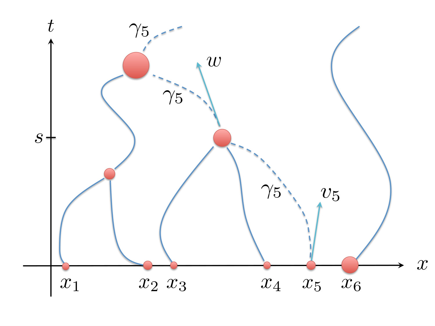 Figure 1
Peer Reviews
No public reviews on file for this paper yet. If you reviewed it on a platform where reviews are public (OpenReview, ICLR, NeurIPS, ICML), you can paste yours below so the community can read it here.
Videos
No videos yet. Explain this paper in a talk, walkthrough, or lecture? Add one.
A trajectory map for the pressureless Euler equations
Ryan Hynd
Abstract
We consider the dynamics of a collection of particles that interact pairwise and are restricted to move along the real line. Moreover, we focus on the situation in which particles undergo perfectly inelastic collisions when they collide. The equations of motion are a pair of partial differential equations for the particles’ mass distribution and local velocity. We show that solutions of this system exist for given initial conditions by rephrasing these equations in Lagrangian coordinates and then by solving for the associated trajectory map.
1 Introduction
In this paper, we will study the dynamics of a collection of particles which interact pairwise and which moves along the real line. We will also suppose that when particles collide, they undergo perfectly inelastic collisions. The equations of motion for this type of physical system are the pressureless Euler equations
[TABLE]
which hold on . The first equation expresses the conservation of mass, and the second expresses the conservation of momentum. Here and are the respective mass distribution and velocity field of particles and is the interaction energy.
The central goal of this work is to describe how to find a pair and which solves (1.1) for given initial conditions
[TABLE]
We typically will assume belongs to the space of Borel probability measures on and is continuous. To this end, we will first produce which satisfies the pressureless Euler flow equation
[TABLE]
and the initial condition
[TABLE]
almost everywhere. Here
[TABLE]
is the push forward of under , and is the conditional expectation of a Borel given .
To emphasize that is a function on , we will sometimes write
[TABLE]
The quantity represents the time position of a particle which was initially at position . After showing a solution exists, we will argue that there is a Borel function such that
[TABLE]
almost everywhere. In particular, we will see that
[TABLE]
and together comprise an appropriately defined weak solution pair for the pressureless Euler system.
1.1 Main theorem
Throughout this paper, we will assume the has finite second moment
[TABLE]
and
[TABLE]
We will also suppose is continuously differentiable, is even
[TABLE]
and grows at most linearly
[TABLE]
Moreover, we will suppose that is semiconvex. That is,
[TABLE]
for some . We recall that concave corresponds to repulsive interaction between particles. Assuming that is semiconvex forces for Lebesgue almost every , which in a sense limits repulsive interaction.
Theorem 1.1**.**
There is a locally Lipschitz continuous which satisfies the pressureless Euler flow equation (1.3) and the initial condition (1.4). Moreover, has the following properties.
- (i)
For Lebesgue almost every with
[TABLE]
where
[TABLE] 2. (ii)
For and with ,
[TABLE] 3. (iii)
For and ,
[TABLE]
A few remarks about the statement of this theorem are in order. Locally Lipschitz means that is Lipschitz continuous for each , and consequently,
[TABLE]
exists in for almost almost every . The function in condition represents the total energy of the physical system being modeled by the pressureless Euler flow equation. Condition asserts that is nondecreasing and absolutely continuous on the support of
[TABLE]
Property asserts that is quantitatively “sticky.” That is, it quantifies the fact that if , then for all .
We will show that the existence of a weak solution of (1.1) for given initial conditions is a corollary of Theorem 1.1. In particular, we will verify that defined in (1.5) and any Borel which satisfies (1.6) is a weak solution of the pressureless Euler system whose energy
[TABLE]
is essentially nonincreasing in and which satisfies the one sided Lipschitz condition
[TABLE]
for almost every .
1.2 Prior work
We have already established the existence of a weak solution pair to the pressureless Euler system with an even, continuously differentiable, semiconvex potential. In [15], we generated this solution via a Borel probability measure on the space of continuous paths endowed with the topology of local uniform convergence. Specifically, we constructed an which satisfies: for each bounded, continuous and almost every
[TABLE]
where is defined via
[TABLE]
there is a Borel , such that
[TABLE]
for almost every . Then we checked that and is indeed a weak solution pair.
Along the way, we derived some specific information on such as it is concentrated on absolutely continuous paths, it satisfies various energy estimates, and
[TABLE]
for and almost every . We consider Theorem 1.1 to be a refinement of the main result in [15] as it tells us that we can choose as the push forward of under the map . Here is the path , which is continuous for almost every . That is, can be specified as
[TABLE]
for each that is continuous and bounded.
There have been many other works on pressureless Euler type systems in one spatial dimension. Especially since they are special cases of the multidimensional systems of equations which arise in the study of galaxy formation [14, 24]. One of the early mathematical works on this topic was by E, Rykov and Sinai [9], where they studied the case which corresponds to gravitational interaction between a collection of interacting particles constrained to move along the real line. We acknowledge that the existence of solutions for this particular case does not follow from Theorem 1.1 as isn’t continuously differentiable. Nevertheless, we will revisit this particular case below.
Another very influential study on this topic was done by Brenier, Gangbo, Savaré and Westdickenberg [4]. In comparison to our work, they considered general interactions which could be attractive or repulsive. We also note that they recast the pressureless Euler equations in another coordinate system, and they were able to obtain precise information about solutions from the resulting differential inclusions. Other work with related approaches were done by Gangbo, Nguyen, and Tudorascu [12] and Nguyen and Tudorascu [22] on the Euler-Poisson system and by Brenier and Grenier [5], Natile and Savaré [21], and Cavalletti, Sedjro and Westdickenberg [6] for the sticky particle system ( in (1.1) or equation (1.19) below). We also recommend the additional references [2, 7, 13, 17, 18, 19, 20, 23] for results on stationary solutions, local existence, uniqueness, and hydrodynamic limits related to pressureless Euler type systems.
The particular approach we take in this paper is motivated by the work of Dermoune [8] on the sticky particle system
[TABLE]
In particular, Dermoune was the first to identify that
[TABLE]
is the natural equation for the sticky particle system in Lagrangian variables. We performed a thorough analysis of (1.20) in [16] and regard Theorem 1.1 as a significant generalization of the main results of [16].
1.3 Euler-Poisson equations
As mentioned above, we will also consider the Euler-Poisson equations
[TABLE]
Here
[TABLE]
and the associated interaction potential is . This system governs the dynamics of a collection of particles in which the force on each particle is proportional to the total mass to the right of the particle minus the total mass to the left of the particle; when particles collide, they undergo perfectly inelastic collisions [4, 9]. This is a simple model for gravitationally interacting particles which are constrained to move on the real line.
As we did for the pressureless Euler system, we will design a trajectory mapping which satisfies the Euler-Poisson flow equation
[TABLE]
and the initial condition (1.4). However, since sgn is not continuous, we will have to argue a bit differently than we did to prove Theorem 1.1 in order to obtain the following theorem.
Theorem 1.2**.**
There is a Lipschitz continuous which satisfies the Euler-Poisson flow equation (1.23) and the initial condition (1.4). Moreover, has the following properties.
- (i)
For Lebesgue almost every with
[TABLE]
where
[TABLE] 2. (ii)
For and with ,
[TABLE] 3. (iii)
For and ,
[TABLE]
As with the pressureless Euler system, we will be able to generate a weak solution pair of the Euler-Poisson system a the solution obtained in Theorem 1.2. Namely, defined in (1.5) and any Borel which satisfies (1.6) is a weak solution of the Euler-Poisson system whose total energy
[TABLE]
is nonincreasing in time and which fulfills the “entropy” inequality
[TABLE]
for almost every .
The organization of this paper is as follows. First, we will review a few preliminaries needed for our study in section 2. Then we will show by a near explicit construction how to solve the pressureless Euler flow equation when the support of is finite in section 3. In section 4, we will analyze these special solutions and show they are compact in a certain sense. This compactness will allow us to solve the pressureless Euler flow equation for a general and consequently to solve the pressureless Euler equations for given initial conditions. Finally, in section 5, we will show how to alter the arguments we used for the pressureless Euler flow equation to solve the flow equation associated with the Euler-Poisson equations.
2 Preliminaries
In this section, we will briefly recall the facts we will need regarding the convergence of probability measures and conditional expectation.
2.1 Convergence of probability measures
As in the introduction, we denote as the space of Borel probability measures on . We will also write for the space of bounded continuous functions on . We will say that a sequence converges to in narrowly provided
[TABLE]
for every . It turns out that converges to narrowly if and only if , where is a metric of the form
[TABLE]
Here each satisfies
[TABLE]
for (Remark 5.1.1 of [1]). Furthermore, is a complete metric space.
We will need to be able to identify when a sequence of measures in has a narrowly convergent subsequence. Fortunately, Prokhorov’s theorem provides a necessary and sufficient condition; it asserts that has a narrowly convergent subsequence if and only if there is with compact sublevel sets such that
[TABLE]
(Theorem 5.1.3 of [1]). In addition, we will need to know when (2.1) holds for unbounded . It turns out that if is continuous and
[TABLE]
uniformly in , then (2.1) holds (Lemma 5.1.7 of [1]). In this case, we say that is uniformly integrable with respect to the sequence .
The following lemma will also prove to be useful.
Lemma 2.1** (Lemma 2.1 of [16]).**
Suppose is a sequence of continuous functions on which converges locally uniformly to and converges narrowly to . Further assume there is with compact sublevel sets, which is uniformly integrable with respect to and satisfies
[TABLE]
for each . Then
[TABLE]
2.2 The push-forward
Suppose is Borel measurable and . We define the push-forward of through as the probability measure which satisfies
[TABLE]
for every . We note
[TABLE]
for Borel . Moreover, if is continuous and narrowly in , then
[TABLE]
in .
2.3 Conditional expectation
Suppose , and is a Borel measurable function. A conditional expectation of with respect to given is an function which satisfies two conditions:
[TABLE]
for each Borel with ; and
[TABLE]
almost everywhere for a Borel with . The existence and almost everywhere uniqueness of a conditional expectation can be proved using the Radon-Nikodym theorem.
We emphasize that satisfies the pressureless Euler flow equation (1.3), provided the following two conditions hold for almost every :
[TABLE]
for each ; and there exists a Borel for which
[TABLE]
almost everywhere.
3 Sticky particle trajectories
In this section, we will assume that is a convex combination of Dirac measures
[TABLE]
In particular, we suppose that are distinct and with . We also define
[TABLE]
for . It turns out that there is a natural ODE system related to the pressureless Euler flow equation, which is
[TABLE]
These are Newton’s equations for interacting particles with masses ; the positions of these particles are described by the trajectories .
It turns out that a solution of the pressureless Euler flow equation can be built from these particle trajectories by first setting
[TABLE]
However, when trajectories intersect, we must modify the paths. Remarkably, the natural thing to do is to require that the corresponding particles undergo perfectly inelastic collisions when they collide. This amounts to requiring that the trajectories coincide and that their slopes average from the moment they intersect. On any time interval when no collisions occur, the resulting trajectories will satisfy (3.2). We will call these paths sticky particle trajectories and we shall see that they are the building blocks for more general solutions.
The following proposition asserts that these trajectories exist and satisfy a few basic properties.
Proposition 3.1** (Proposition 2.1 [15]).**
There are continuous, piecewise paths
[TABLE]
*with the following properties.
(i) For and all but finitely many , (3.2) holds.
(ii) For ,*
[TABLE]
(iii) For , and imply
[TABLE]
(iv) If , , and
[TABLE]
for , then
[TABLE]
for .
Remark 3.2*.*
Using property , it is routine to check that both exist for each and . Moreover,
[TABLE]
A corollary of property above is the what we call the averaging property. It is a general assertion about the conservation of momentum and is stated as follows.
Corollary 3.3** (Proposition 2.6 of [15]).**
Suppose and . Then
[TABLE]
3.1 Quantitative stickiness
Recall our standing assumption that there is a constant chosen so that is convex. In terms of this constant, we can quantify in Proposition 3.1. Namely, we can estimate the distance in terms of the distance for . This is why we call the following assertion the quantitative sticky particle property.
Proposition 3.4** (Proposition 2.5 of [15]).**
For each and
[TABLE]
An immediate corollary is as follows.
Proposition 3.5**.**
For each , there is a function for which
[TABLE]
for and
[TABLE]
for
Proof.
By property of Proposition 3.1, the cardinality of the set
[TABLE]
is nonincreasing in . It follows that there is a surjective function
[TABLE]
for . By the quantitative sticky particle property, satisfies the Lipschitz condition (3.5). We can then extend to all of in order to obtain the desired Lipschitz function . ∎
3.2 Energy estimates
Sticky particle trajectories have nonincreasing energy. That is,
[TABLE]
for (Proposition 2.8 of [15]). Using the semiconvexity of , we can derive the subsequent kinetic energy estimates. We will express this result in terms of the increasing function
[TABLE]
Lemma 3.6**.**
For each ,
[TABLE]
And for all but finitely many ,
[TABLE]
Proof.
Due to the convexity of ,
[TABLE]
Combining these lower bounds with (3.6) at gives
[TABLE]
for all but finitely many . As a result,
[TABLE]
for all but finitely many . We can then integrate from [math] to to derive (3.7). Inequality (3.8) follows from (3.7) and (3.9). ∎
3.3 Stability estimate
We need one more estimate that depends on the following elementary lemma.
Lemma 3.7**.**
Suppose and is continuous and piecewise . Further assume
[TABLE]
for each and that there is for which
[TABLE]
for all but finitely many . Then
[TABLE]
for .
Proof.
By a routine scaling argument, it suffices to verify this assertion for . To this end, we suppose in addition that there are times for which is on the intervals .
Define
[TABLE]
so that Observe
[TABLE]
and
[TABLE]
for . Consequently,
[TABLE]
for .
In view of (3.13),
[TABLE]
for Multiplying through by and integrating from [math] to gives
[TABLE]
That is,
[TABLE]
for .
By (3.10) and (3.13), we likewise have
[TABLE]
for . Again we multiply through by and integrate from to to get
[TABLE]
In particular, (3.15) holds for . We can argue similarly to show that (3.15) also holds on the intervals . ∎
This leads to a stability estimate.
Proposition 3.8**.**
Suppose , and . Then
[TABLE]
Proof.
Without loss of generality, we may assume so that the sticky particle trajectories are ordered . Under this assumption, it suffices to verify
[TABLE]
for . For if with ,
[TABLE]
To this end, we fix and set
[TABLE]
In order to verify (3.17), it is enough to show
[TABLE]
We will do so by applying the previous lemma to the restriction of the function
[TABLE]
to . In particular, we note that for whenever is finite.
We first claim
[TABLE]
Note that if does not have a first intersection time at , then is near and so
[TABLE]
Alternatively let us suppose has a first intersection time at . As a result, there are trajectories such that
[TABLE]
and
[TABLE]
.
Also note that as for ,
[TABLE]
for all small. By Remark 3.2, we can send and conclude
[TABLE]
It then follows from (3.25) (with ) that
[TABLE]
which is (3.24). A similar argument gives
[TABLE]
for each . Combining (3.24) and (3.26)
[TABLE]
for all .
As is nondecreasing,
[TABLE]
for all but finitely many . Therefore, (3.23) follows from Lemma 3.7. ∎
3.4 Associated trajectory map
We are now ready to show how to design a solution of (1.3) with given by (3.1). For , we define
[TABLE]
We will also write
[TABLE]
for and . The following proposition details all the important features of .
Proposition 3.9**.**
The mapping has the following properties.
- (i)
* and*
[TABLE]
for all but finitely many . Both equalities hold on the support of . 2. (ii)
, for . Here
[TABLE] 3. (iii)
* is locally Lipschitz continuous.* 4. (iv)
For and with ,
[TABLE] 5. (v)
For each and
[TABLE] 6. (vi)
For each , there is a function which satisfies the Lipschitz condition (3.5) and
[TABLE]
for .
Proof.
Part : As ,
[TABLE]
on . Also note that if and , then Corollary 3.3 gives
[TABLE]
In particular,
[TABLE]
for all but finitely many .
Define
[TABLE]
By parts and of Proposition 3.1, is well defined. Moreover, it is routine to check that is Borel measurable. Furthermore,
[TABLE]
on the support of for all but finitely many . It follows that satisfies the pressureless Euler flow equation (1.3) for all but finitely many .
Part : In view of (3.6),
[TABLE]
Part : By the energy estimate (3.8),
[TABLE]
Since is smooth, is locally Lipschitz continuous.
Part , Part and : Part follows from Proposition 3.8, Part is a corollary of Proposition 3.4, and part is due to Corollary 3.5. ∎
Observe that as is absolutely continuous,
[TABLE]
tends to [math] as and is sublinear. By part of the above proposition,
[TABLE]
for belonging to the support of . As a result, is uniformly continuous on the support of . In particular, we may extend to a uniformly continuous function on which satisfies (3.35) and agrees with on the support of . Without any loss of generality, we will identify with this extension and assume is uniformly continuous on .
4 Existence of solutions
Now let with
[TABLE]
We can select a sequence such that each is a convex combination of Dirac measures, narrowly, and
[TABLE]
We recommend, for instance, the reference [3] for a discussion on how to design such a sequence.
In view of Proposition 3.9, there is a locally Lipschitz continuous mapping which satisfies
[TABLE]
for each . Here
[TABLE]
In this section, we will show that there is a subsequence of which converges in an appropriate sense to a solution of the pressureless Euler flow equation (1.3) and satisfies (1.4). Then we will show how to use this solution to generate a corresponding weak solution of the pressureless Euler equations.
4.1 Compactness
We will prove that has a subsequence which converges in a strong sense. The limit mapping will be our candidate for a solution of the pressureless Euler flow equation.
Proposition 4.1**.**
There is a subsequence and a locally Lipschitz such that
[TABLE]
for each and continuous with
[TABLE]
Furthermore, has the following properties.
- (i)
For and with ,
[TABLE] 2. (ii)
For each and
[TABLE] 3. (iii)
For each , there is a function which satisfies the Lipschitz condition (3.5) and
[TABLE]
for .
Proof.
- Weak convergence: Define
[TABLE]
for and . By (3.30),
[TABLE]
And as and grow at most linearly, there are constants
[TABLE]
for each and .
It follows that
[TABLE]
for each As a result, is narrowly precompact. Moreover, for Lipschitz continuous ,
[TABLE]
In terms of the metric (2.2), we then have
[TABLE]
for and .
By the Arzelà-Ascoli, there is a subsequence and a narrowly continuous path such that uniformly for belonging to compact subsets of . We can also use this narrow convergence and (4.7) to show
[TABLE]
for each . Further,
[TABLE]
for .
By the disintegration theorem (Theorem 5.3.1 of [1]), there is a family of probability measures for which
[TABLE]
Set
[TABLE]
and as before we will write . Observe
[TABLE]
for each .
- Strong convergence: By (3.35),
[TABLE]
for . As , is uniformly equicontinuous. Moreover,
[TABLE]
and integrating over gives
[TABLE]
By (4.2) and the at most sublinear growth of , there are constants such that
[TABLE]
for , and .
It follows that a subsequence of (which we will not relabel) converges locally uniformly on to a continuous function . It is easy to check
[TABLE]
for each . So if has another subsequence which converges locally uniformly on to , then
[TABLE]
In particular, almost everywhere. Since and are continuous, it is routine to check that on the entire support of .
By (4.1), we also have that almost everywhere. Without loss of generality, we can redefine to ensure that locally uniformly on . By estimate (4.15) and Proposition 2.1, we also have
[TABLE]
In particular,
[TABLE]
which when combined the narrow converge in gives (4.4).
In view of (3.30), we also have
[TABLE]
Here we used that and are continuous and grow at most linearly. Therefore, the mapping is locally Lipschitz continuous.
- Properties of the limit: Suppose with . As narrowly in , there are sequences such that and (Proposition 5.1.8 in [1]). Without any loss of generality, we may suppose that for all as this occurs for all large enough. By part of Proposition 3.9,
[TABLE]
Since locally uniformly, we can send in order to conclude property of this theorem. Property can be proved similarly.
Now let and . As above, we may select such that . Appealing to part of Proposition 3.9, there is a sequence of functions in which each element satisfies the Lipschitz condition (3.5) and
[TABLE]
for each . In particular,
[TABLE]
As and locally uniformly, is bounded above for belonging to compact subsets of independently of . As a result, has a locally uniformly convergent subsequence. Therefore, we can send along an appropriate subsequence in (4.21) to obtain part . ∎
For the remainder of this section, let denote the mapping obtained in Proposition 4.1.
Corollary 4.2**.**
For Lebesgue almost every , there is a Borel function for which
[TABLE]
* almost everywhere.*
Proof.
Let be a time such that
[TABLE]
in . We recall that since is locally Lipschitz, the set of all such has full measure in . Moreover, we may suppose that the limit (4.23) holds almost everywhere in as it does for a subsequence. By Theorem 1.19 in [11], we may further assume that the limit (4.23) holds everywhere on some Borel with .
In view of part of Proposition 4.1,
[TABLE]
on . Here
[TABLE]
is a Borel measurable function for each . Consequently, is measurable with respect to the Borel sigma-sub-algebra generated by
[TABLE]
As is a pointwise limit of measurable functions, it is measurable itself (Proposition 2.7 [11]). It follows that there is a Borel function such that
[TABLE]
That is, almost everywhere. ∎
Proof of Theorem 1.1.
-
Initial condition: The limit (4.4) taken when implies almost everywhere.
-
Flow equation: We next claim
[TABLE]
for each continuous which satisfies
[TABLE]
and each . In view of Corollary 4.2, this would imply that is a solution of the pressureless Euler flow equation. To this end, we set for and note that grows at most quadratically. By Proposition 4.1,
[TABLE]
Consequently,
[TABLE]
Let us fix for the moment and consider the integral
[TABLE]
In view of Proposition 4.1 and the at most linear growth of ,
[TABLE]
as . Also observe
[TABLE]
locally uniformly for and each fixed .
Choosing so large that
[TABLE]
gives
[TABLE]
for and . Here are the constants from inequality (4.15).
We can then appeal to Proposition 2.1 to conclude
[TABLE]
for each . What’s more, (4.1) implies
[TABLE]
for . The limit (4.2) and a standard variant of dominated convergence (Theorem 1.20 in [10]) together give
[TABLE]
As a result,
[TABLE]
Since
[TABLE]
and the integrals are bounded and converge for each as , we likewise have
[TABLE]
The claim (4.24) then follows by sending in
[TABLE]
- Properties of the solution: Assertions and of this claim follow from parts and of Proposition 4.1, respectively. So we will now focus on verifying assertion which states that
[TABLE]
is essentially nonincreasing on . Recall that
[TABLE]
is nonincreasing by part of Proposition 4.1.
As solves the pressureless Euler flow equation, we can integrate by parts to find
[TABLE]
The limit (4.30) with and and the limit (4.35) with give
[TABLE]
for each .
Next, we claim that
[TABLE]
for each . Note that grows at most quadratically. Indeed,
[TABLE]
for as is semiconvex. Likewise
[TABLE]
and so
[TABLE]
Since grows at most linearly, it must be that
[TABLE]
for some constant .
Combining (4.47) and (4.15), it is routine to check
[TABLE]
for each , , . Note that
[TABLE]
locally uniformly for for each . Also observe that narrowly in , and
[TABLE]
which implies that is uniformly integrable with respect to . It follows from Lemma 2.1 that (4.43) holds for each .
In view of estimate (4.48), we can also apply a standard variant of dominated convergence to find
[TABLE]
for each . Combining with (4.40) gives
[TABLE]
for each . As is uniformly bounded and nonincreasing, also converges for each by Helly’s selection theorem (Lemma 3.3.3 in [1]). By (4.53), for almost every . We then conclude that for almost every with
[TABLE]
∎
4.2 Solution of the pressureless Euler equations
We are now in position to establish the existence of a weak solution of the pressureless Euler equations (1.1) which satisfy the initial conditions (1.2). These types of solutions are defined as follows.
Definition 4.3**.**
A narrowly continuous and a Borel measurable is a weak solution pair of the pressureless Euler equations (1.1) which satisfies the initial conditions (1.2) if the following hold.
For each ,
[TABLE]
For each ,
[TABLE]
For each ,
[TABLE]
Corollary 4.4**.**
There exists a weak solution pair and of the pressureless Euler equations (1.1) which satisfies the initial conditions (1.2). Moreover, this solution pair has the following two properties.
- (i)
For almost every ,
[TABLE] 2. (ii)
For almost every and almost every ,
[TABLE]
Proof.
- Specifying : Let denote the solution of the pressureless Euler flow equation (1.3) which satisfies (1.4) as described in Theorem 1.1 and define
[TABLE]
for Borel . This clearly defines a signed Borel measure on , and it is not hard to check that is sigma finite. Let us also set
[TABLE]
for Borel . It is clear that it is also sigma finite and that is absolutely continuous with respect to .
By the Radon-Nikodym theorem, there is a Borel measurable such that
[TABLE]
Note in particular that
[TABLE]
for each continuous with compact support. It follows that
[TABLE]
almost everywhere.
- Integrability: Since is locally Lipschitz,
[TABLE]
for each . Lipschitz continuity also implies that is bounded on , so
[TABLE]
Thus, and satisfy part of Definition 4.3.
- Weak solution property: Suppose
[TABLE]
This proves part of Definition 4.3. As for part that definition,
[TABLE]
- Nonincreasing energy and entropy inequality: Since
[TABLE]
for almost every , for almost every with . Here, of course, we are employing conclusion of Theorem 1.1.
Recall that is absolutely continuous on any compact interval within for almost every . Let us denote this set of as , and we emphasize that is measurable and . By conclusion of Theorem 1.1,
[TABLE]
for Lebesgue almost every and .
As a result, we have proved part of this assertion for belonging to the image of under
[TABLE]
for almost every . Without loss of generality, we may suppose is a countable union of closed sets (Theorem 1.19 of [11]). By part of Theorem 1.1, we may as well assume is continuous on . It follows that is Borel measurable (Proposition A.1 in [16]). As ,
[TABLE]
We conclude that part of this assertion holds for Lebesgue almost every and belonging to a Borel set of full measure for . ∎
5 Euler-Poisson equations in 1D
For the remainder of this paper, we will assume
[TABLE]
As is not continuously differentiable, we will also consider the closely related interaction potential
[TABLE]
for and small. Clearly,
[TABLE]
Also observe that is convex, even, and continuously differentiable with
[TABLE]
Therefore, there is a locally Lipschitz continuous which satisfies
[TABLE]
for each . Here
[TABLE]
We will argue below that there is a sequence of positive numbers and which converges in a strong sense to a solution of the Euler-Poisson flow equation (1.23) which satisfies the initial condition (1.4). We will then make a final remark on the existence of weak solution pairs to the Euler-Poisson system (1.21).
5.1 A strongly convergent subsequence
Let us begin by recalling a few facts we have already established for .
Lipschitz continuity in time. In view of Theorem 1.1, satisfies
[TABLE]
for almost every . Therefore, is uniformly Lipschitz continuous.
Uniform spatial continuity. Theorem 1.1 also gives
[TABLE]
for each with and for each . As a result, we may was well suppose is uniformly continuous and satisfies
[TABLE]
for every and . Here is the modulus of continuity defined in (3.34).
Quantitative stickiness. For , there is a function which satisfies
[TABLE]
such that
[TABLE]
for . In particular,
[TABLE]
for and .
We can use this Lipschitz continuity in time, uniform spatial continuity and quantitative stickiness of , along with the arguments we used to prove Proposition 4.1 and Corollary 4.2, to establish the following assertion.
Proposition 5.1**.**
There is a sequence of positive numbers and a Lipschitz such that for each ,
[TABLE]
locally uniformly on and
[TABLE]
for continuous with
[TABLE]
In addition, has the following properties.
- (i)
For and with ,
[TABLE] 2. (ii)
For each and
[TABLE] 3. (iii)
For each , has a subsequence which converges locally uniformly to a function which satisfies the Lipschitz condition (5.12) and
[TABLE]
for . 4. (iv)
For almost every , there is a Borel function for which
[TABLE]
for almost everywhere.
We also have the following immediate corollary which can be proved the same way that we justified (4.26).
Corollary 5.2**.**
Suppose is continuous and
[TABLE]
Then
[TABLE]
for .
This is as far as we can go with the convergence arguments we used to establish Theorem 1.1. We will need to identify another mechanism which will allow us to pass to the limit in the term with in equation (5.5). This will be the topic of the following subsection.
5.2 A convergence lemma
Let us recall the definition of sgn
[TABLE]
We will also fix a sequence which converges narrowly to and additionally satisfies
[TABLE]
The central assertion of this subsection is as follows.
Lemma 5.3**.**
Suppose is continuous and
[TABLE]
Then
[TABLE]
We will first verify an elementary observation, which is ultimately due to the convexity of the absolute value function. In particular, we will employ
[TABLE]
for each .
Lemma 5.4**.**
*The following are equivalent for .
(i) For almost every ,*
[TABLE]
(ii) For each continuous which satisfies (5.23),
[TABLE]
Proof.
Suppose is a continuous function which grows at most linearly as .
Employing (5.25) and noting that sgn is odd gives
[TABLE]
By assumption,
[TABLE]
Also notice
[TABLE]
and
[TABLE]
for . By dominated convergence, we can send in (5.26) to find
[TABLE]
Replacing with gives
[TABLE]
As is arbitrary, vanishes almost everywhere. ∎
Proof of Lemma 5.5.
Using the same method to prove in Lemma 5.4, we find
[TABLE]
for each continuous and at most linearly growing . And by (5.3),
[TABLE]
Since ,
[TABLE]
Combining this fact with (5.22) provides a subsequence and such that
[TABLE]
for each continuous and at most linearly growing (Theorem 5.4.4 of [1]). Sending in (5.27) gives
[TABLE]
Lemma 5.4 implies
[TABLE]
Since this limit is independent of the subsequence,
[TABLE]
for each continuous which satisfies (5.5). ∎
We will actually need a minor refinement of Lemma 5.4 in our proof of Theorem 1.2.
Corollary 5.5**.**
Suppose is a sequence of continuous functions on which satisfies
[TABLE]
for some and which converges locally uniformly to . Then
[TABLE]
Proof.
As for each , we also have
[TABLE]
Fix and choose a compact interval such that
[TABLE]
for ; such an interval exists as is uniformly integrable with respect to by assumption (5.22). In view of Lemma 5.4,
[TABLE]
as .
Observe
[TABLE]
And by (5.31),
[TABLE]
As a result,
[TABLE]
The claim follows as was arbitrarily chosen. ∎
5.3 Solution of the flow equation
This subsection is dedicated to the proof of Theorem 1.2. Here, we will show that the mapping obtained in Proposition 5.1 is a solution flow equation (1.23) which has all of the required properties. First note that since and in as , then . Next we claim that satisfies flow equation (1.23). It suffices to let , fix a continuous which satisfies
[TABLE]
and show
[TABLE]
Once we establish this identity, parts , and of Theorem 1.2 would follow by minor variations of the arguments we gave in our proof of Theorem 1.1.
To this end, we recall that for each ,
[TABLE]
Moreover, Proposition 5.1 implies
[TABLE]
narrowly and
[TABLE]
for each .
Proposition 5.1 also can be used to show
[TABLE]
Furthermore,
[TABLE]
as noted in Corollary 5.2. As a result, we are left to justify the limit
[TABLE]
Then we would be able to send in (5.33) to conclude (5.32).
So we will now focus on establishing (5.38). Observe
[TABLE]
Since is uniformly bounded and grows at most linearly, we just need to show
[TABLE]
for each with . For if (5.42) holds, (5.38) would follow from a simple application of the dominated convergence theorem.
In view of (5.13),
[TABLE]
By part of Proposition 5.1, locally uniformly on (up to a subsequence that we will not relabel) and
[TABLE]
almost everywhere. It follows that converges locally uniformly to . We also have the limits (5.34) and (5.35) for each . We can then apply Corollary 5.5 once we know grows at most linearly in in a uniform way.
Fix and observe
[TABLE]
for all . Since as , it must be that
[TABLE]
Corollary 5.5 then gives
[TABLE]
We conclude (5.42) and in turn that is a solution of the flow equation (1.23).
5.4 Solving the Euler-Poisson equations
Weak solution pairs of the Euler-Poisson system (1.21) which satisfy given initial conditions (1.2) are defined as follows.
Definition 5.6**.**
A narrowly continuous and a Borel measurable is a weak solution pair of the Euler-Poisson equations (1.21) which satisfies the initial conditions (1.2) if the following hold.
For each ,
[TABLE]
For each ,
[TABLE]
For each ,
[TABLE]
Employing the same method used to prove Corollary 4.4 from Theorem 1.1, we have the subsequent corollary to Theorem 1.2.
Corollary 5.7**.**
There exists a weak solution pair and of the Euler-Poisson equations (1.21) which satisfies the initial conditions (1.2). Moreover, this solution pair additionally has the following features.
- (i)
For almost every with ,
[TABLE] 2. (ii)
For almost every and almost every ,
[TABLE]
The reference list from the paper itself. Each links out to its DOI / PubMed record.
- 1[1] L. Ambrosio, N. Gigli, and G. Savaré. Gradient flows in metric spaces and in the space of probability measures . Lectures in Mathematics ETH Zürich. Birkhäuser Verlag, Basel, second edition, 2008.
- 2[2] M. Bézard. Existence locale de solutions pour les équations d’Euler-Poisson. Japan J. Indust. Appl. Math. , 10(3):431–450, 1993.
- 3[3] F. Bolley. Separability and completeness for the Wasserstein distance. In Séminaire de probabilités XLI , volume 1934 of Lecture Notes in Math. , pages 371–377. Springer, Berlin, 2008.
- 4[4] Y. Brenier, W. Gangbo, G. Savaré, and M. Westdickenberg. Sticky particle dynamics with interactions. J. Math. Pures Appl. (9) , 99(5):577–617, 2013.
- 5[5] Y. Brenier and E. Grenier. Sticky particles and scalar conservation laws. SIAM J. Numer. Anal. , 35(6):2317–2328, 1998.
- 6[6] F. Cavalletti, M. Sedjro, and M. Westdickenberg. A simple proof of global existence for the 1D pressureless gas dynamics equations. SIAM J. Math. Anal. , 47(1):66–79, 2015.
- 7[7] Y. Deng, T.-P. Liu, T Yang, and Z. Yao. Solutions of Euler-Poisson equations for gaseous stars. Arch. Ration. Mech. Anal. , 164(3):261–285, 2002.
- 8[8] A. Dermoune. Probabilistic interpretation of sticky particle model. Ann. Probab. , 27(3):1357–1367, 1999.