TL;DR
This paper develops methods for tuning edge weights in fixed-topology networks to satisfy controllability metrics, using convex relaxations and optimization, with applications demonstrated on power systems.
Contribution
It introduces a convex relaxation approach for controllability-based edge weight tuning and proposes a sparsity-promoting cost function for network design.
Findings
Convex relaxations effectively solve controllability feasibility problems.
Sparsity-promoting costs reduce the number of modified edges.
Numerical simulations validate the proposed methods on power system models.
Abstract
In this paper, we consider the problem of tuning the edge weights of a networked system described by linear time-invariant dynamics. We assume that the topology of the underlying network is fixed and that the set of feasible edge weights is a given polytope. In this setting, we first consider a feasibility problem consisting of tuning the edge weights such that certain controllability properties are satisfied. The particular controllability properties under consideration are (i) a lower bound on the smallest eigenvalue of the controllability Gramian, which is related to the worst-case energy needed to control the system, and (ii) an upper bound on the trace of the Gramian inverse, which is related to the average control energy. In both cases, the edge-tuning problem can be stated as a feasibility problem involving bilinear matrix equalities, which we approach using a sequence of convex…
Click any figure to enlarge with its caption.
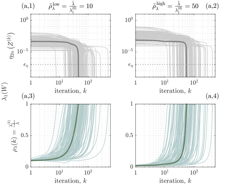 Figure 1
 Figure 2
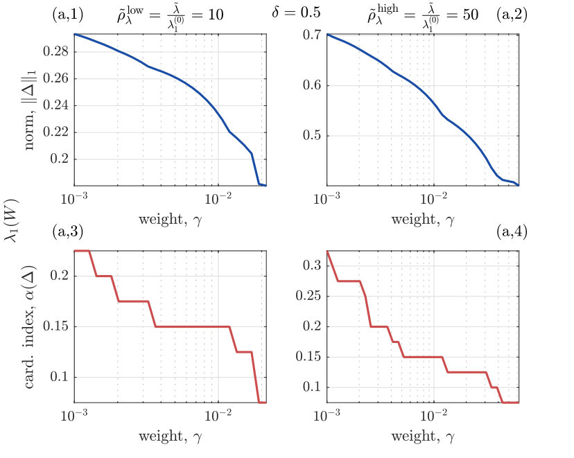 Figure 3
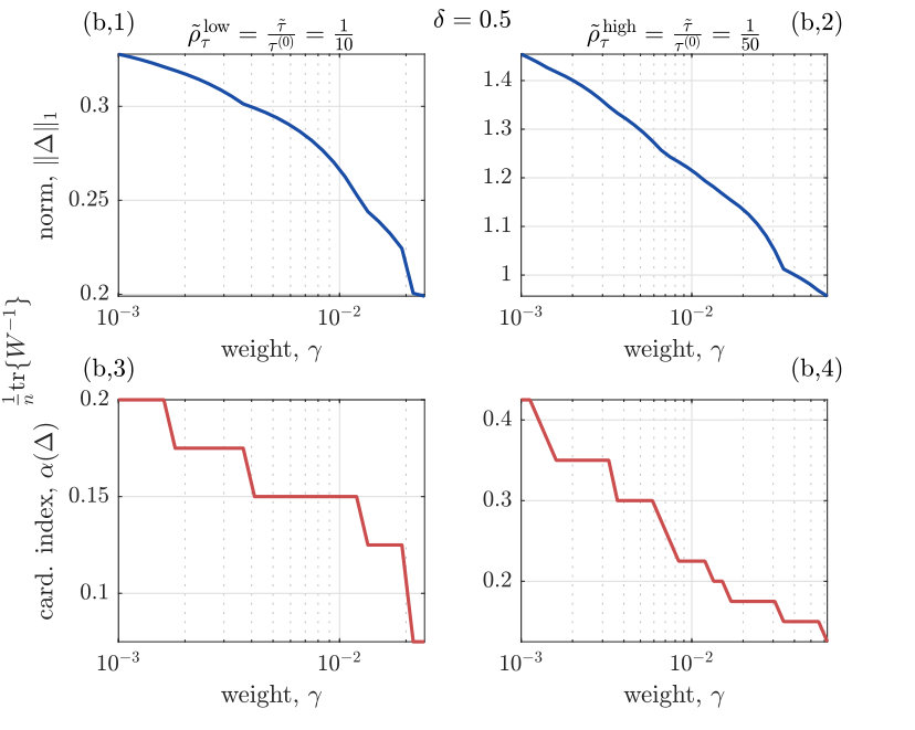 Figure 4
 Figure 5
Peer Reviews
No public reviews on file for this paper yet. If you reviewed it on a platform where reviews are public (OpenReview, ICLR, NeurIPS, ICML), you can paste yours below so the community can read it here.
Code & Models
Videos
No videos yet. Explain this paper in a talk, walkthrough, or lecture? Add one.
\DTLsetseparator
=
Network Design for Controllability Metrics
Cassiano O. Becker, Sérgio Pequito, George J. Pappas and Victor M. Preciado
This work was supported in part by the National Science Foundation, grant CAREER-ECCS-1651433 and in part by CAPES, Coordenação de Aperfeiçoamento de Pessoal de Nível Superior - Brasil.
Cassiano O. Becker ([email protected]), George J. Pappas ([email protected]) and Victor M. Preciado ([email protected]) are with the Department of Electrical and Systems Engineering, University of Pennsylvania - 200 South 33rd Street, Philadelphia, PA 19104. Sérgio Pequito ([email protected]) is with the Department of Industrial and Systems Engineering, Rensselaer Polytechnic Institute - CII 5007, 110 8th Street, Troy, NY 12180-3590.
Abstract
In this paper, we consider the problem of tuning the edge weights of a networked system described by linear time-invariant dynamics. We assume that the topology of the underlying network is fixed and that the set of feasible edge weights is a given polytope. In this setting, we first consider a feasibility problem consisting of tuning the edge weights such that certain controllability properties are satisfied. The particular controllability properties under consideration are (i) a lower bound on the smallest eigenvalue of the controllability Gramian, and (ii) an upper bound on the trace of the Gramian inverse. In both cases, the edge-tuning problem can be stated as a feasibility problem involving bilinear matrix equalities, which we approach using a sequence of convex relaxations. Furthermore, we also address a design problem consisting of finding edge weights able to satisfy the aforementioned controllability constraints while seeking to minimize a cost function of the edge weights, which we assume to be convex. Finally, we verify our results with numerical simulations over many random network realizations, as well as with an IEEE 14-bus power system topology.
Index Terms:
Networked dynamics, network design, controllability Gramian, bilinear matrix equality, convex optimization.
I Introduction
Many technological, biological, chemical, and social systems can be modeled as large ensembles of dynamical units connected via an intricate pattern of interactions [1]. From an engineering perspective, we are interested in efficiently steering the dynamics of these complex systems via external actuation. In this direction, control theory provides us with the notion of controllability to decide whether a given system can be steered towards an arbitrary state [2]. Furthermore, the so-called controllability Gramian of a system, which implicitly depends on the system’s dynamics and the configuration of its actuators, can be used to quantify the energy required to steer the system, assuming the system is controllable [2]. Leveraging these notions, several papers have recently focused on the problem of optimally allocating actuators throughout the network under several performance metrics [3, 4, 5, 6, 7, 8, 9, 10, 11, 12].
In some scenarios, instead of designing the location of external actuators, one may consider the alternative problem of modifying the network’s dynamics given a fixed configuration of actuators. For example, in power systems, one can tune the electrical parameters of the transmission lines using, for example, flexible AC transmission system (FACTS) devices [13, 14]. Also, in multi-agents networks, the interactions between agents can usually be modified to achieve a particular objective [15]. For instance, in leader-follower multi-agent networks, one may consider the scenario where both the communication topology and the location of the external actuators are fixed. Then, one can seek a set of edge weights (e.g., the agents’ update rules) such that the average and/or worst-case energy required to drive the state of the network satisfies certain bounds. In this regard, the present work first considers the feasibility problem of finding the edge weights of a linear networked system such that certain bounds on controllability metrics are satisfied. Secondly, we address the design problem of finding edge weights able to satisfy the aforementioned bounds while seeking to minimize a cost function of the edge weights, which we assume to be convex. In particular, we consider a -norm sparsity-promoting cost function aiming to penalize the number of edges whose weights are modified in the resulting design.
I-1 Related Work
In recent years, the problem of designing systems to satisfy certain controllability metrics has mostly focused on finding optimal actuator configurations, i.e., the location of those nodes to be externally actuated by control inputs [3, 4, 5, 6, 7, 8, 9, 10, 11, 12]. In addition, a considerable amount of research has been dedicated to understanding how the network topology impacts control performance [16, 17, 18, 19, 20, 21, 22, 23, 7, 24, 25]. In particular, [25] establishes necessary and sufficient graph-theoretical conditions for a discrete-time networked system to exhibit a diagonal controllability Gramian. In [26], the authors characterize the minimum input energy required to transfer a discrete-time dynamical system with bilinear dynamics from the origin to a desired state. The work in [27] proposes the notion of observability radius, which measures how much the parameters of a dynamical system can be perturbed before the system becomes unobservable. In a similar direction, the work in [28] investigates the effect of adding network edges to improve spectral performance metrics for the case of consensus dynamics over networks.
More generally, the works in [29, 30, 31, 32, 33] investigate design problems that seek to optimize network dynamical properties such as the dominant eigenvalue of the system matrix, with applications to virus spread and wireless control networks appearing in [34, 35, 36, 37].
The present paper extends previous work by the authors in [38] through several contributions. Specifically, in this paper we: (i) address the discrete-time case, in which the discrete Lyapunov equation introduces higher-degree products in its decision variables and requires new transformation steps for its treatment; (ii) provide an analysis of the conditions under which stability of the designed system is assured; (iii) consider cost functions over edge weights, which can be used to promote solutions with higher sparsity in edge modifications; (iv) propose a convex relaxation approach, which enables a more detailed analysis of convergence; (v) consider average controllability as an additional controllability metric; and (vi) present comprehensive computational experiments to illustrate the above aspects.
I-2 Structure and contributions of the paper
The rest of the paper is organized as follows. In Section II, we formalize both the network feasibility and the network design problems, in which we are tasked with tuning the weights of the edges in a given network in order to satisfy certain controllability metrics. Specifically, we consider two metrics: (i) the worst-case control energy, which is related to the smallest eigenvalue of the Gramian, and (ii) the average energy required to drive the system, which is related to the trace of the Gramian inverse. In Section III, we provide a detailed description of the strategy followed to solve both problems. In particular, we cast both the feasibility and the design problems into nonlinear optimization programs with quadratic bilinear terms, which are, in general, computationally hard to solve. We approach these optimization problems by lifting the space of variables and adding a rank constraint on a matrix whose entries depend affinely on the decision variables. We then propose a sequence of convex problems to relax this rank constraint using a truncated nuclear norm. In Section IV, we illustrate the validity of our results via computational experiments on random graphs, as well as a -norm sparsity-promoting design problem considering the IEEE 14-bus system. We conclude and enumerate some possibilities for future work in Section V.
Notation
We denote by the entry at the -th row and -th column of the matrix . The transpose of X is written as . The identity matrix is denoted by . The operator returns a diagonal matrix having as entries in its diagonal. The inner product between two matrices is given by ,
where denotes the trace operator.
The -norm of a matrix is defined as the -norm of its vectorization, i.e., .
Likewise, the [math]-norm of a matrix is defined as the -quasi-norm of its vectorization, i.e., the number of nonzero entries. The infinity norm of is defined as .
The nuclear norm of is defined in terms of its singular values , , as .
The operator norm of is denoted by and computed as , the largest singular value of .
We denote by the set of symmetric matrices of dimension . Likewise, (resp., ) is the set of symmetric positive semidefinite (resp., definite) matrices. Correspondingly, the semidefinite partial ordering is denoted (resp., ) when (resp., ).
A set is a spectrahedron [39, Def. 2.6] if it can be represented in the form , for .
A proper algebraic variety is the set of common zeros of a finite number of nonzero polynomials in variables.
II Problem Formulation
Consider a networked system following a discrete-time linear time-invariant dynamics, described by
[TABLE]
where denotes the vector of states and is the vector of inputs at instant . The sparsity pattern of the state matrix is constrained by a directed interdependency graph defined by a set of nodes and a set of edges , such that if the edge , and if . Also, the input matrix is such that if the external input signal directly influences , and otherwise.
Next, consider the problem of driving the state of the network from a given initial state to a desired target state within a time horizon , by designing a sequence of inputs for . If any is attainable from within a time horizon , then the system (1) is said to be reachable, which we refer to being reachable. Furthermore, it is known that the minimum input control energy to steer the system to a desired final state from is given by [2]
[TABLE]
where is called the finite-horizon reachability Gramian, defined as The infinite-horizon reachability Gramian is then obtained as the limit . This Gramian is positive definite, and can be computed as the (unique) solution to the discrete-time Lyapunov equation
[TABLE]
when the system is reachable and is stable [2].
II-A Reachability Metrics
We focus on two metrics related to the reachability Gramian to quantify the minimum input energy to drive the system [40, 16, 26].
Worst-case minimum input energy
Because is (symmetric) positive definite when the system is reachable, its eigenvalues are positive real numbers, with corresponding eigenvectors for . It turns out that the final state satisfying requiring the largest minimum input energy to be reached from is given by the (normalized) eigenvector . The energy required to drive the state from the origin towards within an infinite horizon is equal to , which we call the worst-case minimum input energy. Therefore, if we require the worst-case minimum input energy to be less than or equal to a desired value , then the reachability Gramian must satisfy the following semidefinite constraint:
[TABLE]
Average minimum input energy
The expected energy required to steer the system from the origin towards a random final state uniformly distributed over the unit sphere is equal to [40], which we call the average minimum input energy. In a manner similar to the worst-case minimum input energy metric, we can constrain the average minimum input energy to be upper-bounded by a target value via the condition
[TABLE]
which is also representable by a semidefinite constraint over (see Lemma A.3 in the Appendix).
In what follows, we will refer to the aforementioned reachability constraints on by the set membership condition
[TABLE]
where is a convex set (more precisely, a spectrahedron) defined by constraints (4) and/or (5), and indexed by the parameters in .
II-B Network Design for Reachability
As previously mentioned, we consider the problem of tuning the edge weights of a given network in order to satisfy certain minimum control energy requirements (either in worst-case or in average). In particular, we assume that we are able to add a matrix to the state matrix , such that presents the same sparsity pattern as the interdependency graph, i.e., for . After this addition, the dynamics of the network becomes
[TABLE]
Furthermore, we may require that be contained in a given polytope encoding acceptable limits for its entries. For example, we can impose upper and lower bounds of the form for in the design problem. Subsequently, we consider the model described by (7) and address the following two problems111For compactness of notation, we will denote , , and simply by , , and , respectively, in the rest of the paper..
II-B1 Feasible Design for Reachability Metrics
We seek an addition such that the resulting reachability Gramian satisfies . This can be posed as the following feasibility problem:
Feasible Design for Reachability Metrics:
Given the interdependency graph , with reachable, we would like to
[TABLE]
where constraint (10) arises from the discrete-time Lyapunov equation associated with (7), and constraint (11) enforces the stability of the designed system.
Remark 1*:*
Partial design, allowing only a subset of the edge weights to be modified, can be performed by imposing additional constraints for the edges that cannot be affected by the design procedure.
As we will show in the next section, this feasibility problem can be addressed using a sequence of convex relaxations. This problem also lays the foundation to our second problem, described next.
II-B2 Design for Reachability with Structural Penalties
In this formulation, we introduce an optimization objective that penalizes entries of with large magnitudes, while meeting the reachability requirements on and structural constraints on . In particular, aiming at penalizing the number of edges modified, we consider the -norm penalty over the entries of as our cost function.
The -norm behaves as a convex envelope to the [math]-norm (i.e., the number of non-zero entries in the matrix), and has found wide use in the signal processing and optimization literature [41, 42, 43]. In control systems problems, it has been successfully applied to promote sparsity in control architectures, for instance, in [44, 45].
Design for Reachability with Structural Penalties:
Given an interdependency graph and a reachable system , find a structural addition seeking to
[TABLE]
As will be described in Section III-D, this problem can be addressed by a sequence of convex relaxations involving an additive penalty term over the 1-norm of , whose limiting value is obtained by a procedure called regularization path [46].
Remark 2*:*
More generally, in , we could consider a cost function having individual weights over the entries of . For simplicity, in this paper we consider all entries to have unit weight.
III Design for Reachability Algorithm
In this section, we propose a computational procedure to address and . We begin by providing preliminary analyses of the Lyapunov equation (10) and of the stability constraint (11). We show that the Lyapunov equation constraint can be transformed into a rank constraint, and that its solution will imply the stability of almost surely. Then, we solve by handling the rank constraint through a sequence of convex problems with guaranteed convergence. Subsequently, we address by computing a regularization path over a weight parameter that controls the sparsity of the generated solutions.
III-A Stability from a positive solution to the Lyapunov Equation
In this section, we show that constraint (11) is satisfied almost surely by all that satisfy the Lyapunov constraint in (10). Following methodologies similar to [47, 48, 49, 50], we formalize this result in the next theorem.
Theorem 1* (Stability of the designed system):*
For a solution to (10) with , if the original system is reachable, then the system will be stable for any , where is a set with Lebesgue measure zero.
Proof.
Applying Lemma A.1 from the Appendix for the matrix , we have that a solution to (10) exists and is unique for all , where is a proper algebraic variety with Lebesgue measure zero. Further, since the pair is reachable and is restricted to the structure of by , from [48, Proposition 2], the pair is also reachable for , where is a proper algebraic variety with Lebesgue measure zero. Therefore, since a finite union of proper algebraic varieties is a proper algebraic variety, we have that the system will be reachable and will have a unique solution to (10) for any , where is a proper algebraic variety with zero Lebesgue measure. Thus, applying Lemma A.2, we have that will be stable for all . ∎
Therefore, seeking a tractable computational strategy for , we consider constraint (11) to be implicitly satisfied by all points satisfying (8) and (10) which do not lie in . Consequently, if the solution to , as determined by specific constraint sets and , is such that , then, we declare to be infeasible for the parameters defining those sets. The same considerations apply to .
III-B Discrete-time Lyapunov Equation as a Rank Condition
Notice that, for both problems and , the discrete-time Lyapunov constraint (10) induces double and triple products between the decision matrices and . To address this issue, we first show that (10) can be alternatively satisfied by the solution of a lifted bilinear matrix equation (BME). Then, we approximate the solution of the resulting BME-constrained problem using a sequence of convex problems. We begin by lifting the constraint in (10) into a BME using the following lemma.
Lemma 1*:*
The discrete-time Lyapunov equation (10) is satisfied by and when the following BME is satisfied by the variables , , and :
[TABLE]
where
[TABLE]
Proof.
The equation in (12) is equivalent to the following system of matrix equations:
[TABLE]
From (13b), we have that . Substituting this in (13a), we obtain the Lyapunov equation in (10), as desired. ∎
We now rewrite the BME in (12) as an equivalent rank constraint over a matrix with a specific block structure, as stated in the next theorem.
Theorem 2* (Rank condition for Lyapunov equation):*
Let be the structured matrix defined as
[TABLE]
If , then and satisfy the discrete-time Lyapunov equation in (10).
Proof.
Consider the Schur complement of in , given by . From (14), we have that , where and . According to Guttman’s rank additivity formula [51], the following holds:
[TABLE]
Since , we have that if and only if , or equivalently, . Thus, by Lemma 1, it follows that and satisfy the discrete-time Lyapunov equation in (10). ∎
Equipped with the above result, we can replace the constraint in (10) by the rank constraint in both problems and . Importantly, notice that the blocks of depend affinely on the problem decision matrices and . Next, we show that this reformulation can be approached using a sequence of convex programs.
III-C Design for Reachability via Sequential Optimization
As introduced in Theorem 2, a solution to (7) will be obtained when the rank of equals . To achieve this condition, one would in principle seek to minimize the rank of , which is a non-convex and discontinuous function. Alternatively, problems having the rank as an objective function have been approached by considering the nuclear norm (i.e., the sum of a matrix’s singular values) as a relaxation[42]. Further, from Theorem 2, we have a-priori information on the specific optimal value (equal to ) for the rank of . In this case, alternative functions related to the nuclear norm have been shown to produce better approximations to the rank function [52]. In particular, the truncated nuclear norm function, defined next, uses the rank as an index restricting the number of (ordered) singular values considered in its computation.
Definition 1* (Truncated nuclear norm function):*
The truncated nuclear norm function (TNN) of a matrix with respect to an integer parameter satisfying is defined as
[TABLE]
where takes values over the set of singular values of sorted in descending order.
Using this definition, we can re-state the conditions in Theorem 2 in terms of the TNN, as described below.
Corollary 1* (TNN sufficient condition for Lyapunov equation):*
If the tuple satisfies , then satisfies the discrete-time Lyapunov equation (10).
Proof.
The value implies for . This, in turn, implies that in (14), and subsequently (10) is satisfied by invoking Theorem 2. ∎
The next lemma establishes a useful fact associated with Definition 1.
Lemma 2* (TNN via Von Neumann’s inequality [52]):*
Let denote the Ky Fan norm of a matrix with respect to an integer . Then, the TNN can be written as
[TABLE]
which is a difference-of-convex function of . Moreover, the TNN is equivalently given by
[TABLE]
for and .
Proof.
We have . This form is clearly a difference of convex functions, since it is a difference between the nuclear and Ky Fan norms of . Equation (16) is proved by observing the equivalence of with , as established by Lemma A.4 in the Appendix. The supremum term is defined over a family of affine functions parameterized by the matrices and ; hence, it is convex. ∎
Using Corollary 1, we can reformulate by seeking to minimize subject to the reachability requirements in (8) and structural constraints in (9). Using Lemma 2, a solution to can be found by solving the following problem.
Difference-of-norms problem:
[TABLE]
As established in Theorem 1, a solution to will fulfill the stability constraint in (11) almost surely. Further, despite its non-convexity, has a known global optimal value when is feasible. From Corollary 1, this optimal value is equal to .
Next, taking inspiration from related problems in the literature [52], we employ a specific strategy consisting of solving a sequence of convex problems. More specifically, a convex relaxation of is obtained by replacing the supremum over parameters and in (16) by fixed values and , respectively, as formalized next.
Convex sub-problem for :
For fixed and , we define the convex problem as
[TABLE]
Subsequently, using Von Neumann’s trace inequality in Lemma A.4, a sequence of convex problems can be defined by iteratively solving according to the following rule: At each iteration , the parameters and are fixed, and convex sub-problem is solved. Then, the left- and right-singular vectors of the current solution are used, respectively, to update parameters and for the next iteration. Such procedure, summarized in Algorithm 1, generates a monotonically convergent sequence of objective function values, as shown in the next theorem.
Theorem 3* (Convergence of Algorithm 1):*
Let . Then, the sequence generated by , according to Algorithm 1, is monotonically non-increasing.
Proof.
We assume that the sets and are non-empty, i.e., there exists at least one feasible solution to the relaxed problem . For example, for the worst-case minimum energy design, a feasible solution can be constructed by letting any , , and . Because Step A (in Algorithm 1) does not affect feasibility of the initial feasible solution , this solution will remain feasible for Step B, which will also retain feasibility, by construction. Therefore, a solution will remain feasible at any iteration . Let be the value of the objective function of evaluated at , for . We now analyze the behavior of the objective function at any iteration . Denote by the objective function value returned after execution of Step A in Algorithm 1. Likewise, denote by the objective function value returned after execution of Step B. Because Step B involves the solution of a (feasible) convex optimization problem, we have . Further, by invoking Lemma 2, we have that . Therefore, we have for any , and . Thus, for any , there exists an iteration number such that , and the sequence is monotonically non-increasing. ∎
III-D Design for Reachability with Structural Penalties
We now build on the results obtained for the feasibility problem to address the more challenging problem , which seeks to penalize large magnitudes in the entries of . First, we observe that using the definition of the truncated nuclear norm introduced in the previous section, can be approximated by solving the following problem for increasing values of the positive weight .
Penalized difference-of-norms problem:
For a positive scalar, a relaxation of can be written as
[TABLE]
[TABLE]
where we have removed the explicit stability constraint (11) based on the results presented in Theorem 1. Besides using a relaxation strategy similar to the one previously used for (i.e., replacing the supremum operator with fixed values for and ), we associate with the following convex sub-problem.
Convex sub-problem for :
For with fixed and , we define the convex sub-problem as
[TABLE]
Note that presents two competing objectives with relative importance balanced by the weight . On one hand, we have the truncated nuclear norm term, associated with the residual of the Lyapunov equation (10). On the other hand, we have the 1-norm penalty aiming to promote sparsity on the design variable . As a result, a sequential optimization strategy similar to the one applied for can introduce an unwanted side-effect: depending on the magnitude of , convergence in terms of the truncated nuclear norm is not guaranteed. More specifically, while the overall cost of can be still assured to be monotonically non-increasing (using similar arguments from Theorem 3), higher values of might promote iterations where a decrease in the overall objective function (including the penalty term ) will be obtained at the expense of an increase in the term associated with the truncated nuclear norm .
To control this effect, we propose an iterative procedure that seeks an approximation for the largest value of for which can be solved. The proposed procedure begins by solving with . In this configuration, is equivalent to the unpenalized problem . Therefore, Algorithm 1 can be applied to achieve convergence as established in Theorem 3. Then, we attempt to solve for increasing values of , using the solution of the current problem as an initialization for the next problem, until a stopping criterion is met. This type of strategy is commonly referred to as regularization path, and has been applied to control problems, for instance, in [53, 46].
Formally, we consider a sequence of increasing positive weights, and begin by applying Algorithm 1 to solve \operatorname{\mathcal{P}_{2-\mathrm{DN}}}$$(\gamma_{0}) with a preliminary weight . If Algorithm 1 fails to produce a feasible solution at convergence, we declare infeasible. Otherwise, if it produces a solution with , we make and use and from as initial parameters for \operatorname{\mathcal{P}_{2-\mathrm{DN}}}$$(\gamma_{1}). Then, for each , we seek to solve \operatorname{\mathcal{P}_{2-\mathrm{DN}}}$$(\gamma_{t}) by a sequence of convex subproblems and evaluate the stopping condition in terms of the inner-loop solution to each , as follows. If , we consider the algorithm to have converged for the current weight , and move on to the next weight in the sequence. Otherwise, we choose to stop the sequence if holds for successive iterations of , where is a parameter of choice. For this purpose, we define the function , which returns true if for when , and false otherwise. The proposed procedure is summarized in Algorithm 2.
IV Computational Experiments
To illustrate the effectiveness of our proposed approaches, in this section we perform several computational experiments considering both worst-case and average reachability designs. In the first set of experiments, we analyze random networks generated by the directed Erdős-Rényi model. The main goal is to verify the convergence of our algorithm for different random system realizations and different reachability objectives. As we will illustrate, our algorithm typically reaches solutions characterized by a very low value (i.e., below a pre-specified tolerance) of the truncated nuclear norm after a relatively small number of iterations.
In the second set of experiments, we examine a networked system with the topology of the IEEE 14-bus system[54].
We take inspiration from [6], which considers the problem of improving transient stability properties of power grids to damp frequency oscillations and prevent rotor angle instability. In this setting, the physical design variables are associated with the placement of high voltage direct current (HVDC) links, which are modeled as ideal AC current sources on the terminal buses [55]. Further, in their problem formulation, the nonlinear swing equations of system are linearized, and the HVDC placements are evaluated using controllability Gramian metrics. Our presentation consists of a simplification of the aforementioned experiment, with the goal of illustrating the effects of sparsity obtained by applying the procedure for design with structural penalties described in Section III-D. Further, as described in our problem statement, we restrict our edge design variables to follow the existing network topology. The code and data generated for both sets of experiments are available in [56].
IV-A Erdős-Rényi
We generate random realizations of directed Erdős-Rényi (ER) systems, with state dimension and input dimension . Each system is defined by a pair that is generated as follows: The sparsity pattern encoded by the set , is obtained by following the ER process until the resulting density of nonzero entries, i.e., , reaches a value of . The weights of the edges in the network are sampled from a standard uniform distribution, i.e., , for all , with self-loops being allowed. To assure stability, the entries of each matrix were simultaneously scaled such that the absolute value of the largest eigenvalue of the matrix was less than one. The entries of the input matrices were selected to have each column () defined as a canonical indicator vector , where denotes the index of the entry equal to and is obtained as a random permutation of the possible indices. Each pair was tested for reachability by assuring that , where .
We consider two types of design problems: (i) design for worst-case reachabililty, associated with the minimum eigenvalue , and (ii) design for average reachability, associated with . For each objective, we explore two cases: one with a low target improvement value, and one with a high target improvement value. For the case of design for worst-case reachabililty, we define the ratio of improvement and fix target values and . For the case of design for average reachability, we define the ratio of improvement and fix target values and . The maximum and minimum allowed perturbation magnitudes were set to and , respectively, for all and . We then observe the evolution of the truncated nuclear norm as a function of the iteration for each system realization, until a stopping criterion is met. In particular, this criterion was set to , i.e., the algorithm stops when it reaches an iteration for which . The results from the execution of the algorithm are presented in Figure 1. It can be seen that reached the threshold for all cases considered, indicating that the desired reachability improvement, as captured by the constraint , was feasible in relation to the structural constraints imposed by . Further, the median iteration value for which such threshold was achieved is below 100 for the four scenarios considered. Finally, it can observed that the iteration for which the desired improvement in reachability is achieved typically coincides with the iteration at which the truncated nuclear norm reaches the lowest point.
IV-B IEEE Electric Power Network
We generate a network following the topology of the IEEE 14-bus system [54], with state dimension and input dimension . The maximum and minimum allowable perturbation magnitudes are set to and , respectively, for all and . As a simplification of the experiments presented in [6], the initial weights of the network were symmetrically associated with the resistance values of the transmission lines, with particular numerical values set to those available in [57]. The resulting matrix has sparsity pattern and weights as displayed next, with values rounded for compactness.
[TABLE]
In the above matrix, the symbol ‘’ denotes an absence of interconnection, corresponding to an entry with numerical value [math]. In particular, the network represented by has a total of edges out of possible, resulting in a density of nonzero entries.
In a similar fashion to the previous experiment, we consider two types of design: (i) design for worst-case reachabililty, associated with the minimum eigenvalue , and (ii) design for average reachability, associated with . For each objective, we explore two cases: one with a low target improvement value, and one with a high target improvement value. For case of design for worst-case reachabililty, we define the ratio of improvement and set target values and . For the case of design for average reachability, we define the ratio of improvement and set target values and .
To evaluate the effect of the sparsity inducing penalty, we define the cardinality index , which aims at computing the density of nonzero entries of in terms of the available system entries, as induced by the sparsity pattern of the original system matrix . We solve using Algorithm 2 for different values of the penalization parameter , whose logarithm values are set to be uniformly spaced in the pre-specified interval .
In practice, this range just needs to be chosen wide enough such that its lower limit allows to be solved within the prescribed tolerance, and, conversely, its upper limit causes not to be solved (i.e, the function returns true at some iteration ).
In particular, Algorithm 2 is set to stop at iteration if holds for successive iterations preceding . The results from the execution of the algorithm are presented in Figure 2. We notice the decrease of the penalty term associated with a decrease in the cardinality index , for all the four cases studied.
The total number of iterations (i.e., convex subproblems solved) for the worst-case controllability metric was of and for the low and high improvement ratios, respectively. Likewise, the total number of iterations for the average controllability metric was of and , respectively, for the low and high improvement ratios.
Further, for concreteness, we display the specific values of for the initial and final values of the penalization weight , considering the scenario where we seek the design for average reachability with a high target value of improvement (c.f. panel (h) in Figure 2). The entries of the perturbation matrix obtained for the initial value of the penalization parameter were
[TABLE]
Here, the symbol ‘’ means that the specific entry had a value approximately zero (i.e., within a tolerance ), even though the original network topology and sparsity constraints allowed a non-zero intervention value. More specifically, out of non-zero possible entries were used. The algorithm was executed for increasing values of until the stopping criterion was met, in particular, occurring for . The penalized values obtained in this case were given by
[TABLE]
Here, the symbol ‘’ indicates that the corresponding entry resulted in an approximately zero value (i.e., within a tolerance ) for this value of , whereas the same entry took a nonzero value when the penalization weight was considered. In particular, while nonzero entries were used for , this number was reduced to for , as a result of effect of the structural penalty.
V Conclusion
In this paper, we have formulated and solved two problems involving the tuning of edge weights in a given discrete-time networked dynamical system such that certain reachability requirements, defined in terms of the reachability Gramian, are satisfied. In our first problem, we aimed at finding a feasible tuning of the edge weights. A direct formulation of this problems results in highly nonlinear optimization program. In order to overcome this challenge, we proposed a chain of transformations allowing us to reformulate this problem as an optimization program involving a rank constraint over a structured matrix presenting an affine dependence on the decision variables. We then relax this rank constraint using a truncated nuclear norm and proposed a sequence of convex programs to solve this relaxation. Furthermore, we have also considered a second problem in which we aimed at finding edge-weights in order to satisfy certain reachability requirements while tuning a small number of edges. Our computational approach to solve these problems has been illustrated with several numerical experiments. As future work, we plan to examine a more comprehensive class of systems, including bilinear and stochastic systems, through their corresponding reachability Gramians. Another interesting avenue of investigation would be to provide insights on the graph-theoretic characteristics of optimal designs produced for different network topologies.
Appendix A Additional Lemmas
Lemma A.1*:*
(Uniqueness for the Lyapunov equation) A solution to
[TABLE]
exists and is unique for any matrices and except for a proper algebraic variety , where is the number of free entries in .
Proof.
Existence and uniqueness of a solution to (17) can determined by examining the result of applying the vectorization operator on both sides to get
[TABLE]
where the symbol denotes the Kronecker product, and the function is the vectorization operator. Equation (18) will have a unique solution whenever the coefficient matrix is nonsingular. Following [50], we let represent an ordered set containing the entries of in lexicographic order. Next, we define a correspondence between and a vector , and notice that is a polynomial function of the components of . Then, we observe that the set defines a proper algebraic variety of [58] where the matrix is singular. Therefore, for any matrix having entries from the correspondence between and such that , the matrix will be nonsingular, and (17) will have a unique solution . ∎
Lemma A.2*:*
(Stability from the Lyapunov equation)
Consider the discrete-time Lyapunov equation (17) with a unique solution . If and the pair is reachable, then the matrix is Schur stable.
Proof.
The proof is a trivial extension to discrete-time systems of the proof to Theorem 12.5 in [2, p.103]. To begin, we pick a left eigenvector of such that . Then, we compare the quadratic forms for at both sides of (17):
[TABLE]
where denotes the conjugate-transpose of . Because we assumed that , it is the case that . Then, since is reachable by assumption, from the Popov-Belevitch-Hautus (PBH) test for controllability [2, c.f. Theorem 12.3, p.101], there is no eigenvector of such that . Therefore, we have that , which implies in (19). Hence, the matrix is Schur stable. ∎
Lemma A.3* (Trace-inverse as semidefinite constraint):*
The condition for can be formulated as a semidefinite constraint requiring the existence of a variable such that
[TABLE]
Proof.
Note that . Then, applying the Schur complement on yields the relationship in terms of the inverse of . ∎
Lemma A.4* (Von Neumann’s Trace Inequality):*
For any and pair , where , we have
[TABLE]
Further, consider the singular value decomposition , where and . Then, (20) holds with equality if and .
Proof.
See Theorem 3.1 [52] and Theorem 7.4.1.1 [59, p. 458]. ∎
Appendix B Additional Conditions for Optimality of and
The results established in Theorem 3 guarantee that Algorithm 1 will converge to a limit value in terms of . However, because of the non-convexity of , such a limit value does not need to correspond to its optimal value , attainable when is feasible. This fact motivates us to seek additional conditions for optimality of by examining limit points associated with the limit values attained by Algorithm 1 in terms of their Karush-Kuhn-Tucker (KKT) conditions. Next, with this intent, we introduce a standardized version for .
Standard form for :
This form consists of expressing in terms of a single unstructured matrix variable , along with affine and semidefinite constraints. Specifically, we introduce the equality constraint , along with the reachability constraint and the structural constraint . Then, we jointly encode these three constraints by an equality constraint and a semidefinite constraint . Here, and are linear operators222
The operator can be concretely expressed as for some matrix . The operator can be expressed as for symmetric matrices .
with and depending on specific forms of and . Further, we denote the term by its inner product representation , where . Therefore, the standard form representation of is described as
[TABLE]
Lemma 3* (Optimality conditions for ):*
Consider a point with rank and singular value decomposition , where , with , and , and with , and . Also, consider the following set, associated with the subdifferential of the nuclear norm of at :
[TABLE]
Further, let and , be Lagrange multipliers for the constraints associated with operators and , respectively, and define the mapping as
[TABLE]
Here, and denote the adjoint333
An adjoint operator with respect to an operator and inner product is such that .
of their respective operators. Then, for a primal-dual feasible point to be optimal for it needs to satisfy the complementary slackness, and, additionally, the Lagrangian stationary condition
[TABLE]
for some .
Proof.
Applying the KKT conditions to the convex problem , we have that Lagrangian stationarity requires
[TABLE]
where denotes the subdifferential of the nuclear norm at . Using the conjugacy property of linear operators and evaluating the gradient of the above equation implies that
[TABLE]
Then, using Lemma B.2 (in the Appendix) for the subdifferential of the nuclear norm, condition (24) is obtained. ∎
Next, we use the conditions specified above to analyze stationary points of , further characterizing such solutions in terms of their optimality.
Theorem 4* *(Optimality conditions
Consider a primal feasible stationary limit point for along with its singular value decomposition and subdifferential (as defined in Lemma 3). Further, consider its dual-feasible point , for which the corresponding complementary slackness conditions hold. Then, if the Lagrange multipliers are such that
[TABLE]
we have that attains .
Proof.
The proof is by contradiction. We assume that , implying . A limit point will satisfy for . Considering the updates performed by Algorithm 1, we have and such that , and . From Lemma 3, the Lagrange stationarity condition for requires
[TABLE]
We now split the term as the sum and compare it with the product , as implied by the stationarity condition. This allows us to rewrite (26) as where the common terms between and have been canceled. Since, from Lemma 3, the optimality conditions require that , we note that any right- or left-singular vectors of must be orthogonal to the right- and left-singular vectors appearing in . Subsequently, as lies in by (25), we must have . This implies , which is impossible for . Therefore, it is the case that , since the minimum rank of is , by Theorem 2. This fact implies that for , and, consequently, . ∎
Remark 3*:*
Conditions under which sequences of points generated by updates as performed by Algorithm 1 will produce limit points that converge to stationary points can be found in Section 3 of [60].
We can interpret Theorem 4 to get some intuition on the conditions for optimality of . First, we recall that primal feasibility requires constraints (21) and (22) to be satisfied at . Next, we notice from (23) that, for optimality, the subdifferential set is required to be orthogonal to the row and column spaces of primal-feasible point . Thus, Theorem 4 shows us how the set restricts the space for dual feasibility of . Specifically, it requires the existence of Lagrange multipliers and such that becomes contained in the low-dimensional space defined by . Simply stated, the higher the dimension of the space required for primal feasibility – as induced by the structural and reachability constraints – the more restricted becomes the space available for dual feasibility (and hence, for optimality). A geometrical representation of the stationary conditions for optimality obtained in Theorem 4 is presented in Figure 3.
Next, in line with the result presented in Theorem 4 for , we derive a Lagrangian stationarity condition for a limit point now associated with a particular value of , to satisfy for .
Theorem 5* *(Optimality conditions
Consider a primal feasible stationary limit point for some , with and singular value decomposition as described in Theorem 4. Also, consider its dual-feasible point , for which the corresponding complementary slackness conditions hold. Further, define the matrix
[TABLE]
If the Lagrange multipliers associated with the primal-dual feasible limit point are such that
[TABLE]
where and is in the set then, we have that attains for . Here, applies the signum function over each entry of , evaluating to if , if , and , otherwise.
Proof.
We define the linear operator , which extracts from the upper-right block of , such that . In particular, we have . This operator allows to be expressed in the standard form, with objective function written in terms of the single variable and convex constraints imposed by the linear operators and , to which we associate the function . By Lemmas B.1 and B.2 in this section of the Appendix, the Lagrangian stationarity condition for the standard form associated with , at the primal-dual feasible point , requires
[TABLE]
where and . By splitting as the sum , we have
[TABLE]
where the common terms between and have been canceled. Therefore, will be attained if . By letting and such that
[TABLE]
the desired condition is achieved. ∎
B-A Additional Lemmas
Lemma B.1* (Subdifferential of matrix -norm):*
Let , and denote by the matrix containing the result of the signum function applied at each entry of . Then, the subdifferential of is given by where , , and .
Proof.
See [61, p.244]. ∎
Lemma B.2* (Subdifferential of matrix nuclear norm):*
Let with rank , and singular value decomposition
, with , , and .
Then, the subdifferential of is given by , where denotes the operator norm of .
Proof.
The reference list from the paper itself. Each links out to its DOI / PubMed record.
- 1[1] F. Bullo, Lectures on Network Systems , 1st ed. Create Space, 2018, with contributions by J. Cortes, F. Dorfler, and S. Martinez. [Online]. Available: http://motion.me.ucsb.edu/book-lns
- 2[2] J. Hespanha, Linear Systems Theory . Princeton University Press, 2009.
- 3[3] A. Clark, L. Bushnell, and R. Poovendran, “On Leader Selection for Performance and Controllability in Multi-agent Systems,” in Proceedings of the 51st Annual Conference on Decision and Control . IEEE, Dec 2012, pp. 86–93.
- 4[4] A. Chapman and M. Mesbahi, “On Strong Structural Controllability of Networked Systems: A Constrained Matching Approach,” in Proceedings of the 52nd American Control Conference . IEEE, 2013, pp. 6126–6131.
- 5[5] T. Summers, “Actuator Placement in Networks Using Optimal Control Performance Metrics,” in Proceedings of the 55th Annual Conference on Decision and Control . IEEE, 2016, pp. 2703–2708.
- 6[6] T. H. Summers, F. L. Cortesi, and J. Lygeros, “On Submodularity and Controllability in Complex Dynamical Networks,” IEEE Transactions on Control of Network Systems , vol. 3, no. 1, pp. 91–101, 2016.
- 7[7] S. Pequito, G. Ramos, S. Kar, A. P. Aguiar, and J. Ramos, “The Robust Minimal Controllability Problem,” Automatica , vol. 82, pp. 261–268, 2017.
- 8[8] A. Olshevsky, “Minimal Controllability Problems,” IEEE Transactions on Control of Network Systems , vol. 1, no. 3, pp. 249–258, 2014.
