Multi-frequency iterative methods for the inverse medium scattering problems in elasticity
Gang Bao, Tao Yin, Fang Zeng

TL;DR
This paper develops multi-frequency iterative algorithms to accurately reconstruct elastic parameters of an inhomogeneous medium in elasticity using scattering data, with numerical validation showing effectiveness.
Contribution
It introduces two Landweber iterative algorithms leveraging multi-frequency data and phaseless measurements for elastic parameter reconstruction.
Findings
Algorithms successfully reconstruct elastic parameters with high accuracy.
Plane pressure waves improve reconstruction quality.
Numerical examples validate the proposed methods.
Abstract
This paper concerns the reconstruction of multiple elastic parameters (Lam\'e parameters and density) of an inhomogeneous medium embedded in an infinite homogeneous isotropic background in . The direct scattering problem is reduced to an equivalent system on a bounded domain by introducing an exact transparent boundary condition and the wellposedness of the corresponding variational problem is established. The Fr\'{e}chet differentiability of the near-field scattering map is studied with respect to the elastic parameters. Based on the multi-frequency measurement data and its phaseless term, two Landweber iterative algorithms are developed for the reconstruction of the multiple elastic parameters. Numerical examples, indicating that plane pressure incident wave is a better choice, are presented to show the validity and accuracy of our methods.
Click any figure to enlarge with its caption.
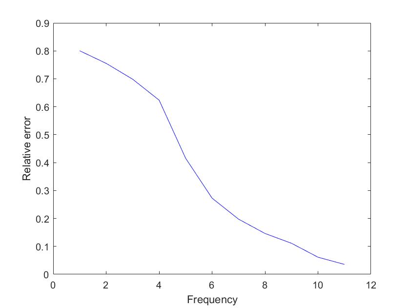 Figure 1
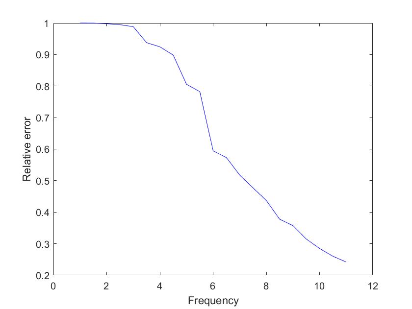 Figure 2
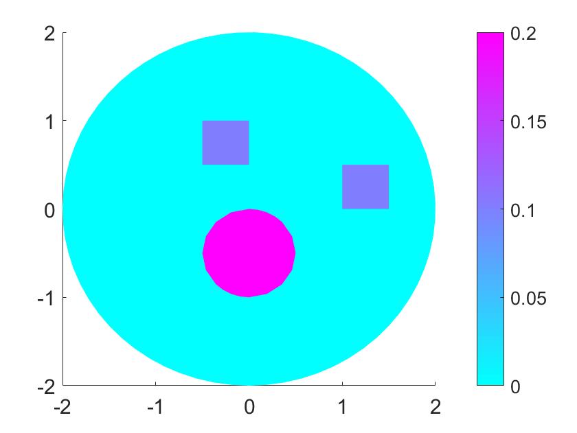 Figure 3
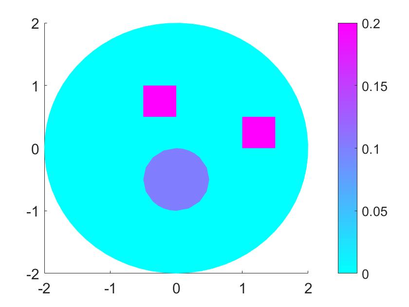 Figure 4
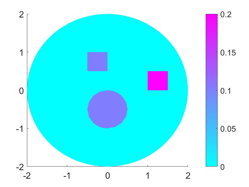 Figure 5
 Figure 6
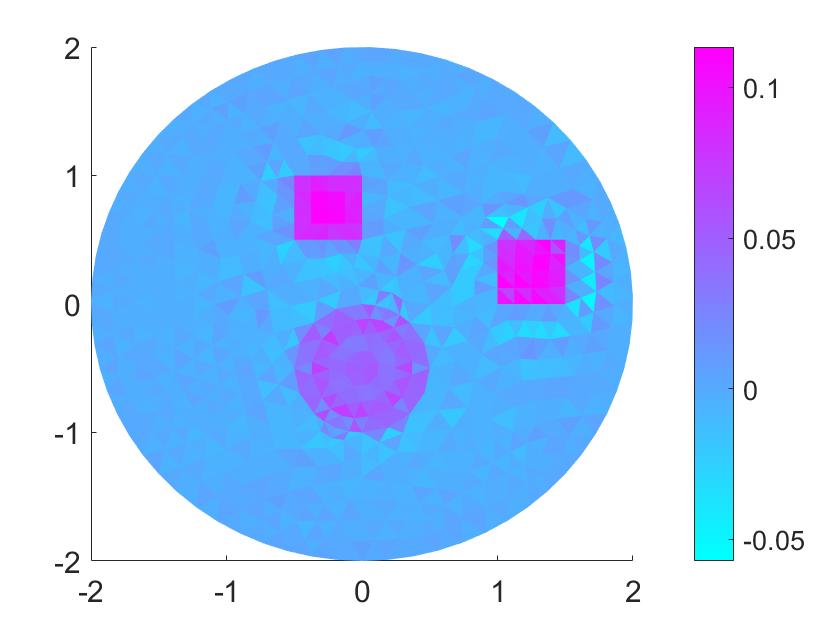 Figure 7
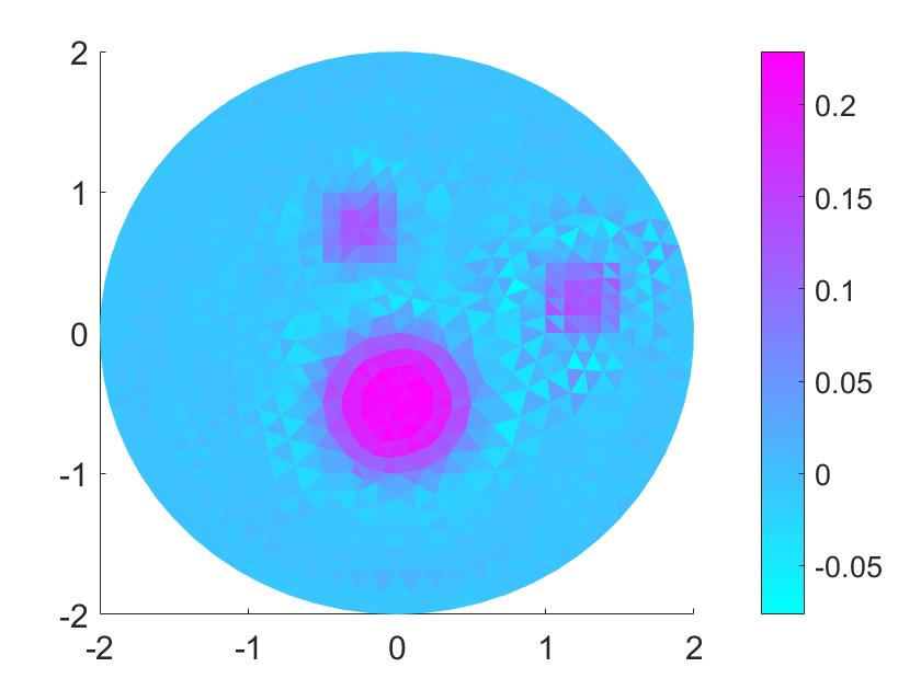 Figure 8
 Figure 9
 Figure 10
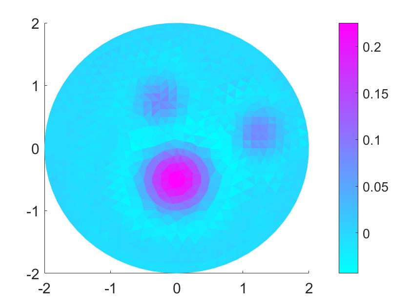 Figure 11
 Figure 12
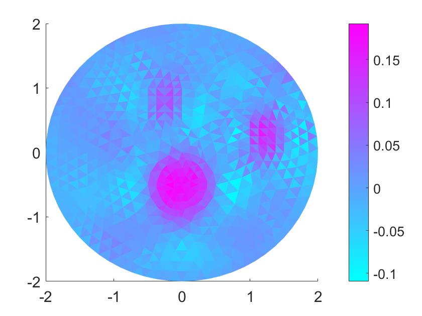 Figure 13
 Figure 14
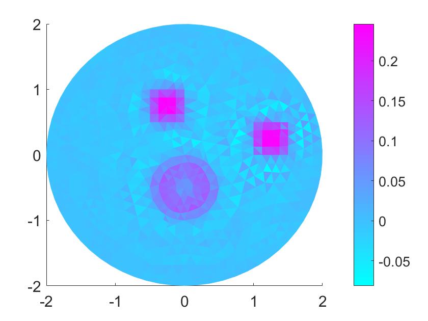 Figure 15
 Figure 16
 Figure 17
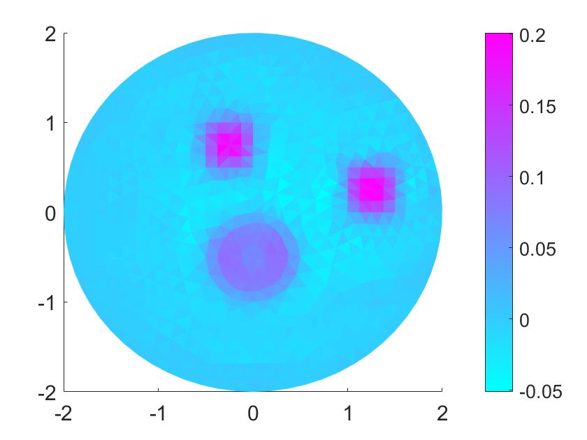 Figure 18
 Figure 19
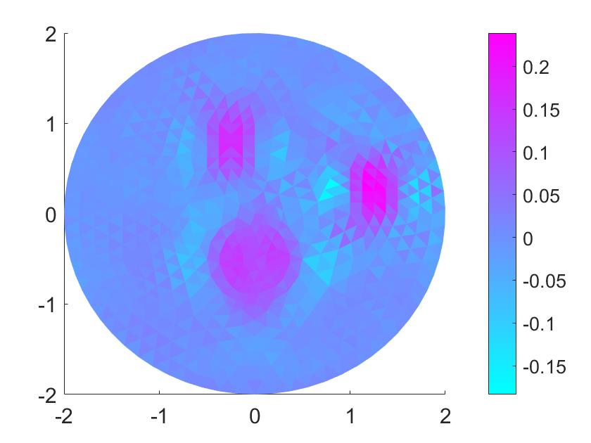 Figure 20
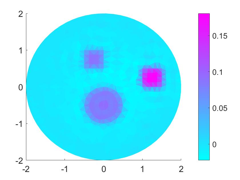 Figure 21
 Figure 22
 Figure 23
 Figure 24
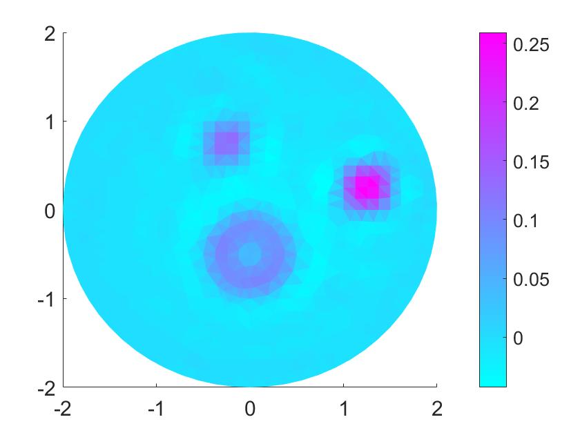 Figure 25
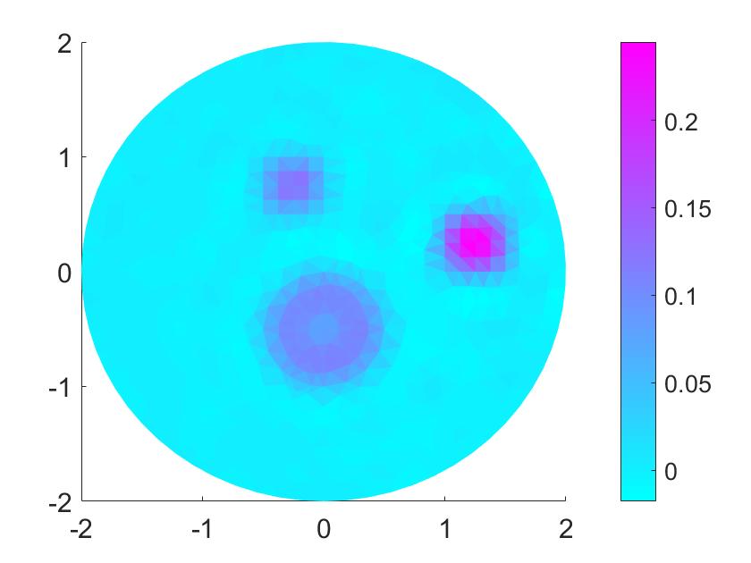 Figure 26
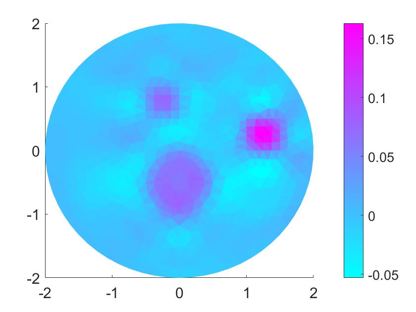 Figure 27
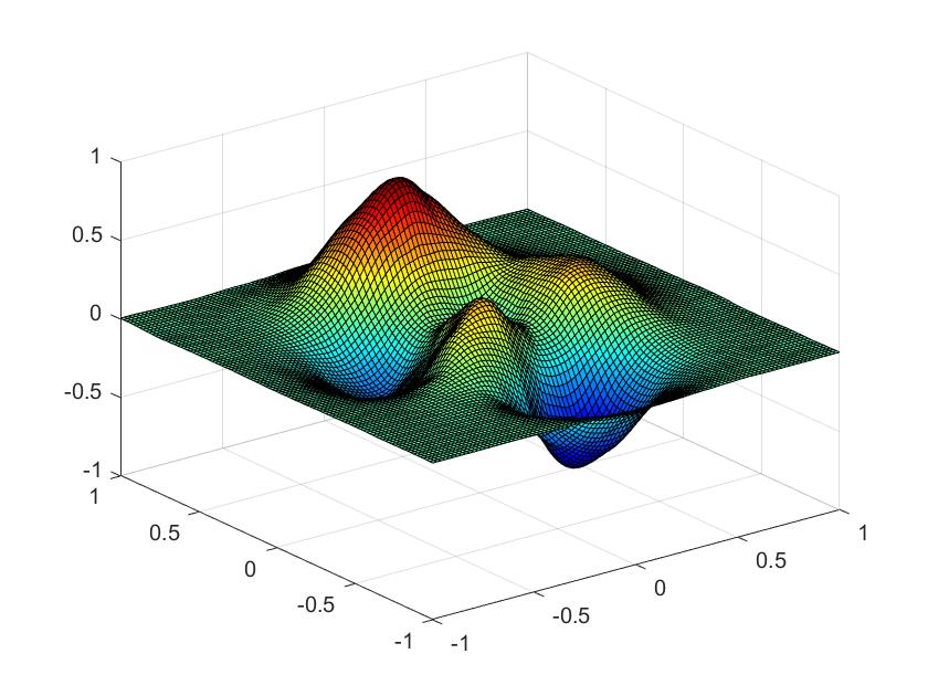 Figure 28
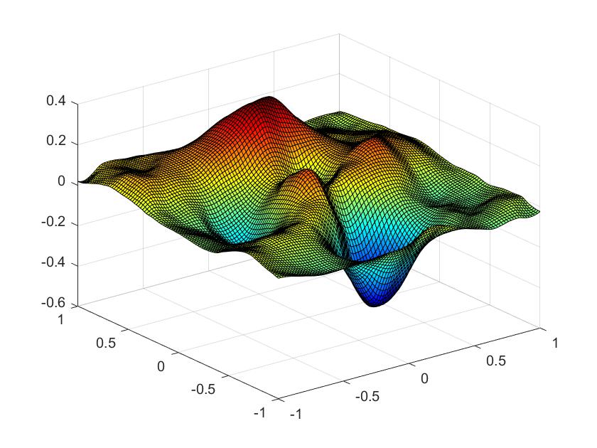 Figure 29
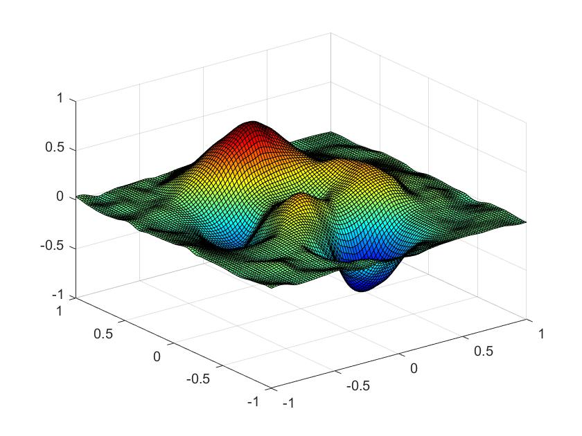 Figure 30
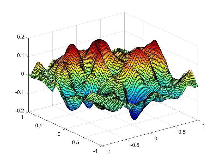 Figure 31
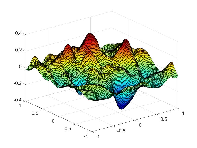 Figure 32
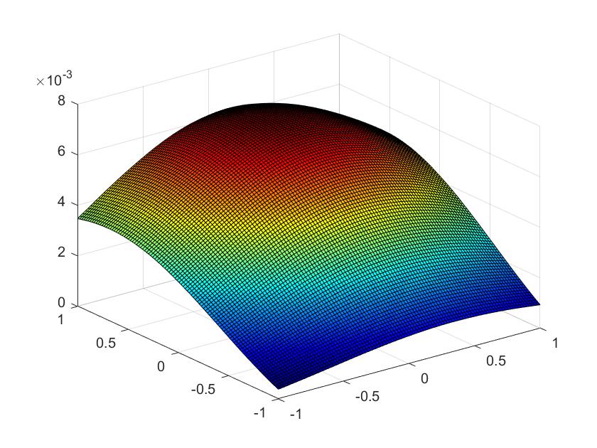 Figure 33
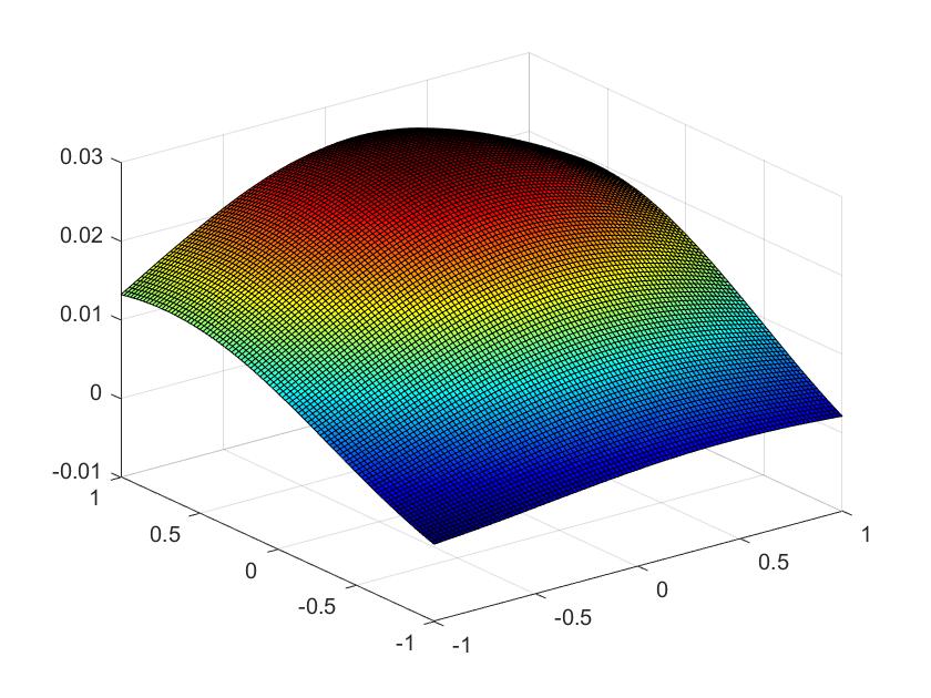 Figure 34
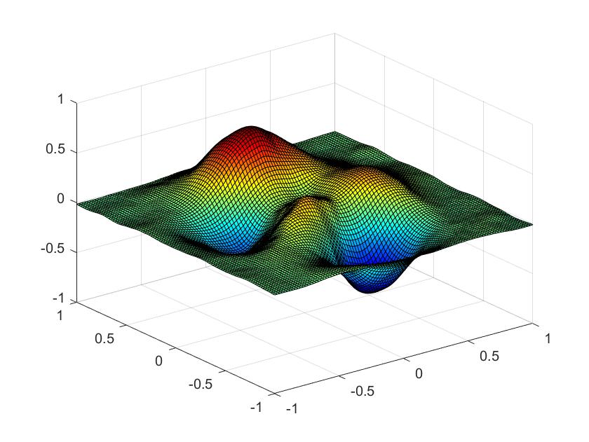 Figure 35
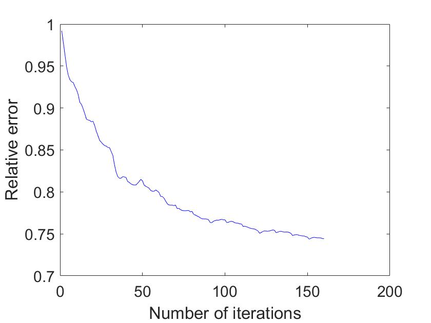 Figure 36
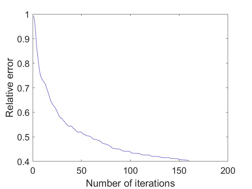 Figure 37
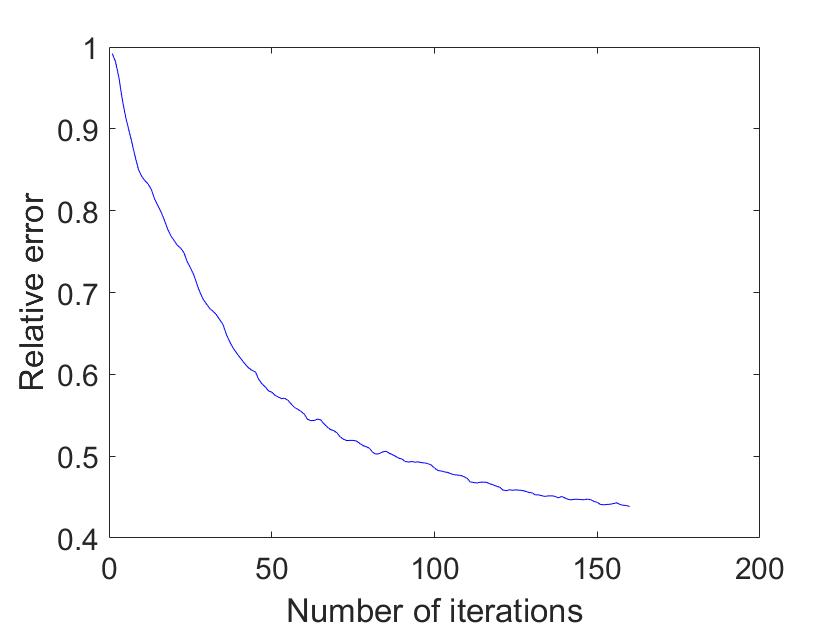 Figure 38
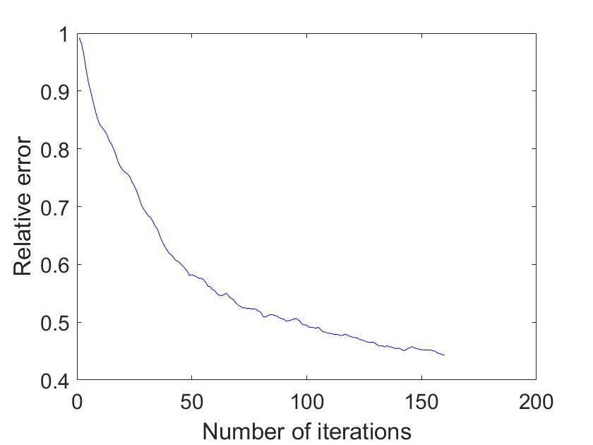 Figure 39
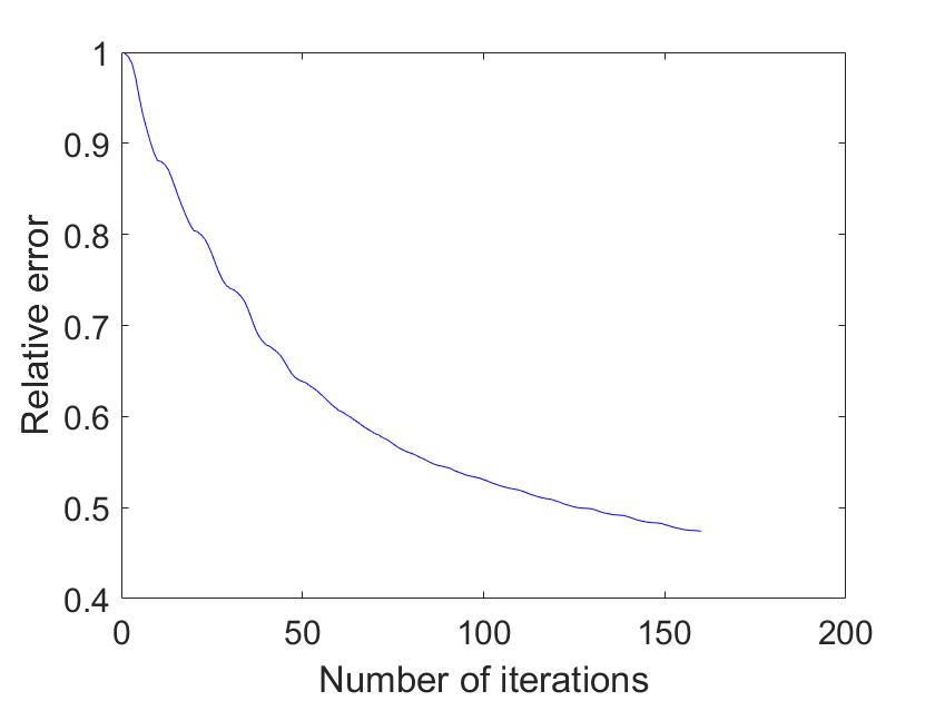 Figure 40
Peer Reviews
No public reviews on file for this paper yet. If you reviewed it on a platform where reviews are public (OpenReview, ICLR, NeurIPS, ICML), you can paste yours below so the community can read it here.
Videos
No videos yet. Explain this paper in a talk, walkthrough, or lecture? Add one.
Taxonomy
TopicsNumerical methods in inverse problems · Microwave Imaging and Scattering Analysis · Ultrasonics and Acoustic Wave Propagation
Abstract
This paper concerns the reconstruction of multiple elastic parameters (Lamé parameters and density) of an inhomogeneous medium embedded in an infinite homogeneous isotropic background in . The direct scattering problem is reduced to an equivalent system on a bounded domain by introducing an exact transparent boundary condition and the wellposedness of the corresponding variational problem is established. The Fréchet differentiability of the near-field scattering map is studied with respect to the elastic parameters. Based on the multi-frequency measurement data and its phaseless term, two Landweber iterative algorithms are developed for the reconstruction of the multiple elastic parameters. Numerical examples, indicating that plane pressure incident wave is a better choice, are presented to show the validity and accuracy of our methods.
Keywords: Elastic wave, inverse medium problem, iterative method, multi-frequency
1 Introduction
Time-harmonic elastic scattering problems play important roles in many fields of applications and the linear elasticity theory provides an essential tool for analysis and design of mechanic systems and engineering structures ([3, 21]). In this paper, we consider several inhomogeneous isotropic elastic bodies embedded in an infinite homogeneous isotropic background medium in . Denote by , the Lamé parameters with , , and by the density of the elastic medium. Suppose that , and where , and are constants representing the Lamé parameters and density of the background elastic medium. Denote and . Set . Throughout, we make the following assumption:
Assumption:
there exists some and constants such that
[TABLE]
Let be a plane incident field satisfying
[TABLE]
where is the frequency and the stress tensor is defined as
[TABLE]
and stands for the identity matrix. The elliptic equation (1.1) can be restated as
[TABLE]
where the Lamé operator is defined as
[TABLE]
In this paper, the incident wave is allowed to be either a plane shear wave taking the form
[TABLE]
or a plane pressure wave taking the form
[TABLE]
where
[TABLE]
are the wave numbers of pressure wave and shear wave, respectively and and are referred as the direction and angle of the incidence, respectively.
The total displacement field can be modeled by the reduced Navier equation
[TABLE]
Since the background medium is unbounded, an appropriate radiation condition at infinity must be imposed on the scattered field to ensure well-posedness of the scattering problem. The scattered field in can be decomposed into the sum of the compressional (longitudinal) part and the shear (transversal) part as follows :
[TABLE]
where the two-dimensional operators curl and are defined respectively by
[TABLE]
It then follows from the decompositions in (1.3) that
[TABLE]
The scattered field is required to satisfy the Kupradze radiation condition (see e.g. [31])
[TABLE]
uniformly with respect to all \hat{x}=x/|x|\in{\color[rgb]{0.000,0.000,0.000}\Gamma_{1}}.
Given the incident field , the direct problem is to determine the scattered field for the known elastic parameters . In practice, the original boundary value problem for the Lamé system can be reduced to an equivalent system on a bounded domain via introducing an exact transparent boundary condition (TBC) on an artificial boundary enclosing the inhomogeneous bodies. The TBC can be formulated by the so-called Dirichlet-to-Neumann (DtN) map taking in the form of a Fourier series ([8, 23, 32, 33]). Based on the properties of the DtN map and Fredholm alternative theorem, the uniqueness and existence of weak solutions of the equivalent system can be derived(Section 2, Theorem 2.4).
The main purpose of this paper is to study numerical algorithm for the inverse medium problem in the elastic scattering, that is, to determine the unknown elastic parameters from the measurements of near-field data , given the incident field . For static case, i.e., , uniqueness of the inverse medium problem has been investigated under appropriate assumptions on the elastic parameters in [2, 18, 22, 28, 35, 37, 36]. For the time-harmonic case, Beretta et al ([19]) proves uniqueness when the Lamé parameters and the density are assumed to be piecewise constant on a given domain partition. For the mathematical analysis of the stability for the inverse medium problems in elasticity, we refer to [1, 18, 27, 35, 36, 37].
Recently, it has been realized that the use of multi-frequency data is an effective approach to overcome the major difficulties associated with the inverse medium problems: the ill-posedness and the presence of many local minima. Based on the multi-frequency measurements and the Fréchet derivative of the solution operator, a stable recursive linearization method is proposed in [10] for the inverse medium problems in acoustics, see also in [12, 11, 13, 14]. The idea to use multi-frequency data has also been widely developed in proving uniqueness and increasing stability for inverse source problems in acoustics, elastodynamics and electromagnetics ([9, 5, 15, 6, 16, 20, 26, 29, 34, 33]). It still remains open whether or not the multi-frequency measurements uniquely determine the Lamé parameters and the density? This paper is designed to study the capability of iterative methods for inverse medium problems in elasticity using multi-frequency measurements. Compared with the acoustic and electromagnetic case, the elasticity problem appears to be more complicated because of the coexistence of pressure and shear waves that propagate at different speeds and the aim to reconstruct multiple parameters. In particular, if the Lamé parameters are constants, the inverse medium problem in elasticity is consistent with that in acoustics, see Section 4. Relying on the variational arguments for the direct problems, we derive the Fréchet derivative of the solution operator with respect to the elastic parameters and investigate the adjoint of the Fréchet derivative. Then we employ the Landweber iterative method based on the multi-frequency measurements to find the unknown elastic parameters. At each iteration step, the forward problem and an adjoint one need to be solved and the correctness of the parameters needs to be evaluated.
The outline of the paper is as follows. In Section 2, we derive the well-posedness of the direct scattering problem using variational approach and investigate the Fréchet differentiability of the near-field scattering map. We develop the Landweber iterative methods for solving the inverse medium problem in Section 3. In Section 4, we give a brief discussion about a special case that . Numerical examples are presented in Section 5.
2 Direct scattering problem
In this section, we discuss the well-posedness of the direct elastic scattering problem and investigate the Fréchet differentiability of the near-field scattering map.
2.1 Variational formulation
We first reduce the original scattering problem described in section 1 on a bounded domain via introducing a TBC on an artificial boundary enclosing the inhomogeneity inside. The TBC is formulated by the so-called DtN map defined as follows.
Definition 2.1**.**
For any , The DtN map applied to is defined as , where satisfies
[TABLE]
and the Kupradze radiation condition. Here, is the traction operator defined by
[TABLE]
where denotes the exterior unit normal vector to and the corresponding tangential vector is given by .
The DtN map is well-defined since the Dirichlet-kind boundary value problem (2.1)-(2.2) is uniquely solvable in , see Corollary 2.3 in [8]. For all , denote
[TABLE]
where
[TABLE]
Following the procedure described in [8], it can be derived that
[TABLE]
where the matrix dependent on the angle is defined as
[TABLE]
and the coefficient matrix is given by
[TABLE]
with
[TABLE]
For the invertibility of matrix , we refer to Lemma 2.11 in [8]. Denote by the determinant of .
Lemma 2.2**.**
For all , the DtN mapping can be expressed equivalently as
[TABLE]
In addition, it holds that
[TABLE]
Proof.
We first prove (2.6). We can derive that for all ,
[TABLE]
where is the duality pairing between and . It remains to prove (2.5). It follows from (2.3) that
[TABLE]
where
[TABLE]
with
[TABLE]
It follows from the properties of Hankel function that
[TABLE]
giving rise to the identities
[TABLE]
From the expressions of and we get the entries of , given by (see also Lemma 2.13 in [8])
[TABLE]
Then we can obtain that , and . These further imply that which completes the proof. ∎
The following property of the coefficient matrix can be obtained directly from Lemma 2.13 in [8].
Lemma 2.3**.**
The matrix is positive definite for sufficiently large .
Using the DtN map, we can impose the following TBC for the scattered field
[TABLE]
Note that
[TABLE]
Then the original scattering problem is equivalently reduced to the following nonlocal boundary value problem
[TABLE]
where . Then the variational formulation of (2.7)-(2.8) reads as follows: find such that
[TABLE]
where the sesquilinear form is defined by
[TABLE]
and
[TABLE]
The double dot notation appeared in is understood in the following way. If tensors and have rectangular Cartesian components and , , respectively, then the double contraction of and is
[TABLE]
The well-posedness of the variational formulation (2.9) is a consequence of the following theorem.
Theorem 2.4**.**
For any and , there exists a unique weak solution to the boundary value problem
[TABLE]
and
[TABLE]
where is a constant independent of .
Proof.
We know from Lemma 2.3 that is positive definite for large . The operator can be decomposed into the sum of an operator whose real part is positive definite and a finite rank operator from to . Define the sesquilinear form as
[TABLE]
Then the variational equation corresponding to (2.11)-(2.12) reads:
[TABLE]
We split the sequilinear form into the sum , where
[TABLE]
Recalling the Korn’s inequality (see e.g. [25]), we have
[TABLE]
with some constant . Moreover, applying the Cauchy-Schwarz inequality yields
[TABLE]
for some constant . From the compact imbedding and the compactness of , we conclude that the sesquilinear form is strongly elliptic (see Definition 2.5) over . The sesquilinear form obviously generates a continuous linear operator such that
[TABLE]
Here denotes the dual space of with respect to the duality extending the scalar product in . We know from the Rellich’s lemma in elasticity (see Lemma 2.14 in [8]) that the homogeneous operator equation has only the trivial solution . Then it follows from the Fredholm alternative that the variational formulation (2.9) is uniquely solvable. Finally, the inf-sup condition
[TABLE]
with some constant generated from the general theory in Babuška and Aziz[4] implies the estimate (2.13). In fact, for , considering the operator equation related to the variational equation (2.14), it follows from the Babuška’s theory that the operator equation is well-posed if and only if the conditions
[TABLE]
and
[TABLE]
hold and they are equivalent to the uniqueness and existence of solution of the operator equation, respectively. Then it follows from the variational equation (2.14) and trace theorem that
[TABLE]
which completes the proof. ∎
Definition 2.5**.**
A bounded sesquilinear form on some Hilbert space is called strongly elliptic if there exists a compact form such that
[TABLE]
2.2 Near-field scattering map
For given perturbed parameters , we define the scattering operator by , where is the unique weak solution of (2.7)-(2.8). It is easily seen that the map is nonlinear with respect to . A direct application of Theorem 2.4 gives the following result.
Lemma 2.6**.**
The map is bounded with the estimate
[TABLE]
where is a constant.
Lemma 2.7**.**
Given the perturbed parameters , , we have the estimate
[TABLE]
where is the the unique weak solution of the problem (2.7)-(2.8) with perturbed parameters and is a constant.
Proof.
Let be the unique weak solutions of the problem (2.7)-(2.8) with perturbed parameters and , respectively. Set . Then we have,
[TABLE]
Then the the inf-sup condition (2.15) together with the boundedness of implies the desired estimate. ∎
For any , assume that is the unique weak solution of the following variational problem
[TABLE]
Let the map be such that
[TABLE]
Lemma 2.8**.**
Given the perturbed parameters , we have the estimate
[TABLE]
where is a constant.
Proof.
Let be the unique weak solutions of the problem (2.7)-(2.8) with perturbed parameters and , respectively. Let , it follows that
[TABLE]
Then we have the estimate
[TABLE]
where is a constant defined as
[TABLE]
∎
Let be the trace operator to the boundary and define the near-field scattering map as . By combining Lemmas 2.6-2.8, we arrive at the following theorem.
Theorem 2.9**.**
The near-field scattering map is Fréchet differentiable with respect to and its Fréchet derivative is .
3 Inverse medium problem
In this section, we consider the inverse medium scattering problem of reconstructing the unknown perturbed elastic parameters and develop a Landweber iterative method. Assume that the total-field data is available over a range of frequencies which can be divided into and over a range of incident directions which can be divided into . Let be the unique solution of the direct scattering problem with and . Consider the following inverse medium problem:
(IP): Given the elastic parameters and of the background medium, reconstruct the perturbed Lamé parameters and perturbed density from the multi-frequency measurements , , .
The inverse problem (IP) can be formulated as: Given and , find and such that
[TABLE]
In particular, the nonlinearity and ill-posedness of the inverse problem cause mathematical challenges from both theoretical and computational points of view. The nonlinearity leads to a nonconvex optimization problem, and the ill-posedness requires certain form of regularization to get a reasonable approximation. Here, to solve the operator equation (3.1) we apply the Landweber iteration method taking the form ([24])
[TABLE]
where is the step size parameter.
3.1 Multi-frequency iterative algorithm
For the adjoint of the operator , we have the following result.
Theorem 3.1**.**
Let be the unique weak solution of (2.7)-(2.8). Then for any ,
[TABLE]
where is the unique weak solution of the following boundary value problem
[TABLE]
Proof.
For any , let be the unique weak solution of the following variational problem
[TABLE]
Replacing by , we obtain
[TABLE]
in which we have used the relation (2.6) and denotes the duality pairing between and . Since it holds for any , we complete the proof. ∎
Denote
[TABLE]
where the index are related to the frequency , the incident direction and the current inner Landweber iteration number. Given initial guesses , we now describe a procedure that determines a better approximation at the frequency with incident direction for , in an increasing manner. For each , we apply steps of Landweber iterations, i.e., . For fixed , suppose now that an approximation of the scatterer has been recovered. For the recovered scatterer , we solve at and the direct problem
[TABLE]
Then for any ,
[TABLE]
where is the unique weak solution of the following boundary value problem
[TABLE]
Then the Landweber iteration leads to
[TABLE]
Note that the elastic parameters are all real values. Therefore, at each step of iterations, we apply a simple regularization as
[TABLE]
The multi-frequency iterative algorithm for solving the inverse medium scattering is summarized in Algorithm 3.1.
Algorithm 3.1 (Multi-frequency iterative algorithm).
- •
Collect the near-field data over all frequencies , and all incident directions , .
- •
Set initial approximations .
- •
Apply the following iteration:
DO
DO
DO
Update the elastic parameters by the formula
[TABLE]
ENDDO
Set
ENDDO
Set
ENDDO
3.2 Multifrequency iterative algorithm from phaseless data
We now consider the reconstruction from phaseless data. Define the phaseless near-field scattering map by
[TABLE]
Lemma 3.2**.**
The phaseless near-field scattering map is Fréchet differentiable with respect to and its Fréchet derivative is given by
[TABLE]
The adjoint of is given in the following Theorem.
Theorem 3.3**.**
Let be the unique weak solution of (2.7)-(2.8). Then for any ,
[TABLE]
where is the unique weak solution of the following boundary value problem
[TABLE]
Proof.
The proof is similar as Theorem 3.1 and we omit it here. ∎
We now describe the Landweber iterative algorithm based on phaseless data. Use the same notations in section 3.1. For any , let be the unique weak solution of the following boundary value problem
[TABLE]
Then the Landweber iteration leads to
[TABLE]
We conclude the algorithm for solving the inverse medium scattering from phaseless data is summarized in Algorithm 3.2.
Algorithm 3.2 (Multi-frequency iterative algorithm for phaseless data).
- •
Collect the near-field data over all frequencies , and all incident directions , .
- •
Set initial approximations .
- •
Apply the following iteration:
DO
DO
DO
Update the elastic parameters by the formula
[TABLE]
ENDDO
Set
ENDDO
Set
ENDDO
3.3 Convergence
In this section, we briefly discuss the convergence of the proposed algorithms based on the classical analysis of Landweber iteration method for nonlinear ill-posed problems. For more detailed analysis of the Landweber iteration and its modification form, we refer to [24, 30] and the references therein. It should be pointed out that although we apply the multi-frequency strategy in this paper, it is extremely difficult to investigate the dependence of the convergence of the algorithms on the number and interval of the selected frequencies. For the corresponding analysis of the inverse medium scattering problems in acoustics that take a similar form as the special case discussed in section 4, we refer to [17].
We consider the following operator equation
[TABLE]
where and are all Hilbert spaces with inner products and norms , respectively. In particular, in this paper. As mentioned above, the operator equation (3.6) is strictly nonlinear and ill-posed. For simplicity, denote . Then the nonlinear Landweber iteration takes the form
[TABLE]
for exact data and the form
[TABLE]
for inexact data satisfying . Here, assume that we take the frequency as the innermost loop.
Let denote a closed ball of radius around . Assume that is sufficiently small such that in . For simplicity, we consider and . Resulting from the regularity theory, we can obtain that , for any small such that , which implies that . Thus, the operator here is compact. According to the analysis in Lemma 2.8 and inverse trace theorem, let and satisfying with sufficiently small , it holds that
[TABLE]
The convergence of the Landweber iteration is given in the following theorem, see Corollary 2.3 and Theorem 2.4 in [30].
Theorem 3.4**.**
Assume that is solvable in . Then the nonlinear Landweber iteration (3.7) converges to a solution of . Furthermore, if for all , then converges to as .
In case of inexact data, the iteration procedure should be combined with a stopping rule in order to act as a regularization method. For example, for each frequency, one can employ the discrepancy principle, i.e., the iteration is stopped after steps with
[TABLE]
where is an appropriately chosen positive number. Before stating the convergence of the iteration (3.8) for inexact data case, we need to discuss the selection of . Note that the parameter must be dependent on .
Proposition 3.5**.**
Assume has a solution and .
- (i).
A sufficient condition for generated from (3.8) to be a better approximation of than is that
[TABLE]
This further leads to the selection of as
[TABLE]
- (ii).
At each frequency, let be chosen according to the stopping rule, we have
[TABLE]
Proof.
The proof is similar to that of the Proposition 2.2 and Corollary 2.3 in [30]. In fact, from (2.13) in [30], it holds that
[TABLE]
which completes the proof of (i) under the sufficient condition. Furthermore, the special choice of implies that
[TABLE]
Adding up these inequalities for from 0 through leads to
[TABLE]
Then (ii) can be proved by combining this inequality and the stoping rule. ∎
Now we can have the following convergence result for inexact data, see Theorem 2.6 in [30].
Theorem 3.6**.**
Assume that is solvable in and let be chosen according to the stopping rule. The nonlinear Landweber iteration (3.8) converges to a solution of . If for all , then converges to as .
Remark 3.7**.**
According to the convergence of Landweber iteration, the choice of the initial approximation may affect the efficiency of the algorithms. In fact, in this paper we reconstruct the relative factors of the elastic parameters of the inhomogeneous medium compared with the parameters of the background medium, not the elastic parameters of the inhomogeneous medium themselves, i.e., we reconstruct
[TABLE]
and they are of . Thus, a simple choice of the initial approximation, that we applied in this paper, is which means that there is no inhomogeneity and it can be seen from the numerical examples that this choice works well. As suggested in [5] for the inverse medium problems in acoustics, one can obtain an initial guess from the Born approximation and the scattering data with the higher frequency must be used in order to recover more Fourier modes of the true scatterer.
4 Discussion of a special case
In this section, we briefly discuss the special case that . In this case, the considered inverse medium problem in elasticity is consistent with that in acoustics and electromagnetics discussed in [10, 12, 11, 13, 14].
Alternatively, one can consider near-field scattering map as \widetilde{N}(q_{\rho})={\color[rgb]{0.000,0.000,0.000}\widetilde{u}}|_{\Gamma_{R}}, where is the unique weak solution of (2.7)-(2.8). Following the steps discussed in sections 2 and 3 (see also in [10]), we can obtain the following result.
Theorem 4.1**.**
The near-field scattering maps are Fréchet differentiable with respect to and their Fréchet derivatives are given by
[TABLE]
where is the unique weak solution of the following boundary value problem
[TABLE]
Moreover, for any ,
[TABLE]
where is the unique weak solution of the following boundary value problem
[TABLE]
Similar as Algorithm 3.1, we can summarize the multi-frequency iterative algorithm for the reconstruction of inhomogeneous density function in Algorithm 3.3.
Algorithm 3.3 (Multi-frequency iterative algorithm for )
- •
Collect the near-field data over all frequencies , and all incident directions , .
- •
Set an initial approximation .
- •
Apply the following iteration:
DO
DO
DO
Update the elastic parameters by the formula
[TABLE]
ENDDO
Set
ENDDO
Set
ENDDO
5 Numerical examples
In this section, we present several numerical examples to verify the accuracy and effectiveness of the recursive algorithm. We always choose , , and . The near-field measurements are obtained by using finite element method solving the forward scattering problem. Define the relative error
[TABLE]
where and are the true and reconstructed values of the parameter of the scatterer. The true values of the elastic parameters are shown in Fig.1. Ten equally spaced frequencies are used in the construction, starting from the lowest frequency and ending at the highest frequency . The number of incident directions is taken as and for . At each incident direction, 10 Landweber iteration steps are taken for one frequency. Corresponding to the stiffness tensor of the background elastic medium using Voigt notation, we chose the relaxation parameter as a matrix
[TABLE]
We collect the final reconstruction error for the following examples in Table 1 and 2. In addition, the number of iterations shown in the following figures are from 0 to .
Example 1. We consider the reconstruction from multi-frequency measurements with multiple incident directions. The reconstructed elastic parameters are presented in Fig.2(a,b,c) and Fig.3(a,b,c). The relative errors shown in Fig.2(d,e,f) and Fig.3(d,e,f) indicate that the relative errors decrease as frequency and number of iteration increase. However, it can be seen that if we choose plane shear incident waves, the reconstruction of , which can further affect the reconstructions of and , is worse than that using plane pressure incident waves. A possible explanation to this phenomenon is that, in comparison with the plane pressure waves, the plane shear incident waves only contain the information of and . In the following, we consider the plane pressure incident waves only. To verify the stability of our method, the reconstructions from noised data with noise levels are presented in Fig.4.
Example 2. Note that one can chose as a scale value. For simplicity, we chose and the reconstruction results and the corresponding relative errors are presented in Fig.5. It can be seen that in this example, the iterations using the step size matrix (5.1) is more stable than those using scale step size. It should be pointed out that we can not prove that using the special choice of step size which looks like the stiffness tensor of the background elastic medium, we can always have better reconstruction than using just a scale one. Our starting pointing is that for isotropic elastic medium, the two Lamé parameters have some connection since they are both determined by the Young’s modulus and Poisson’s ratio and have no direct relation with density. Thus, we take a similar form of stiffness tensor as the choice of step size for example which means that the modification for both , are determined by the combinations of the first two components of and the modification for density is only determined by the third component of . There should be better choices of than the special one we used.
Example 3. In this exampe, we consider the reconstruction from phaseless data. The numerical results are shown in Fig.6 which indicate the effectiveness of our method for the reconstruction from phaseless data.
Example 4. We use the measurements generated by the plane pressure incident wave with one fixed direction (i.e. ). In this case the number of iterations at each frequency is set as . The reconstruction results and relative errors are shown in Fig.7.
Example 5. In this example, we consider the special case discussed in section 4. The exact value of is given by
[TABLE]
see Fig. 8. Choose and . The reconstructed and relative errors from multi-frequency measurements with plane pressure incident wave are shown in Fig.9 and Fig.10.
Example 6. Finally, as a comparison, we consider the reconstruction of mass density only from data at a fixed frequency. For small frequency, it can be seen from Fig.11 that the reconstruction results are extremely bad no matter we have only one or multiple directions of incident wave. But for high frequency, see Fig.12(a), we still can have good reconstruction if we have multiple incident waves. Once we only have one fixed incident wave with direction , we can not obtain good reconstruction result by increasing , see Fig.12(b,c). However, by increasing the number of frequency (), we still can reconstruct some information of , see Fig.13 and the results in Example 4. This further indicate the advantages to take multi-frequency data.
We conclude from the above numerical tests that satisfactory reconstructions are obtained through the proposed Landweber iterative algorithms.
Acknowledgments
The work of G. Bao is supported in part by an NSFC Innovative Group Fund (No.11621101), an Integrated Project of the Major Research Plan of NSFC (No. 91630309), and an NSFC A3 Project (No. 11421110002). The work of F. Zeng is supported by the NSFC grant (No. 11501063, No. 11771068), the Chongqing Research Program of Basic Research and Frontier Technology (No. CSTC2017JCYJAX0294) and the Fundamental Research Funds for the Central University (No. 106112016CDJXY100004). The authors also would like to thank Prof. Peijun Li for his suggestions on this work.
The reference list from the paper itself. Each links out to its DOI / PubMed record.
- 1[1] G. Alessandrini G, M. di Cristo, A. Morassi, E. Rosset, Stable determination of an inclusion in an elastic body by boundary measurements, SIAM J. Math. Anal. 46 (2014) 2692-2729.
- 2[2] M. Akamatsu, G. Nakamura, S. Steinberg, Identification of Lamé coefficients from boundary observations, Inverse Problems 7 (3) (1991) 335-354.
- 3[3] H. Ammari, E. Bretin, J. Garnier, H. Kang, H. Lee and A. Wahab, Mathematical Methods in Elasticity Imaging, Princeton Series in Applied Mathematics, Princeton University Press, 2015.
- 4[4] I. Babuška and A. Aziz, Survey lectures on mathematical foundations of the finite element method. In: A. Aziz(ed.) The Mathematical Foundations of the Finite Element Method with Application to Partial Differential Equations, pp. 5-359. Academic Press, New York, 1972.
- 5[5] G. Bao, P. Li, J. Lin, F. Triki, Inverse scattering problems with multi-frequencies, Inverse Problems, 31 (2015) 093001.
- 6[6] G. Bao, J. Lin, F. Triki, A multi-frequency inverse source problem. J. Differential Equations 249 (2010) 3443-3465.
- 7[7] G. Bao, T. Yin, Recent progress on the study of direct and inverse elastic scattering problems (in Chinese), Sci. Sin. Math. 47 (2017) 1-16.
- 8[8] G. Bao, G. Hu, J. Sun, T. Yin, Direct and inverse elastic scattering from anisotropic media, J. Math. Pures Appl. 117 (2018) 263-301.