Boundary integral equation methods for the elastic and thermoelastic waves in three dimensions
Gang Bao, Liwei Xu, Tao Yin

TL;DR
This paper develops new regularized boundary integral equation formulations for elastic and thermoelastic wave problems in three dimensions, enabling more accurate and efficient numerical solutions using boundary element methods.
Contribution
It introduces novel regularized formulations for hyper-singular boundary integral operators in 3D elastic and thermoelastic wave equations, simplifying numerical computations.
Findings
Regularized formulations reduce singularity complexity.
Numerical examples demonstrate high accuracy.
Effective boundary element method implementation.
Abstract
In this paper, we consider the boundary integral equation (BIE) method for solving the exterior Neumann boundary value problems of elastic and thermoelastic waves in three dimensions based on the Fredholm integral equations of the first kind. The innovative contribution of this work lies in the proposal of the new regularized formulations for the hyper-singular boundary integral operators (BIO) associated with the time-harmonic elastic and thermoelastic wave equations. With the help of the new regularized formulations, we only need to compute the integrals with weak singularities at most in the corresponding variational forms of the boundary integral equations. The accuracy of the regularized formulations is demonstrated through numerical examples using the Galerkin boundary element method (BEM).
Click any figure to enlarge with its caption.
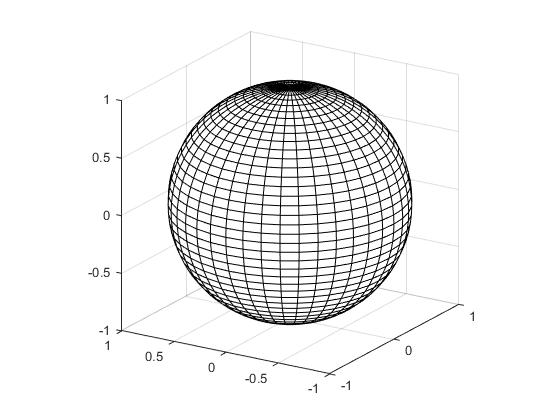 Figure 1
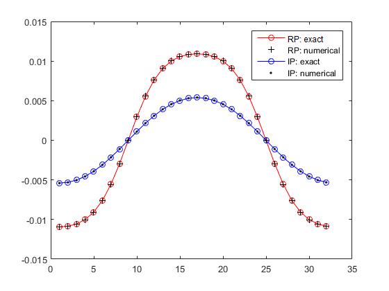 Figure 2
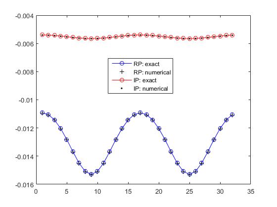 Figure 3
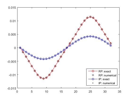 Figure 4
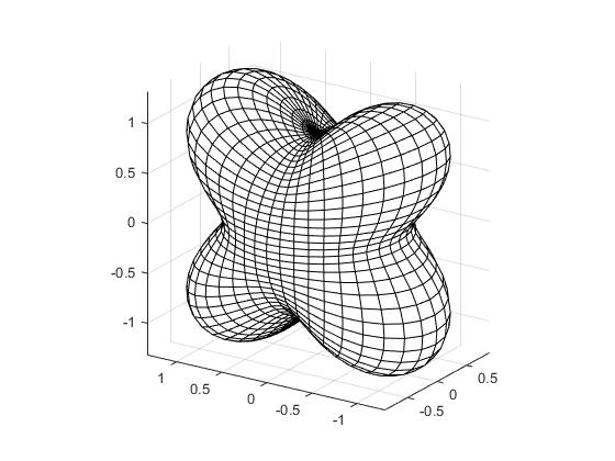 Figure 5
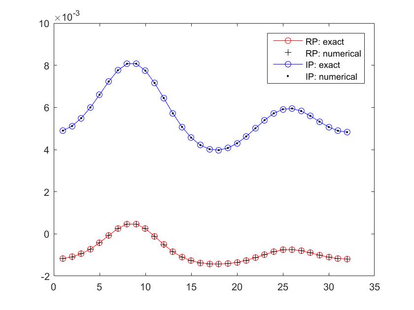 Figure 6
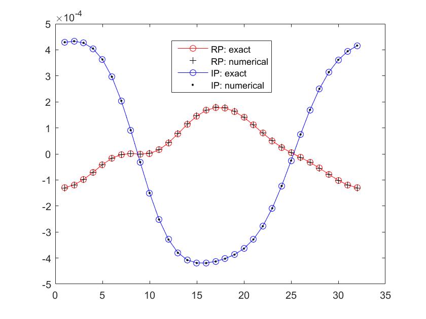 Figure 7
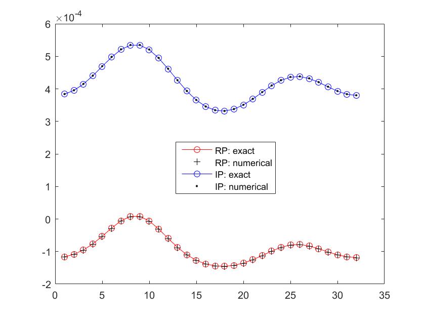 Figure 8
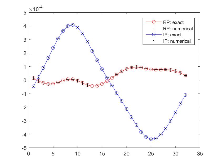 Figure 9
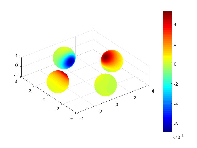 Figure 10
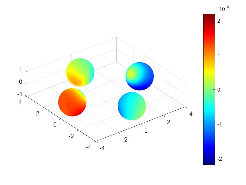 Figure 11
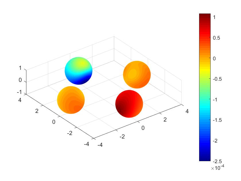 Figure 12
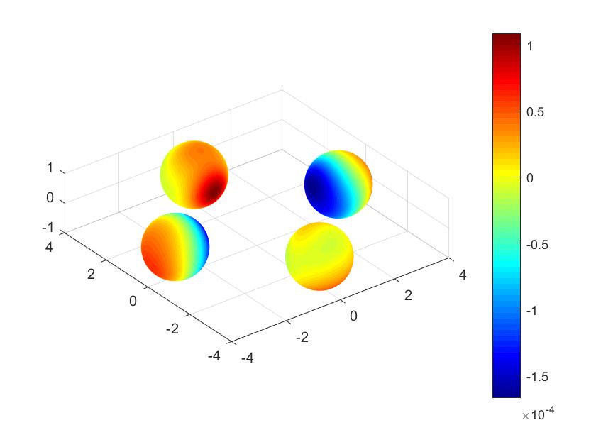 Figure 13
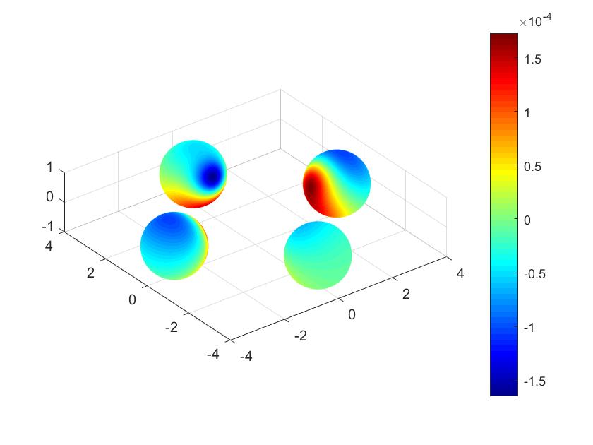 Figure 14
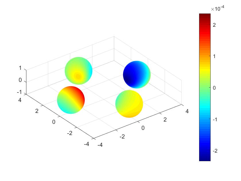 Figure 15
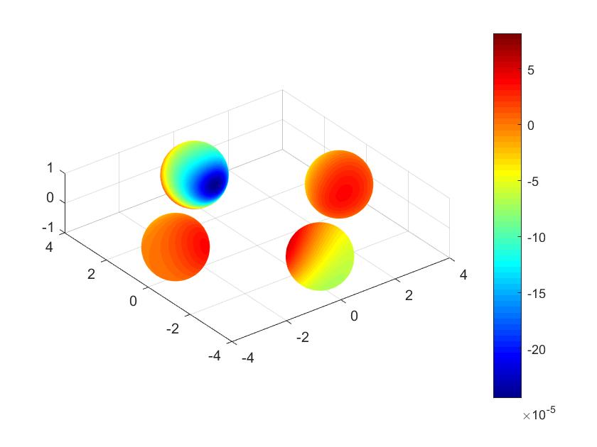 Figure 16
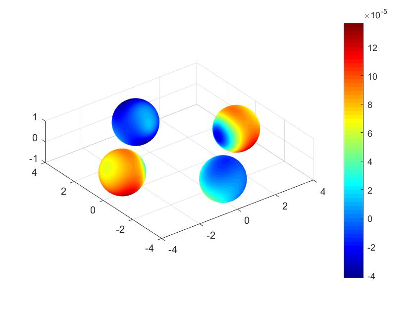 Figure 17
 Figure 18
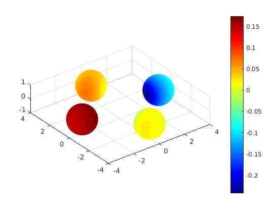 Figure 19
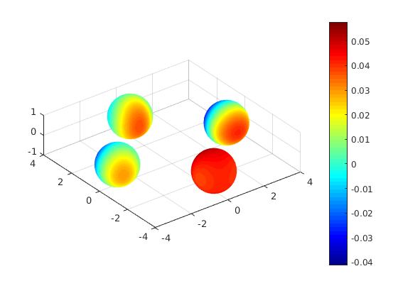 Figure 20
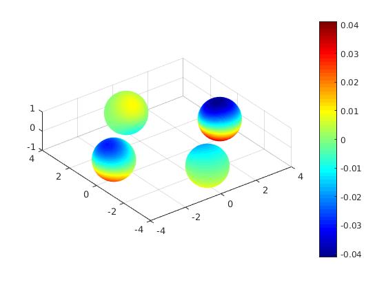 Figure 21
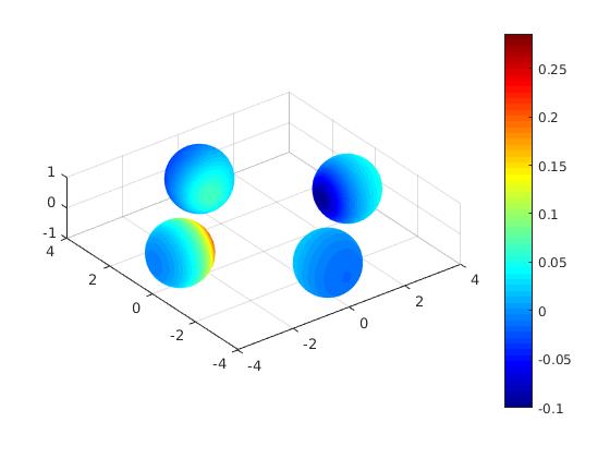 Figure 22
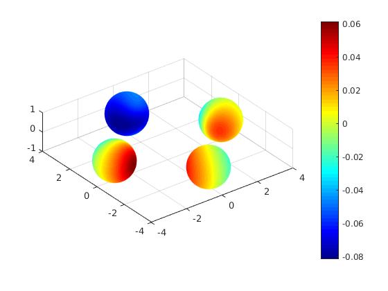 Figure 23
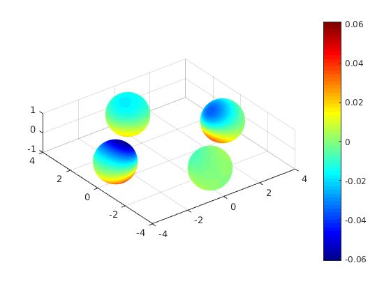 Figure 24
| Error | Order | |
|---|---|---|
| 0.4880 | 1.46E-3 | – |
| 0.3871 | 7.51E-4 | 2.87 |
| 0.2668 | 2.95E-4 | 2.51 |
| 0.1913 | 1.33E-4 | 2.39 |
| 0.1005 | 3.01E-5 | 2.31 |
| Order | ||
|---|---|---|
| 0.4880 | 5.32E-4 | – |
| 0.3871 | 2.22E-4 | 3.77 |
| 0.2668 | 1.07E-4 | 1.96 |
| 0.1913 | 3.59E-5 | 3.28 |
| 0.1005 | 2.61E-6 | 4.07 |
Peer Reviews
No public reviews on file for this paper yet. If you reviewed it on a platform where reviews are public (OpenReview, ICLR, NeurIPS, ICML), you can paste yours below so the community can read it here.
Videos
No videos yet. Explain this paper in a talk, walkthrough, or lecture? Add one.
Abstract
In this paper, we consider the boundary integral equation (BIE) method for solving the exterior Neumann boundary value problems of elastic and thermoelastic waves in three dimensions based on the Fredholm integral equations of the first kind. The innovative contribution of this work lies in the proposal of the new regularized formulations for the hyper-singular boundary integral operators (BIO) associated with the time-harmonic elastic and thermoelastic wave equations. With the help of the new regularized formulations, we only need to compute the integrals with weak singularities at most in the corresponding variational forms of the boundary integral equations. The accuracy of the regularized formulations is demonstrated through numerical examples using the Galerkin boundary element method (BEM).
Keywords: Elastic wave, thermoelastic wave, hyper-singular boundary integral operator, regularized formulation, boundary element method
1 Introduction
In this paper, we apply the BIE method to solve the three dimensional time-harmonic elastic and thermoelastic scattering problems that are of great importance in many fields of applications such as geophysics, seismology, non-destructive testing and material sciences, to name a few. We are interested in the wave scattering by a bounded impenetrable obstacle immersed in an infinite isotropic solid. Based upon the assumption that any deformation of the elastic medium occurs under a constant temperature, the displacement in the solid can be modeled by the Navier equation together with an appropriate radiation condition at infinity ([22]). If considering the temperature fluctuations caused by the dynamic deformation, one arrives at the Biot system of equations ([5, 22, 33]) describing the interaction of the temperature and displacement fields.
When considering the wave propagation in an unbounded domain, one could use the so-called Dirichlet-to-Neumann (DtN) map (or non-reflecting boundary condition) on a closed artificial boundary which decomposes the exterior region into two parts. After that, the original scattering problem could be solved on the bounded region. The DtN map for the elastic wave has been used for numerical simulations in the open literatures ([14, 17]) and some properties of the DtN map have been investigated in [1, 24, 25]. For the thermoelastic wave, the explicit formulation of the DtN map is still unknown. We refer to [8, 9, 12, 13] for the mathematical analysis of the thermoelastic wave. The BIE method is another conventional numerical method for solving the scattering problems, and it has been widely used in acoustics, electromagnetics, elastodynamics and thermoelastodynamics ([4, 2, 7, 10, 11, 18, 19, 20, 21, 23, 27, 26, 28, 31, 34, 35, 36, 37, 38]). The BIE method takes some advantages over domain discretization methods, including that the boundary integral representation of the solution fulfills the radiation condition naturally, the dimension of the computational domain is reduced by one, and to name a few. Various numerical techniques, including the Galerkin scheme, the Nyström method, the fast multipole method, and the spectral method etc., have been developed for the efficient transformation of the BIE into a linear system in the past decades. In this work, we will use the Galerkin scheme ([18, 19, 34]) for the numerical solutions, and its advantages include the availability of mathematical convergence analysis allowing - approximations, and particularly the strength on dealing with the hyper-singularities in the boundary integrals.
During the application of the BIE method, there needs for the use of hyper-singular BIO in many situations, containing the removal of the pollution of eigenfrequencies for the BIE ([6]), and the solution of the Neumann boundary value problem using the Fredholm integral equation of the first kind ([15, 32]), etc.. Theoretical analysis indicates that the hyper-singular BIO is equivalent to the Hadamard finite part of a hyper-singular integral ([19]) which is usually difficult to be calculated accurately. One usually needs additional treatments in numerics for the correct evaluation of the classically non-integrable boundary integrals arising from the hyper-singular BIO. There are already existing many works ([15, 26, 16, 19, 29, 30, 27, 38, 2]) on this issue, and the main idea consists of rewriting the hyper-singular BIO in terms of a composition of differentiation and weakly singular operators for the Laplace equation, the Helmholtz equation, the time-harmonic Navier equation and the Lamé equation. This composition, in fact, is a regularization procedure ([19, 38]) of the hyper-singular distribution, and is useful for the variational formulation and related computational procedures.
In this paper, we consider the three dimensional elastic and thermoelastic scattering problems with Neumann boundary conditions. For each problem, we apply the double-layer potential to represent the solution, and then the original boundary value problem is reduced to a Fredholm boundary integral equation of the first kind with the corresponding hyper-singular BIO. Following the work in [38, 2] for the two-dimensional case, and utilizing the tangential Günter derivative, we derive the new and analytically accurate regularized formulations for the hyper-singular BIO associated with the three dimensional time-harmonic Navier equation and Biot system of linearized thermoelasticity, respectively. As a result, in the corresponding weak forms, all involved integrals are at most weakly-singular. This work is an extension of our work only considering two dimensional elastic waves, and the extension is in fact non-trivial. In the numerical implementations, applying the special local coordinate system given in [34] and the Gauss quadrature rules on the triangle element, we present a semi-analytic strategy to evaluate all the weakly-singular integrals effectively. Although we only consider boundary in our numerical tests, the theoretical results actually could be extended to the Lipschitz case in terms of the properties of Günter derivative given in [3]. The convergence analysis of the numerical scheme could be obtained following the standard techniques in [19], and we will omit it in this work.
The rest of this paper is organized as follows. In Section 2, we introduce the exterior elastic and thermoelastic scattering problems, and then describe the BIE and the Galerkin BEM in Section 3. In section 4, we propose the new and analytically accurate regularized formulations for the hyper-singular BIO in three dimensions. Finally, we discuss a semi-analytic strategy for the numerical implementation of the Galerkin scheme and present numerical results of several examples in section 5.
2 Mathematical problems
Let be a bounded, simply connected and impenetrable body with boundary . The exterior complement of is denoted by . Assume that is occupied by a linear and isotropic elastic solid characterized by the Lamé constants and (, ) and mass density . Let be the frequency of propagating waves.
2.1 Elastic scattering problem (ESP)
Assume that the temperature is always a constant and suppress the time-harmonic dependence . Then the displacement field in the solid can be modeled by the following exterior ESP: Given , determine satisfying
[TABLE]
and the Kupradze radiation condition ([22])
[TABLE]
uniformly with respect to all . Here, is the Lamé operator defined by
[TABLE]
and the traction operator on the boundary is defined as
[TABLE]
where is the outward unit normal to the boundary and is the normal derivative. In (2.3), and are referred as the compressional wave and the shear wave, respectively, and they are given by
[TABLE]
where the wave numbers are defined as
[TABLE]
with
[TABLE]
For the uniqueness of the ESP (2.1)-(2.3), we refer to [22, 1].
2.2 Thermoelastic scattering problem (TESP)
Now we consider the temperature fluctuations caused by the dynamic deformation. In this case, the elastic medium is additionally characterized by the coefficient of thermal diffusity and the coupling constants , given by
[TABLE]
respectively, where is the volumetric thermal expansion coefficient, is a reference value of the absolute temperature and is the coefficient of thermal conductivity. Denote by the dimensionless thermoelastic coupling constant which assumes ’small’ positive values for most thermoelastic media and . Suppressing the time-harmonic dependence , the displacement field and the temperature variation field can be modeled by the following Biot system of linearized thermoelasticity
[TABLE]
Rewriting (2.4)-(2.5) into a matrix form, we obtain
[TABLE]
On the boundary of the scatterer, we assume the Neumann boundary condition
[TABLE]
It follows ([22]) that the wave field admits the decomposition
[TABLE]
where the vector displacement fields satisfy the vectorial Helmholtz equations
[TABLE]
with
[TABLE]
and the scalar temperature fields and satisfy the following scalar Helmholtz equations
[TABLE]
Here, the wave numbers , corresponding to the elastothermal and thermoelastic waves respectively, are the roots of the characteristic system
[TABLE]
for which . In particular,
[TABLE]
where
[TABLE]
We assume that the scattered field satisfies the following Kupradze radiation conditions as for and
[TABLE]
The direct TESP to be considered in this paper is to determine the displacement field and the temperature variation field satisfying (2.6), the boundary condition (2.7) and the Kupradze radiation conditions. For given , we refer to [22, 7] for the uniqueness of the direct problem.
3 Numerical method
In this section, we derive the BIE for solving the ESP and TESP, respectively and give a brief introduction to the Galerkin BEM for the discretization of the derived BIE.
3.1 BIE for ESP
For the ESP, it follows from the potential theory ([22]) that the unknown function can be represented as
[TABLE]
where is referred as the double-layer potential and is the fundamental displacement tensor of the time-harmonic Navier equation (2.1) in taking the form
[TABLE]
In (3.2) and the following, denotes the identity matrix, and is the fundamental solution of the Helmholtz equation in with wave number and takes the form
[TABLE]
Operating with the traction operator on (3.1), taking the limits as and applying the jump relations and the boundary condition (2.2) , we arrive at the BIE on
[TABLE]
where is called the hyper-singular BIO defined by
[TABLE]
The standard weak formulation of (3.4) reads: Given , find such that
[TABLE]
Here and in the sequel, denotes the duality pairing between and for .
3.2 BIE for TESP
For the TESP, it follows from the potential theory ([22, 7]) that the unknown function can be represented as
[TABLE]
where is the fundamental solution of the Biot system (2.6) in given by
[TABLE]
with
[TABLE]
and is the corresponding Neumann operator of the adjoint problem of (2.6) taking the form
[TABLE]
Operating with the operator on (3.7), taking the limits as and applying the boundary condition (2.7) , we obtain the BIE on
[TABLE]
where the hyper-singular BIO is defined by
[TABLE]
The standard weak formulation of (3.8) reads: Given , find such that
[TABLE]
Remark 3.1**.**
For the wellposedness of the variational equations (3.6) and (3.10), we refer the readers to [2, 7, 22]. The pollution of eigenfrequencies on the uniqueness can be removed by applying the so-called Burton-Miller formulation, see [2, 6] for example.
3.3 Galerkin BEM
We only propose the Galerkin Scheme for solving ESP, and the corresponding procedure and formulas for TESP are quite similar and will be neglected. Let be a finite dimensional subspace of . Then the Galerkin approximation of (3.4) reads: Given , find satisfying
[TABLE]
In the following, we describe briefly the reduction of the Galerkin equation (3.11) into its discrete linear system of equations.
Let be a uniform boundary element mesh of where each is a plane triangle with vertex ordered counter clockwise. Let be the set of all nodes of the triangulation. Using the reference element
[TABLE]
the point can be parameterized as
[TABLE]
Let be the set of piecewise linear basis functions. We seek the approximate solution
[TABLE]
where are unknown nodal values of at . For the boundary value , we interpolated it as
[TABLE]
where is the mid point of the element and is the set of piecewise constant basis functions. Substituting the interpolation forms into (3.11) and setting as test functions, we arrive at a linear system of equations
[TABLE]
where for , ,
[TABLE]
[TABLE]
[TABLE]
4 Regularized formulation for the hyper-singular BIO
In this section, we derive the new regularized formulations for the hyper-singular BIOs and in three dimensions such that the coefficient matrix ( or ) can be evaluated in a more effective and accurate way. More precisely, using the derived regularized formulations, only classically integrable and weakly-singular integrals are involved in the weak forms of and . Before doing this, we introduce the hyper-singular BIO associated with the Helmholtz equation and the Günter derivatives.
4.1 Hyper-singular BIO for acoustic scattering problem
Consider the Helmholtz equation
[TABLE]
with wave number . Denote by and , the single-layer and hyper-singular BIO defined by
[TABLE]
respectively. It follows from Lemma 1.2.2 in [19] that the hyper-singular BIO can be expressed as
[TABLE]
4.2 Günter derivatives
Now we describe the Günter derivatives that play essential roles in the proof of our main results. Define the operator , whose elements are also called the Günter derivatives, as
[TABLE]
Then the traction operator can be rewritten as
[TABLE]
A direct calculation yields
[TABLE]
Then
[TABLE]
which implies that
[TABLE]
The properties of the operator ([3, 19, 22]) shows that for any scaler fields , vector fields and tensor field , there hold the Stokes formulas
[TABLE]
and
[TABLE]
4.3 Hyper-singular BIO for ESP
We now investigate the operator . Following the results in [27, 38], we have for ,
[TABLE]
and
[TABLE]
Using the Günter derivatives, the hyper-singular operator can be rewritten as
[TABLE]
where
[TABLE]
Theorem 4.1**.**
The hyper-singular BIO in three dimensions can be expressed alternatively as
[TABLE]
*where . *
Proof.
See A. ∎
4.4 Hyper-singular BIO for TESP
Now we consider the operator . Note that the hyper-singular kernel of is
[TABLE]
where
[TABLE]
For and , we have
[TABLE]
where
[TABLE]
Lemma 4.2**.**
For , it follows that
[TABLE]
and
[TABLE]
Proof.
See B. ∎
We first investigate the term . Observe that the first term in is consistent with the the kernel of hyper-singular BIO . For , we have the following regularized formulation.
Theorem 4.3**.**
The hyper-singular operator can be expressed alternatively as
[TABLE]
Here, the constants are given by
[TABLE]
and
[TABLE]
Proof.
See C. ∎
Next we investigate the terms and . We have
Theorem 4.4**.**
The hyper-singular operators and can be expressed as
[TABLE]
and
[TABLE]
*respectively. *
Proof.
It follows that
[TABLE]
and
[TABLE]
which further implies (4.15) by the Stokes formulas (4.6). The proof of (4.16) is similar and we omit it here. ∎
Finally, we investigate the term . From the results for acoustic wave (4.1), we immediately conclude that
Theorem 4.5**.**
The hyper-singular operator can be expressed as
[TABLE]
Remark 4.6**.**
It can be easily verified from the Stokes formulas of Günter derivatives that using the proposed regularized formulations, all the integrals in the corresponding weak forms of and are at most weakly-singular.
5 Numerical tests
In this section, we present several numerical examples to demonstrate the accuracy of the proposed scheme solving the exterior ESP and TESP. We now take the ESP as the model to describe the method for numerical implementations.
5.1 Numerical implementations
Using the weak form of the regularized formulation (4.10), it follows that (3.13) can be retreated as
[TABLE]
in which the entries of the matrix are given by
[TABLE]
In (5.1), all the integrals are at most weakly-singular. It can be obtained from decompositions that the weakly-singular kernels in (5.1) are of types
[TABLE]
To compute the weakly singular integrals efficiently, we apply the special local coordinate system given in [34] to the boundary element with vertex . Define the unit vector . Set and . Then the intersection point can be determined by or equivalently, . Define another unit vector , and the proportional coefficients . Thus, the boundary element can be parameterized as
[TABLE]
Then for , . The outward unit norma to the element is determined by . Moreover, the piecewise linear basis function for the vertex on can be formulated as , and . In addition, using the above parametrisation we have
[TABLE]
or
[TABLE]
Now we present the main computing strategy of the numerical implementation. Set . Corresponding to the piecewise linear basis function on , set
[TABLE]
Using this reorder strategy and the local coordinate system, on . Therefore,
[TABLE]
are all constants.
The nonsingular integrals involved in (5.1) can be approximated by Gaussian quadrature for triangular elements and we only need to consider the following integrals
[TABLE]
which can be numerically computed following the steps described in [34] in a semi-analytic sense.
5.2 Numerical examples
In the numerical tests, the direct solver ’’ in Matlab is employed for solutions of the linear system (3.12). The impenetrable obstacle is set to be a unit ball (see Figure 2 (a)) or star-like (see Figure 2 (b)) with radial function
[TABLE]
For these two obstacles, the origin is in . In our numerical tests, we first compute the unknown potentials and on by solving the variational equations (3.6) and (3.10), respectively and then put them into the solution representations (3.1) and (3.7) to get the numerical solutions and in , i.e.,
[TABLE]
5.2.1 Numerical examples for ESP
Set , , , . Let the exact solution be
[TABLE]
Denote . Define the numerical error
[TABLE]
For simplicity, we use ’RP’ and ’IP’ to stand for ’real part’ and ’imaginary part’, respectively. The exact and numerical solutions on are plotted in Figure 3 for Obstacle I with . We observe that the numerical solutions are in a perfect agreement with the exact ones from the qualitative point of view. In Table 1, we present the numerical errors Error with respect to the meshsize which indicate the asymptotic convergence order . These results verify the accuracy of the regularized formulation for hyper-singular BIO .
Next, we consider the scattering of an incident plane wave taking the form
[TABLE]
by Obstacle II where is the incident direction. In this case, on . We choose and . The real and imaginary parts of the numerical solution on four unit spheres surrounding the obstacle is presented in Figure 4.
5.2.2 Numerical examples for TESP
Choose , , , , , and . The exact solution is set to be
[TABLE]
and . Define the numerical error
[TABLE]
We plot the exact and numerical solutions on in Figure 5 for Obstacle I with . The numerical solutions are in a perfect agreement with the exact ones from the qualitative point of view. In Table 2, we present the numerical errors with respect to the meshsize which also indicate the convergence. These results verify the accuracy of the regularized formulation for hyper-singular BIO .
Finally, we consider the scattering of an incident point source taking the form
[TABLE]
by Obstacle II where is the location of point source. In this case, on . We choose . The real and imaginary parts of the numerical solutions on four unit spheres surrounding the obstacle is presented in Figure 6.
Appendix A Proof of Theorem 4.1
We know from (4.9) that
[TABLE]
where
[TABLE]
Note that
[TABLE]
where
[TABLE]
We obtain from (4.3) that
[TABLE]
From (4.1) we can obtain that
[TABLE]
For , we know from (4.8) that
[TABLE]
[TABLE]
where
[TABLE]
Note that for ,
[TABLE]
We conclude that
[TABLE]
We obtain from the Stokes formula (4.4) that
[TABLE]
On the other hand,
[TABLE]
Thus,
[TABLE]
Finally, since
[TABLE]
we have
[TABLE]
We complete the proof of (4.10) by a combination of (1.1) and (1.5)-(1.7).
Appendix B Proof of Lemma 4.2
For some matrix or vector , we denote and their Cartesian components, respectively. Let
[TABLE]
Then we have
[TABLE]
[TABLE]
and
[TABLE]
Therefore, from (4.2) and (2.1)-(2.3) we have
[TABLE]
Note that
[TABLE]
Hence,
[TABLE]
which completes the proof of (4.12). The proof of (4.13) follows in similar way, and we skip it here.
Appendix C Proof of Theorem 4.3
Following the same steps in A we can obtain that
[TABLE]
On the other hand, we have
[TABLE]
and
[TABLE]
Then we have
[TABLE]
Then (4.14) can be proved by combining (3.1) and (3.2).
Acknowledgments
The work of G. Bao is supported in part by a NSFC Innovative Group Fund (No.11621101), an Integrated Project of the Major Research Plan of NSFC (No. 91630309), and an NSFC A3 Project (No. 11421110002). The work of L. Xu is partially supported by a Key Project of the Major Research Plan of NSFC (No. 91630205), and a NSFC Grant (No. 11771068).
The reference list from the paper itself. Each links out to its DOI / PubMed record.
- 1[1] G. Bao, G. Hu, J. Sun, T. Yin, Direct and inverse elastic scattering from anisotropic media, to appear in J. Math. Pures Appl..
- 2[2] G. Bao, L. Xu, T. Yin, An accurate boundary element method for the exterior elastic scattering problem in two dimensions, J. Comput. Phy. 348 (2017) 343-363.
- 3[3] A. Bendalia, S. Tordeux, Extension of the Günter derivatives to lipschitz domains and application to the boundary potentials of elastic waves, ar Xiv:1611.04362.
- 4[4] F. Bu, J. Lin, F. Reitich, A fast and high-order method for the three-dimensional elastic wave scattering problem, J. Comput. Phy. 258 (2014) 856-870.
- 5[5] M. A. Biot, Thermoelasticity and irreversible thermodynamics, J. Appl. Phys. 27 (1956) 240-253.
- 6[6] A. J. Burton, G. F. Miller, The application of integral equation methods to the numerical solution of some exterior boundary-value problem, Proc. Roy. Soc. London Ser. A 323 (1971) 201-210.
- 7[7] F. Cakoni, Boundary integral method for thermoelastic screen scattering problem in ℝ 3 superscript ℝ 3 {\mathbb{R}}^{3} , Math. Meth. Appl. Sci. 23 (2000) 441-466.
- 8[8] F. Cakoni, G. Dassios, The coated thermoelastic body within a low-frequency elastodynamic field, Int. J. Engng. Sci. 36 (1998) 1815-1838.