Universal low temperature theory of charged black holes with AdS$_2$ horizons
Subir Sachdev

TL;DR
This paper derives a universal low-temperature effective quantum theory for charged AdS black holes with AdS$_2$ horizons, capturing their near-horizon physics and thermodynamics in a 0+1 dimensional framework.
Contribution
It provides a derivation of the universal effective theory from the full Einstein-Maxwell theory, including quantitative couplings consistent with black hole thermodynamics.
Findings
Effective theory is a Schwarzian action with a phase mode.
Couplings match thermodynamic expectations.
Universal description applies to a class of charged AdS black holes.
Abstract
We consider the low temperature quantum theory of a charged black hole of zero temperature horizon radius , in a spacetime which is asymptotically AdS () far from the horizon. At temperatures , the near-horizon geometry is AdS, and the black hole is described by a universal 0+1 dimensional effective quantum theory of time diffeomorphisms with a Schwarzian action, and a phase mode conjugate to the U(1) charge. We obtain this universal 0+1 dimensional effective theory starting from the full -dimensional Einstein-Maxwell theory, while keeping quantitative track of the couplings. The couplings of the effective theory are found to be in agreement with those expected from the thermodynamics of the -dimensional black hole.
Click any figure to enlarge with its caption.
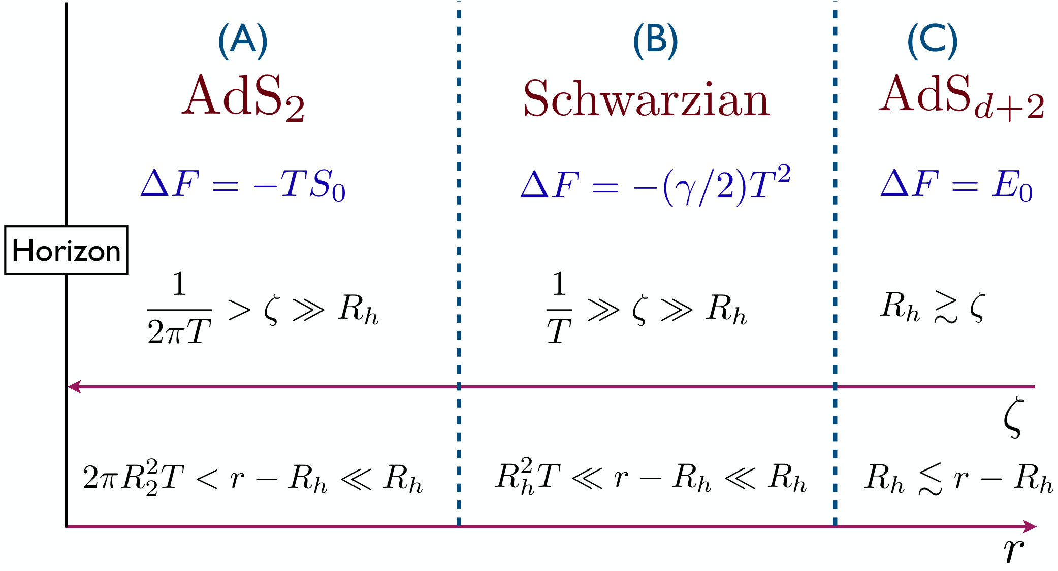 Figure 1
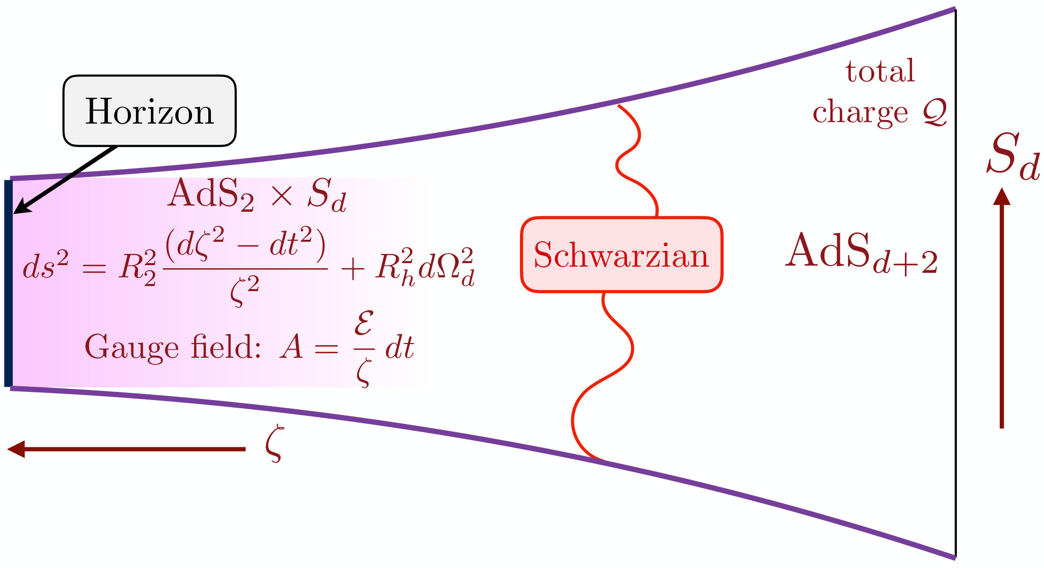 Figure 2
Peer Reviews
No public reviews on file for this paper yet. If you reviewed it on a platform where reviews are public (OpenReview, ICLR, NeurIPS, ICML), you can paste yours below so the community can read it here.
Videos
No videos yet. Explain this paper in a talk, walkthrough, or lecture? Add one.
††institutetext: Department of Physics, Harvard University, Cambridge MA 02138 USA††institutetext: Perimeter Institute for Theoretical Physics, Waterloo, Ontario N2L 2Y5, Canada
Universal low temperature theory of
charged black holes with AdS2 horizons
Subir Sachdev
Abstract
We consider the low temperature quantum theory of a charged black hole of zero temperature horizon radius , in a spacetime which is asymptotically AdSD () far from the horizon. At temperatures , the near-horizon geometry is AdS2, and the black hole is described by a universal 0+1 dimensional effective quantum theory of time diffeomorphisms with a Schwarzian action, and a phase mode conjugate to the U(1) charge. We obtain this universal 0+1 dimensional effective theory starting from the full -dimensional Einstein-Maxwell theory, while keeping quantitative track of the couplings. The couplings of the effective theory are found to be in agreement with those expected from the thermodynamics of the -dimensional black hole.
1 Introduction
Charged black holes in asymptotically AdSD spacetimes have a near-horizon geometry, AdS, where is a compact space, and ; see Fig. 1. The presence of the AdS2 factor implies universal low energy quantum theories for such black holes. At sufficiently low energy scales, non-constant modes on are not excited, and much has been learnt about the resulting theories whose form depends only upon the conserved U(1) charges and the supersymmetry Sen05 ; Dabholkar:2004yr ; Dabholkar:2006tb ; Sen08 ; SS10 ; Dabholkar:2014ema ; AAJP15 ; Alm2016fws ; kitaev2015talk ; SS15 ; JMDS16 ; JMDS16b ; HV16 ; KJ16 ; Fu:2016vas ; Stanford:2017thb ; Davison17 ; Gaikwad:2018dfc ; Nayak:2018qej ; Moitra:2018jqs ; Chaturvedi:2018uov ; Susskindtalk . UV complete theories which realize these low energy limits are found in complex Sachdev-Ye-Kitaev models SY92 ; GPS01 ; SS15 , and they are also expected to appear in the low energy limit of supersymmetric string theories.
A common property of these black holes with charge is that their entropy at low has the form
[TABLE]
where the zero temperature limit is non-zero. The recent advances concern the linear-in- term with co-efficient , which is determined by corrections to the purely AdS2 near-horizon geometry. It has recently been recognized that these corrections are also universal AAJP15 ; Alm2016fws ; JMDS16b , and described by a Schwarzian effective action kitaev2015talk .
For charged black holes, it is also important to consider the variation in the entropy as a function of . In particular, an important dimensionless parameter is , defined by
[TABLE]
The electric field in the near horizon region of the black hole is also determined by Sen05 , as we shall see in Eq. (43). The relationship in Eq. (2) appeared in the context of complex SYK models GPS01 , before also appearing in the black hole context Sen05 , as was recognized later SS15 . The parameter also determines the particle-hole asymmetry of probe matter fields in the AdS2 region: e.g. a fermion of unit charge and scaling dimension has the Green’s function Faulkner09 ; Faulkner:2011tm
[TABLE]
this form applies also to the complex SYK models.
The universal low temperature quantum theory describes both energy and charge fluctuations. It is expressed in terms of a monotonic time diffeomorphism obeying
[TABLE]
and a phase phase field obeying
[TABLE]
integer, which is conjugate to the total integer charge . In the absence of supersymmetry, symmetry arguments lead to the following imaginary time action in the grand canonical ensemble Davison17
[TABLE]
where we have introduced the Schwarzian
[TABLE]
This action is characterized by three parameters, , , and , and these can be specified by their connection to thermodynamics. These parameters depend upon the charge (or the chemical potential ), but this dependence has been left implicit. We have already described the connections of and to the thermodynamics above. The parameter is the zero temperature compressibility
[TABLE]
A different 0+1 dimensional super-Schwarzian action is expected for supersymmetric black holes Fu:2016vas ; Stanford:2017thb , which we will not discuss here.
For neutral black holes connected to the Majorana SYK theory, the 0+1 dimensional theory has allowed non-perturbative computation of the density of low-energy states Cotler:2016fpe ; Garcia-Garcia:2017pzl ; Bagrets:2017pwq ; Stanford:2017thb ; Kitaev:2018wpr . The phase action in Eq. (6) can extend such computations to charged black holes, and this is described in other recent papers GKST19 ; Liu:2019niv . Contrary to early speculations Jensen:2011su , the zero temperature entropy, , is not associated with an exponentially large degeneracy of the ground state (except in cases with supersymmetry Sen05 ; Dabholkar:2004yr ; Sen08 ; Dabholkar:2014ema ; Fu:2016vas ). Instead, there is an exponentially small level spacing down to the ground state, and the envelope of the resulting density of states can be computed from .
This paper will start from the Einstein-Maxwell theory of spherical black holes in asymptotically AdSd+2 space, which we review in Section 2. At low temperatures, such black holes are dominated by fluctuations in the near-horizon AdS2 geometry Faulkner09 , and this is reviewed in our notation in Section 2.1. Section 3 describes a further dimensional reduction from AdS2 to the 0+1 dimensional Schwarzian theory, while keeping quantitative track of all couplings from the parent AdSd+2 theory. This analysis yields the precise co-efficient, , of the Schwarzian action in terms of the couplings in the Einstein-Maxwell theory. This value of is found to be just that expected from a match between the thermodynamics of the black hole in AdSd+2 and the Schwarzian theory.
We turn our attention to the action for the phase mode, , in Eq. (6) in Section 4. Here, we identify with the value of a Wilson line extending from the black hole horizon to the AdSd+2 boundary: see Eq. (63), and also Refs. Nickel:2010pr ; Moitra:2018jqs . We present arguments, based largely on gauge invariance, which lead to a derivation of the term in Eq. (6).
2 Black holes in asymptotically AdS space
We consider the case of spherical black holes in global AdSd+2 (), following the analysis of Chamblin et al. Myers99 . The Einstein-Maxwell theory of a metric and a U(1) gauge flux has Euclidean action
[TABLE]
where is the gravitational constant, is the Ricci scalar, is the radius of AdSd+2, and is a U(1) gauge coupling constant. We will not assume any particular value for the length ratio , and only assume that it is kept fixed as we take the limit. We choose a solution of the saddle-point equations of Eq. (9) with metric
[TABLE]
where is the metric of the -sphere, and
[TABLE]
Note that as , the metric in Eq. (10) is AdSd+2 with boundary geometry ; here is a sphere with a -dimensional surface, and represents the thermal circle.
The gauge field solution has the form
[TABLE]
The equations (10) and (12) solve the Einstein-Maxwell equations provided
[TABLE]
The value of the gauge field at the AdS boundary defines the chemical potential , provided is the horizon. This in turn demands that or
[TABLE]
The temperature of the black hole, , is given by
[TABLE]
The Eqs. (13,14,15) determine all the parameters, , , in terms of and . So we have determined a unique black hole solution in terms of the independent thermodynamic parameters and .
Let us now specify the thermodynamic potentials of the black hole solution. We can compute the grand potential, , by evaluating the action in Eq. (9) for the solution above. However, to obtain a finite answer as the boundary of spacetime at , we have to include boundary counterterms to render the action finite. One of these terms is the familiar Gibbons-Hawking term:
[TABLE]
where the boundary has induced metric , and trace of the extrinsic curvature . In addition, the CFTd+1 residing on the boundary requires local counterterms to obtain a finite action, and these are Henningson:1998ey ; Balasubramanian:1999re ; Myers99a ; Myers99 ; Nayak:2018qej
[TABLE]
where the boundary has Ricci scalar , and we have only shown terms that are needed in . We list the individual contributions of the different actions:
[TABLE]
where is the area of with unit radius. Combining the actions, the terms diverging as cancel, and the grand potential is Myers99
[TABLE]
We can now evaluate the entropy by taking the temperature derivative of to obtain
[TABLE]
which is precisely the expression expected from Hawking’s formula. Similarly, the total charge is obtained by taking the derivative of
[TABLE]
and this expression can also be obtained from Gauss’s law evaluated as
All results above apply for general and , and the and dependence of can be obtained from Eqs. (13,14,15). Let as us now turn to a consideration of the low limit. Explicitly, we have for
[TABLE]
where is the radius the black hole horizon at
[TABLE]
with . Note that the size of the black hole at is determined by the chemical potential alone, and has to be large enough so that the expression inside the square root is positive. We can invert Eq. (23) to write
[TABLE]
For the charge in Eq. (21) we have
[TABLE]
Below we will express all the low thermodynamic parameters of the black hole in terms of . These results can be converted to a dependence on or via Eqs. (25) or (24).
For the grand potential at we obtain
[TABLE]
while the entropy in Eq. (20) is
[TABLE]
We can obtain the function by eliminating between Eqs. (25) and (27). Also we can compute the compressibility
[TABLE]
We also quote another derivative we will need later in Section 4.1
[TABLE]
For the analysis of the low limit, it is better to work at fixed rather than fixed . In the SYK model, the intermediate frequency structure at remains independent of only when we work at fixed PGKS97 ; GPS01 ; SS15 . We will find a similar feature in the low limit of the present black hole solution below. So as , we write
[TABLE]
where
[TABLE]
The first equality in Eq. (31) is the definition of which follows from the expansion in Eq. (30), while the second equality is a general thermodynamic Maxwell relation. We will see below in Eq. (43) that also specifies the electric field at the surface of the black hole. We can compute the value of from the definition in Eq. (31) and Eqs. (13,14,15,21), and obtain
[TABLE]
The ‘equation of state’ obeyed by and is obtained by eliminating between Eqs. (25) and (32); this leads to a lengthy expression which we shall not write out explicitly. But, we can use Eqs. (25), (27) and (32) to verify the identity in Eq. (2)
[TABLE]
Using Eq. (30), we can compute the variation of the entropy at fixed , and so obtain
[TABLE]
We will match this to the co-efficient of the Schwarzian below in Eqs. (47) and (59).
2.1 Dimensional reduction
As illustrated in Figs. 1 and 2, the black hole solution exhibits interesting crossovers in the near-horizon region, when
[TABLE]
Throughout we will assume that the AdSd+2 radius, is held fixed as is lowered. So we take the limit at fixed, but arbitrary, .
It is useful to introduce the co-ordinate via
[TABLE]
so that the horizon will be at . We choose the length scale to be
[TABLE]
and the reason for this specific choice for will become clear below. Note that as , is fixed, and we assume in this subsection that we are in the near-horizon region defined by (see Fig. 2)
[TABLE]
Now we insert the co-ordinate change (36) in the metric (10), and expand in powers of while assuming . Before performing this expansion it is important that we fix the charge of the black hole at also at Faulkner09 . This requires that the chemical potential acquires the -dependence in Eq. (30). With this -dependent , we find that the metric takes the form
[TABLE]
This metric is AdS at . But there is a co-ordinate transformation which maps the metric to the metric for AdS2: we map the co-ordinates to co-ordinates via
[TABLE]
Then the metric for is just as in Eq. (39) but with . Also note that for small , the co-ordinate transformation becomes
[TABLE]
We see from Eq. (39) that the horizon at non-zero is at , and we are interested in the near-horizon region (A) in Fig. 2
[TABLE]
Note also the prefactor of in Eq. (39); the value of was chosen in Eq. (37) by anticipating this prefactor.
Turning to the gauge field sector, the solution in Eq. (12) has the form
[TABLE]
where the dimensionless electric field is exactly equal to that obtained from the definition in Eq. (31). This can also be mapped onto the gauge field via the co-ordinate transformation in Eq. (40), but after a gauge transformation Faulkner:2011tm . Explicitly, let us write in the co-ordinate system at , . Then
[TABLE]
and can be computed from Eq. (40). We perform a gauge transformation generated by to obtain , . In this manner, we obtain , and as in Eq. (43), provided we choose
[TABLE]
It is useful to write out some of the thermodynamic parameters in terms of the parameters of the AdS Sd geometry, but independent of , the radius of AdSd+2. We can write the charge in Eq. (25) as
[TABLE]
which is the expression expected from application of Gauss’s law at the horizon using Eqs. (39,43). And the linear-in- term in the entropy in Eq. (34) can be written as
[TABLE]
Although there is no corresponding expression for which is independent of , we do have the relation
[TABLE]
The expression in Eq. (48) relates the chemical potential to the work done by a unit charge moving from the horizon to the boundary.
We emphasize that the relations in Eqs. (46,47,48) hold at arbitrary values of the ratio .
3 The Schwarzian action
Section 2.1 described the reduction of the spacetime metric from dimensions, a form which factorized spacetime into 2 and dimensions. Fluctuations in the -dimensional space, which is a sphere of radius , are expected to be subdominant for . In this section we will perform the equivalent reduction in terms of the action, to an effective quantum gravity theory in 2 dimensions. Then we will follow Maldacena et al. JMDS16b and further reduce the two-dimensional gravity to a one-dimensional Schwarzian action.
We write the -dimensional metric of in Eq. (9) in terms of a two-dimensional metric and a scalar field Davison17 ; Nayak:2018qej :
[TABLE]
Both and , and the gauge field , are allowed to be general functions of the two-dimensional co-ordinates and . To begin with, we do not specialize to just the near-horizon region, and so there are no restrictions on the value of other than it is outside the horizon; from Eq. (36) the latter constraint is . The boundary of the spacetime is at , corresponding to . Then the expressions for the Einstein-Maxwell (Eq. (9)) and Gibbons-Hawking (Eq. (16)) actions reduce to ()
[TABLE]
along with an additional term not displayed which cancels in Nayak:2018qej . The Gibbons-Hawking term is to be evaluated at the boundary at or . Here is the two-dimensional Ricci scalar, the second integral is over a one-dimensional boundary with metric and extrinsic curvature . The powers of in Eq. (49) were judiciously chosen so that there would be no gradient of in Eq. (50), and that would couple to . The explicit forms of the potentials and are,
[TABLE]
The two-dimensional action in Eqs. (50,51) has exactly the same saddle point solution as that of the four-dimensional action in Eq. (9), and this solution can be obtained by mapping Eq. (49) to Eq. (10). In particular, we obtain from this solution using Eqs. (10) and (36) the exact expression for the saddle point value of
[TABLE]
This scalar field profile will be a key ingredient in the derivation of the Schwarzian action below.
The next step is to renormalize the theory in Eq. (51) down to the near horizon region so that the spacetime is in the region defined by Eq. (42), and the boundary of spacetime is at a in region (B) of Fig. 2
[TABLE]
This moving of the boundary will induce a complicated renormalization of the potentials and , but it will turn out that we will not need the explicit form of this renormalization. The boundary term in Eq. (50) will now be evaluated at . Note that the counterterms, , in Eq. (17) all vanish when evaluated at a one-dimensional boundary with spatial dimensions: so they have no counterpart for two-dimensional gravity. Nevertheless, in computing the free energy of the theory in Eq. (50), the countributions of have to be included, and computed in the full dimensional theory as . However, after renormalizing to the boundary at , no remaining contributions from are needed. Also, such counterterms are not needed for the action in Eq. (50) to yield consistent local equations of motion.
We already know from Section 2.1 that the saddle point metric in the near-horizon region is AdS2. In the form in Eq. (49), the two-dimensional metric is scaled by factor from that in Eq. (39):
[TABLE]
Also in the near-horizon regions (A) and (B), the field coupling to , which in our case is , has the saddle point obtained from Eq. (52)
[TABLE]
with the coefficients
[TABLE]
Note that in the entire AdS2 region, including both its bulk (A) and its boundary (B), as in Fig. 2. The solution with and the metric in Eq. (54) describes the near-horizon AdS region (A) in Fig. 2, and we are interested in the structure of the corrections from to this leading order result.
One of the remarkable observations of Almheiri and Polchinski AAJP15 and Maldacena et al. JMDS16b is that the action for quantum fluctuations with these corrections, with general , is universal. More specifically, they argued that the field coupling to must have the saddle point spatial dependence in Eq. (55), and that the action for the quantum fluctuations reduces to a boundary action in region (B) dependent only upon the value of in Eq. (55). The independence of the bulk action in region (A) on the correction in Eq. (55) follows from the first order variation in the action in Eq. (50), which vanishes because of the bulk equation of motion for
[TABLE]
The result in Eq. (57) is easily verified after employing the AdS2 metric in Eq. (54), the near-horizon gauge field in Eq. (43), and potentials in Eq. (51).
Another important observation of Maldacena et al. JMDS16b is that quantum fluctuations about the metric in Eq. (54) can be represented entirely by fluctuations of a quantum boundary theory (such as the complex SYK model). In the bulk inside the boundary, the metric remains fixed at that in Eq. (54), and the induced metric on the boundary is fixed at . The fluctuations of the boundary theory are realized by a boundary time diffeomorphism, which also determines the shape of the boundary embedded in AdS2. Before determining the action for such fluctuations, we change notation for the bulk time from to , and use as the symbol for the parametric time along the boundary. Then the boundary curve is at bulk co-ordinates . The boundary metric induced by Eq. (54) equals after we choose, in an expansion in ,
[TABLE]
Finally, we evaluate in Eq. (50) along this boundary curve. As we have already included the contribution of in Eq. (55) at the saddle point, and so we need only include in Eq. (50). In this manner we obtain the action JMDS16b (see Appendix A)
[TABLE]
Note that the function in the last equation is the same as that obtained in Eq. (41) in the co-ordinate mapping from to near the boundary. Comparing with the action in Eq. (6), we obtain
[TABLE]
After using the value of in Eq. (56), we find that this value of is in perfect agreement with the value obtained from the thermodynamics of the Einstein-Maxwell theory in dimensions, which is presented in Eqs. (34) and (47). This is the main result of this section.
We note here that upon evaluating the Schwarzian for , we obtain , which yields a change in the free energy of
[TABLE]
We are working here at constant , and hence contributes to , and not directly to . This result for was indicated in Fig. 2, and its -derivative is in Eq. (1).
4 Effective action for the phase mode
This section will consider gauge fluctuations of the Einstein-Maxwell action in Eq. (9). These correspond to charge fluctuations in the boundary theory, which are represented by a phase field . As in Section 3, we will limit our consideration to in the present section.
We are interested in bulk solutions satisfying the boundary condition
[TABLE]
which is satisfied by Eq. (12). It is useful to consider the more general case in which is time-dependent, as indicated in Eq. (62); but we will ultimately make time independent. The key observation of Son and Nickel Nickel:2010pr (see also Ref. Moitra:2018jqs ) is that there are a family of bulk gauge fields satisfying these boundary conditions. In particular there is a non-trivial Wilson line from the horizon to the boundary which defines the phase field in Eq. (6) with non-trivial dynamics
[TABLE]
Gauge transformations which maintain Eq. (62) only perform a time-independent shift , corresponding to the presence of a globally conserved U(1) on the boundary. So the effective action of for will depend only on , as we will see below.
To derive an effective action for this mode, let us introduce the bulk analogue of this Wilson line
[TABLE]
so that
[TABLE]
The bulk field acts as a proxy for the radial gauge field and approaches the boundary Wilson line as i.e.
[TABLE]
In the presence of a time-dependent , we write the metric in Eqs. (10) as
[TABLE]
where, for now, we allow for arbitrary and dependence in and . Then the Maxwell term in the action in Eq. (9) can be written as
[TABLE]
where we have integrated over the angular co-ordinates. Now let us examine the bulk equation of motion for
[TABLE]
We can determine the function by integrating the second equation to obtain
[TABLE]
This determines in terms of the metric and the combination . We can insert the so determined into the Maxwell action and obtain
[TABLE]
We now need to insert the Maxwell action specified by Eqs. (70) and (71) into Eq. (9), and solve the resulting saddle point equations for the metric obtained from the total action . At zeroth order in , this solution is just that specified by Eq. (10). However, we need to determine the correction to the action to order , and for this we need to include the corrections to the metric which are linear order in ; in the boundary theory, these corrections correspond to perturbations in the stress energy tensor which are sourced by a non-zero . Fortunately, these corrections, and the resulting change in the effective action, can be determined by a simple argument. Notice that the influence of is solely by the shift in Eq. (70). At low frequencies, it is safe to ignore the time-dependence in , and so the shift in the metric is simply proportional to the derivative of the metric (which is non-zero). So we can compute the action by working at a fixed , and then replacing .
The combined contribution to the effective action from fluctuations at is then
[TABLE]
where is the grand potential in Eq. (19). The second term is a total derivative, and the last term has a coefficient which equals the compressibility in Eq. (28).
4.1 Non-zero temperatures
This section describes the extension of the phase action in Eq. (72) to .
At , we have imposed the rigid boundary condition in all our analysis so far, and this fixes the form of to that in Eq. (72). The situation changes at , because the computations in Sections 2.1 and 3 assumed a fixed and a variable , and this required the -dependent change in chemical potential in Eq. (30). In contrast, in Section 4 so far, we are considering the effective action at fixed and variable . In terms of boundary conditions in the AdS/CFT context, these situations correspond to whether we fix the co-efficient of term in Eq. (12) (as in Section 4) or the co-efficient of the term (as in Sections 2.1 and 3) as we vary .
Therefore, we need to supplement the fixed action in Eq. (59), with a fixed action. It is useful to motivate the required action by considering the relationship between the corresponding thermodynamic derivatives. We saw in Eq. (61) that the Schwarzian action computed . Correspondingly, we wish to extend Eq. (72) to compute . But the difference between these two derivatives is specified by thermodynamics:
[TABLE]
We can now assume that both free energies are time integrals of their respective actions, and as above Eq. (72), we momentarily ignore the frequency dependence of the actions. Then we can carry out the mapping in Eq. (73) between the fixed and fixed situations at the level of local effective actions. At order , such an analysis amounts to replacing by the difference in the chemical potential between the two approaches divided by . So we need to take the difference between the chemical potential in the fixed case, i.e. , from that in the fixed case, i.e. as in Eq. (30). Their difference is , and this identifies the required modification of :
[TABLE]
Now at leading order, ignoring phase fluctuations, we obtain a contribution from Eq. (74) to the grand potential of . By Eq. (73) this has to be added to the contribution in Eq. (61), to yield the total order contribution to the grand potential
[TABLE]
It can now be verified that Eqs. (75) and (61) are consistent with Eq. (73), and also with the explicit value of in Eq. (29), after using the values of , , and in Section 2.
4.2 Coupling to the diffeomorphism mode
This section considers the modification of the phase action in Eq. (74) from the boundary time diffeomorphism mode of Section 3.
An important observation, following from the analysis above Eq. (74), is that any coupling of Eq. (74) to a diffeomorphism mode should vanish at . There can be no corrections to Eq. (72) at , apart from a renormalization of the coupling , and the effective action can only depend upon the combination independent of the metric.
In Section 4.1, we argued that we need the chemical potential which keeps fixed at variable for the computation in Section 3. In the absence of diffeomorphisms in time, this was given by Eq. (30). We will now compute the correction to Eq. (30) in the presence of the time diffeomorphism of the boundary theory.
For this computation, we focus on the AdS2 region (A) of Fig. 2. The vector potential is given by Eq. (43), which we write as
[TABLE]
We apply the usual rules of the AdS/CFT correspondence Hartnoll:2016apf at the AdS2 boundary, which is here (but with , see Fig 2). We identify the term in Eq. (76) with the chemical potential at the AdS2 boundary, while the coefficient of the is proportional to the conjugate charge density. Notice also that the form in Eq. (76) is asymptotically consistent with the form in Eq. (12) for AdSd+2 with (after mapping from to via Eq. (36)).
Now let us consider quantum fluctuations on the boundary theory (realized by the complex SYK model), represented by the boundary time diffeomorphism . The chemical potential of the boundary, , transforms like the time component of a vector potential: , and so . The boundary chemical potential in the original time is , and so the chemical potential in the theory with time is .
Having computed the chemical potential at the AdS2 boundary, we need to determine the chemical potential at the AdSd+2 boundary, . In the absence of time diffeomorphisms, these two chemical potentials are connected by Eq. (30). We have already argued that there can be no -independent coupling to the diffeomorphism . Furthermore, leading -dependent renormalization to in Eq. (30) arises entirely from the AdS2 region. So we conclude that the generalization of Eq. (30) is
[TABLE]
Using this renormalized chemical potential in the reasoning above Eq. (74), we obtain the updated action for phase fluctuations
[TABLE]
The full action is therefore , which yields Eq. (6) from Eq. (59).
5 Discussion
The Reissner-Nördstrom-AdS charged black hole has been extensively used as a holographic model of strongly interacting quantum matter at non-zero density Hartnoll:2016apf . Near the boundary, the geometry is AdSD, and so the conventional rules of the AdS/CFT correspondence apply, and they can be used to relate bulk properties to the correlations of the boundary quantum theory in spacetime dimensions. It was also recognized Faulkner09 that (for ) the low temperature correlations are linked to the near-horizon AdS2 geometry. But it had not seemed possible to express the physics in terms of the 2-dimensional bulk alone, without embedding it in a higher-dimensional geometry.
Maldacena et al. JMDS16b recently proposed a novel formulation of the 2-dimensional bulk quantum physics. Following the example of the SYK model, they argued that the strong back reaction of the AdS2 geometry to external perturbations AAJP15 ; Alm2016fws could be accounted for by integrating over a time diffeomorphism () in the quantum theory on the boundary of AdS2. After fixing the induced metric on the boundary of AdS2, the time diffeomorphism determines the shape of the AdS2 boundary. They also obtained a 0+1 dimensional Schwarzian action for the time diffeomorphisms. For the case of a charged black hole, the bulk U(1) gauge field implies that the Schwarzian action has to be supplemented Davison17 by that of a scalar phase field (), leading to the action in Eq. (6). The path integral over this action can be exactly computed Stanford:2017thb ; GKST19 ; Liu:2019niv , and this allows computation of quantum properties beyond what has been possible from the AdSD approach above.
These advances result in two approaches to determining the low temperature correlations of the quantum system holographically equivalent to a charged black hole: we can use the conventional AdS/CFT correspondence at the AdSD boundary, or the Schwarzian theory at the AdS2 boundary (see Fig. 1). Earlier works SS10 ; kitaev2015talk ; SS15 ; JMDS16b ; KJ16 ; HV16 ; Davison17 ; Moitra:2018jqs established the equivalence of the two approaches by comparing thermodynamics and correlation functions. Here, we have derived the effective 0+1 dimensional action as a low energy limit of the Einstein-Maxwell theory of charged black holes in asymptotically AdSD space, and confirmed that the tree-level predictions of the two actions are in precise quantitative agreement. The quantum fluctuation corrections from the 0+1 dimensional effective action can now be applied to the -dimensional Einstein-Maxwell theory. The mapping to the effective theory is valid at temperatures , where is the radius of the black hole. However, we do not assume any particular relation between and the AdSD radius , and our analysis can approach asymptotically Minkowski space for large .
Acknowledgements
This analysis was undertaken for lectures at the 36th Advanced School in Physics at the Israel Institute for Advanced Studies in Jerusalem (lecture videos), and I am grateful to all participants for many stimulating interactions. I thank M. Blake, R. Davison, N. Iqbal, J. Maldacena, G. Mandal, D. Stanford, S. P. Trivedi, and S.R. Wadia for useful discussions. M. Blake and R. Davison contributed to the early stages of the analysis in Section 4. This research was supported by the US Department of Energy under Grant No. DE-SC0019030. Research at Perimeter Institute is supported by the Government of Canada through Industry Canada and by the Province of Ontario through the Ministry of Research and Innovation. I also acknowledges support from Cenovus Energy at Perimeter Institute.
Appendix A Extrinsic curvature and the Schwarzian
We consider a general metric of a two-dimensional space with co-ordinates
[TABLE]
We are interested in the extrinsic curvature of a curve parameterized by : .
Let us transform to new co-ordinates so that the curve is at . For small we choose the co-ordinate transformation
[TABLE]
This insures that the metric in the new co-ordinates is of the Gaussian normal form
[TABLE]
with
[TABLE]
The induced metric on is , and the extrinsic curvature of is
[TABLE]
From Eq. (54), we now use
[TABLE]
and fix the curve by Eq. (58) which sets . Then we evaluate the extrinsic curvature of , expand in powers of , and insert in Eq. (50) with , to obtain Eq. (59). Note (i) all the powers of the metric prefactor cancel out; (ii) in the evaluation of (but not for other quantities), it turns out we only need to keep the leading term of order in Eq. (58).
The reference list from the paper itself. Each links out to its DOI / PubMed record.
- 1(1) A. Sen, Black hole entropy function and the attractor mechanism in higher derivative gravity , JHEP 0509 (2005) 038 , [ hep-th/0506177 ]. · doi ↗
- 2(2) A. Dabholkar, Exact counting of black hole microstates , Phys. Rev. Lett. 94 (2005) 241301 , [ hep-th/0409148 ]. · doi ↗
- 3(3) A. Dabholkar, A. Sen and S. P. Trivedi, Black hole microstates and attractor without supersymmetry , JHEP 01 (2007) 096 , [ hep-th/0611143 ]. · doi ↗
- 4(4) A. Sen, Entropy Function and Ad S(2) / CFT(1) Correspondence , JHEP 0811 (2008) 075 , [ 0805.0095 ]. · doi ↗
- 5(5) S. Sachdev, Holographic metals and the fractionalized Fermi liquid , Phys. Rev. Lett. 105 (2010) 151602 , [ 1006.3794 ]. · doi ↗
- 6(6) A. Dabholkar, J. Gomes and S. Murthy, Nonperturbative black hole entropy and Kloosterman sums , JHEP 03 (2015) 074 , [ 1404.0033 ]. · doi ↗
- 7(7) A. Almheiri and J. Polchinski, Models of Ad S 2 backreaction and holography , JHEP 11 (2015) 014 , [ 1402.6334 ]. · doi ↗
- 8(8) A. Almheiri and B. Kang, Conformal Symmetry Breaking and Thermodynamics of Near-Extremal Black Holes , JHEP 10 (2016) 052 , [ 1606.04108 ]. · doi ↗