Surface waves enhance particle dispersion
Mohammad Farazmand, Themistoklis Sapsis

TL;DR
This study reveals that surface gravity waves cause super-diffusive particle dispersion, with variance growing quadratically over time, significantly faster than traditional linear models predict, due to long-term velocity correlations.
Contribution
The paper demonstrates that surface waves induce super-diffusive dispersion of particles, contrasting with classical models, through exact nonlinear trajectory calculations.
Findings
Particle variance grows as t^2 at large times.
Surface waves significantly enhance particle dispersion.
Long-term velocity correlations cause super-diffusive behavior.
Abstract
We study the horizontal dispersion of passive tracer particles on the free surface of gravity waves in deep water. For random linear waves with the JONSWAP spectrum, the Lagrangian particle trajectories are computed using an exact nonlinear model known as the John--Sclavounos equation. We show that the single-particle dispersion exhibits an unusual super-diffusive behavior. In particular, for large times , the variance of the tracer increases as a quadratic function of time, i.e., . This dispersion is markedly faster than Taylor's single-particle dispersion theory which predicts that the variance of passive tracers grows linearly with time for large . Our results imply that the wave motion significantly enhances the dispersion of fluid particles. We show that this super-diffusive behavior is a result of the long-term…
Click any figure to enlarge with its caption.
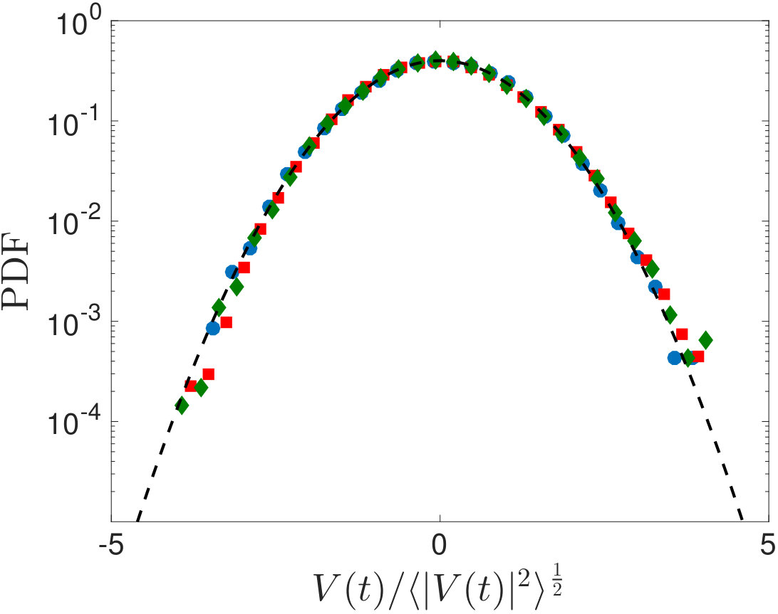 Figure 8
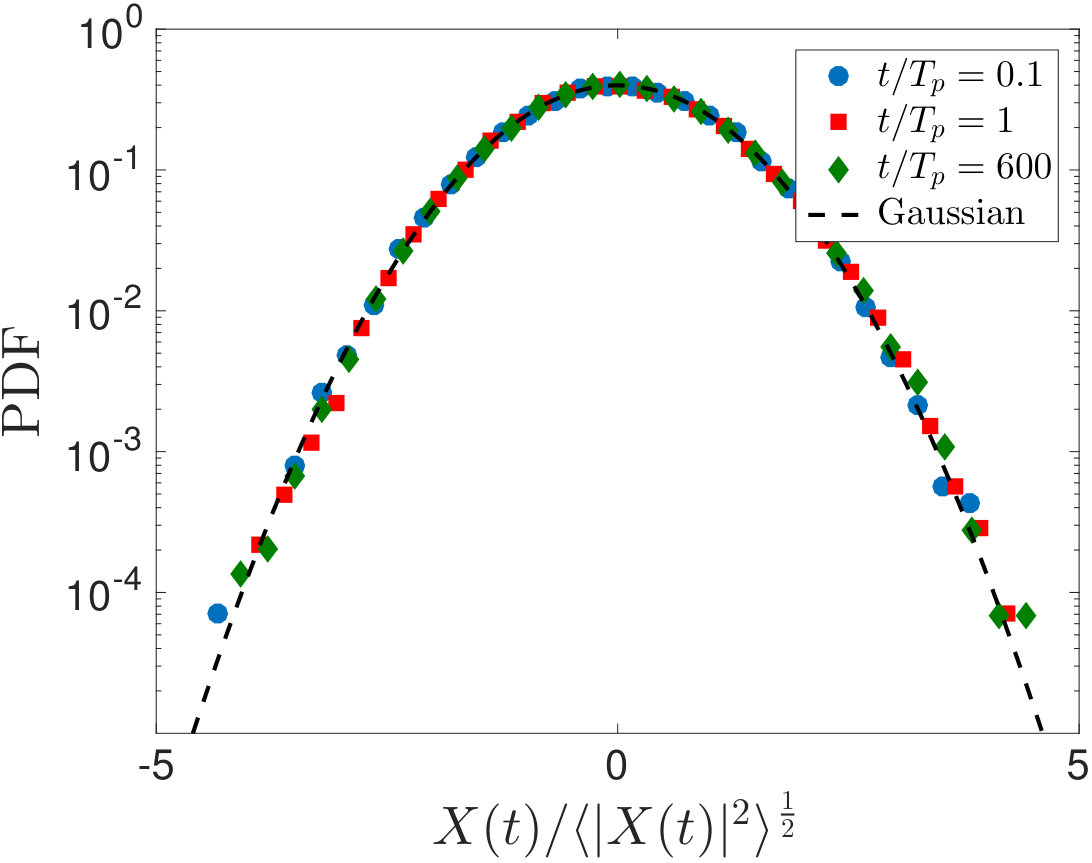 Figure 9
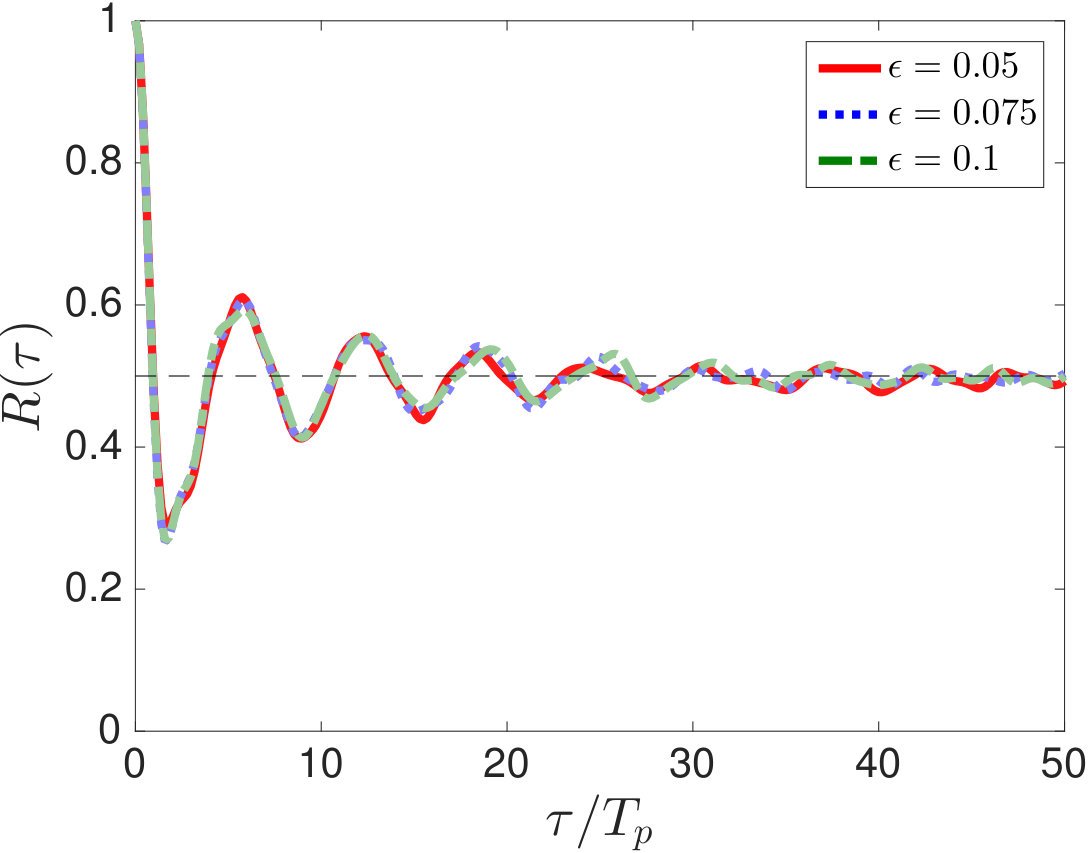 Figure 10
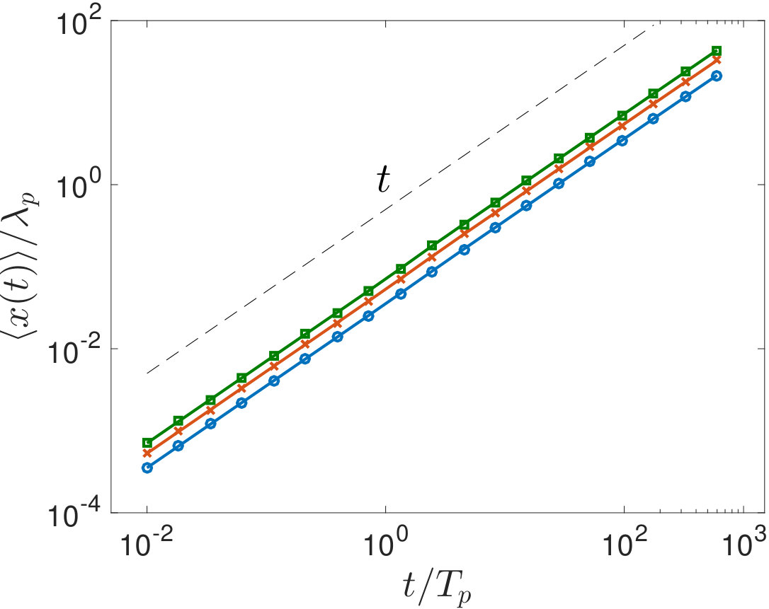 Figure 11
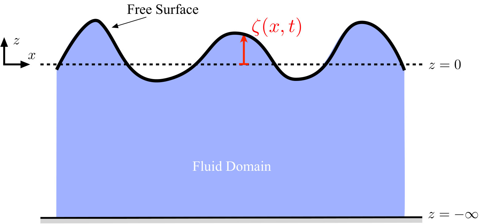 Figure 12
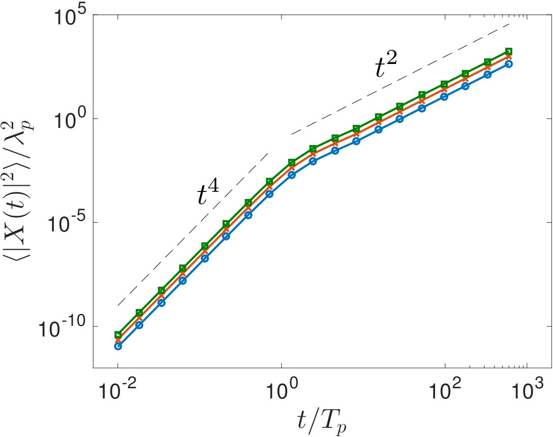 Figure 13
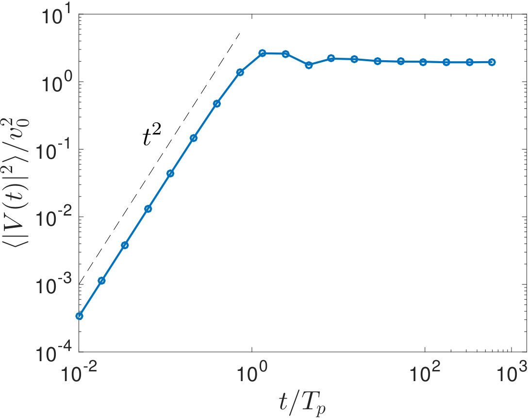 Figure 14
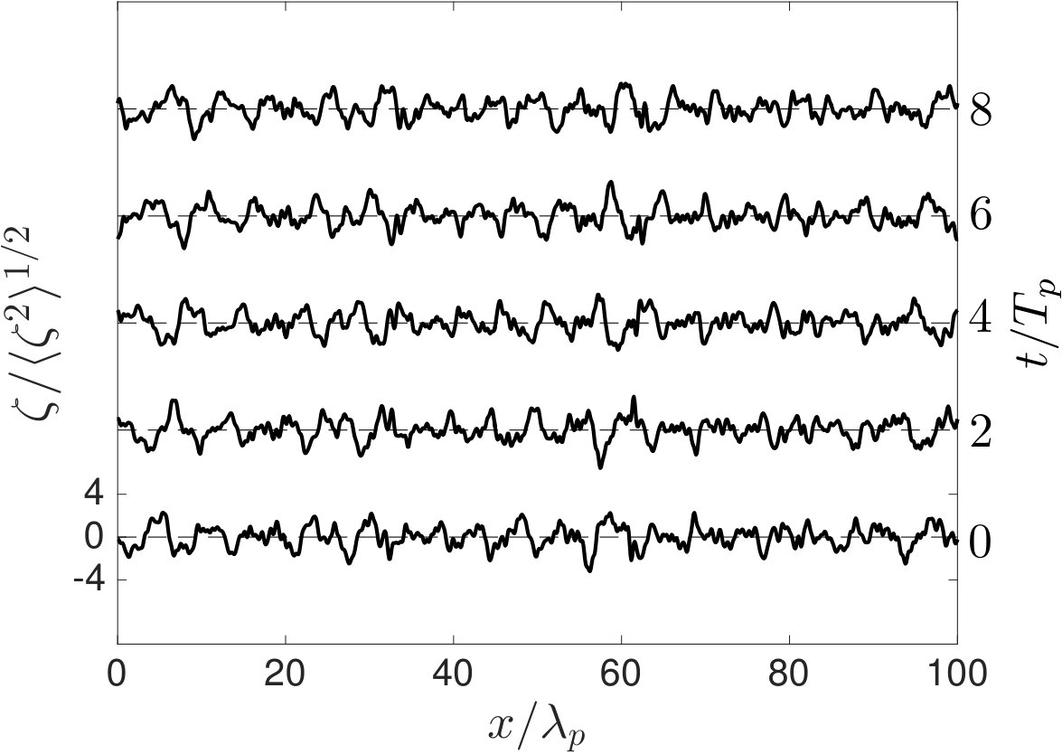 Figure 15
Peer Reviews
No public reviews on file for this paper yet. If you reviewed it on a platform where reviews are public (OpenReview, ICLR, NeurIPS, ICML), you can paste yours below so the community can read it here.
Videos
No videos yet. Explain this paper in a talk, walkthrough, or lecture? Add one.
Taxonomy
TopicsOcean Waves and Remote Sensing · Coastal and Marine Dynamics · Aeolian processes and effects
Abstract
We study the horizontal dispersion of passive tracer particles on the free surface of gravity waves in deep water. For random linear waves with the JONSWAP spectrum, the Lagrangian particle trajectories are computed using an exact nonlinear model known as the John–Sclavounos equation. We show that the single-particle dispersion exhibits an unusual super-diffusive behavior. In particular, for large times , the variance of the tracer increases as a quadratic function of time, i.e., . This dispersion is markedly faster than Taylor’s single-particle dispersion theory which predicts that the variance of passive tracers grows linearly with time for large . Our results imply that the wave motion significantly enhances the dispersion of fluid particles. We show that this super-diffusive behavior is a result of the long-term correlation of the Lagrangian velocities of fluid parcels on the free surface.
keywords:
turbulent dispersion; waves; Stokes drift
\pubvolume
xx \issuenum1 \articlenumber5
\historyReceived: date; Accepted: date; Published: date
\TitleSurface waves enhance particle dispersion \AuthorMohammad Farazmand*∗* \orcidA and Themistoklis Sapsis \AuthorNamesMohammad Farazmand and Themistoklis Sapsis
\corresCorrespondence: [email protected]; Tel.: +1-617-253-5546
1 Introduction
Water waves cause the material transport of fluid particles on the free surface of the fluid. The waves induce a fluid velocity on the free surface which in turn determines the horizontal motion of fluid particles on the free surface. This phenomena has been known since Stokes Stokes (1847) who studied the average velocity of fluid parcels transported by a linear monochromatic wave. The resulting displacement is referred to as the Stokes drift.
More specifically, denote the horizontal trajectory of a fluid particle on the free surface by (or , for short). For simplicity, we assume that the waves are unidirectional. The map denotes the horizontal position of a fluid parcel at time given its initial position at time . The surface elevation is assumed to be a graph over the horizontal coordinates and is denoted by (see figure 1). Since the fluid parcels on the free surface are constrained to it, their vertical position of the parcel is given by . Therefore, knowledge of the horizontal position of the fluid particles and the free surface elevation completely determines the position of the particles.
For a fixed initial condition , Stokes’ theory Stokes (1847) seeks to determine the average displacement of the particles at a later time. Here, denotes the ensemble average over many realizations of the random surface waves. In other words, the Stokes’ theory is concerned with the first-order statistics of the fluid displacement on the free surface. The main focus of the present work is the second-order statistics of particle dispersion. More precisely, we examine the temporal evolution of the variance where denotes the mean-zero displacement of the fluid particles.
1.1 Summary of the main results
As we review in Section 1.2, this second-order statistics has also been studied extensively. However, previous studies either assume the velocity field as a linear superposition of the velocity induced by linear waves or use perturbation theory to approximate the velocity field. Here, however, we obtain the fluid particle trajectories from an exact model known as the John–Sclavounos (JS) equation (see Section 3 for a review). This exact nonlinear kinematic model was first derived by John (1953) for unidirectional irrotational water waves. Sclavounos (2005) generalized the equations to two-dimensional waves and removed the irrotationality assumption. Fedele et al. (2016) further analyzed the JS equation discovering its underlying Hamiltonian structure.
Using the JS equation, we compute the temporal evolution of the variance for fluid particles evolving from a given initial condition . This puts us in the framework of the single-particle dispersion theory. Single-particle dispersion was first studied by Taylor (1922) in the context of homogeneous, isotropic turbulence (see Section 2, for a review). Taylor’s dispersion theory predicts that the variance exhibits a ballistic motion for short times (i.e., ) and a diffusive motion for large times (i.e., ), so that the variance follows the scaling laws
[TABLE]
These scaling laws are often assumed in the study of fluid particles dispersed by surface waves. The main contribution of the present study is to show that Taylor’s dispersion laws (1) may be violated for particles advected by free-surface waves. More precisely, our results can be summarized as follows.
The variance of the particles advected by a surface wave follow the scaling laws
[TABLE]
where denotes the wave period. This is markedly different from the prediction of Taylor’s theory. In particular, the long-term evolution of the variance follows a ballistic motion as opposed to a diffusive motion. 2. 2.
Central to Taylor’s theory of single-particle dispersion is the autocorrelation function of the Lagrangian fluid velocities (see Section 2, for a precise definition of ). To arrive at the scaling laws (1), Taylor assumes that this autocorrelation function decays to zero rapidly enough so that the integral exists and its value is finite. We show, however, that for particles dispersed by surface waves, the autocorrelation function decays to as . This observation, in turn, explains the unusual scaling (2).
1.2 Earlier studies
Previous studies of particle dispersion on the free surface of a fluid can be divided into three general categories: i) Passive tracers on a flat free surface, ii) Linear or nonlinear waves with the induced velocity field modeled based on simplifying assumptions, and iii) Velocity field derived from satellite altimetry data.
The first category is concerned with the Lagrangian motion of fluid particles on the flat free surface of a fluid in a container. Although the three-dimensional flow is incompressible, the velocity field restricted to the surface can be compressible. As a result, the passive tracers can form clusters on a nontrivial subset of the surface. Such no-slip surface flows have been studied experimentally Sommerer and Ott (1993); Denissenko et al. (2006) and numerically Schumacher and Eckhardt (2002); Schumacher (2003); Cressman et al. (2004); Boffetta et al. (2004) with their main emphasis being on the clustering patterns formed by tracers on the free surface. However, they neglect the effect of waves on the dispersion of the tracers by assuming a flat free surface.
The second category considers the effect of waves on the particle dispersion Herterich and Hasselmann (1982); Weichman and Glazman (1999, 2000); BALK (2002); Bühler and Holmes-Cerfon (2009); Holmes-Cerfon et al. (2011). These studies often assume (explicitly or implicitly) that the longterm particle dispersion is diffusive (Taylor’s theory) and aim to approximate the diffusion tensor. However, they use a simplified model for the fluid velocity field on the surface. For instance, Herterich and Hasselmann (1982) assume that the Eulerian velocity field is a linear superposition of the velocities obtained from linear wave theory. Weichman and Glazman (1999) also assume such a linear wave theory for their study of passive tracer advection (also see Refs. Weichman and Glazman (2000); BALK (2002)).
Bühler and Holmes-Cerfon (2009) consider dispersion by random waves in the rotating shallow water framework. They go beyond the linear wave theory by using the wave-mean interaction theory to account for second-order corrections to the linear velocity field. Holmes-Cerfon et al. (2011) use a similar approach in the framework of rotating Boussinesq equation. Although accounting for the second-order nonlinear effects, these studies also assume that the longterm dispersion is diffusive (Taylor’s theory).
The third category derives ocean velocity field from the satellite altimetry data Chelton et al. (2007); Fu et al. (2010); Beron-Vera et al. (2010, 2013); Olascoaga et al. (2013); Beron-Vera et al. (2015). These studies are concerned with the large scale mixing in the ocean (on the order of a few kilometers). It is believed that, over such scales, the main contribution to mixing comes from the large ocean eddies with negligible contribution from the wave motion. Nonetheless, the velocity field is derived from the sea surface height measured by altimetry techniques Ducet et al. (2000). In order to relate the sea surface height to the fluid velocity field, one makes the so-called quasi-geostrophic assumption, resulting in an approximation of the true velocity field.
In contrast to previous studies, here we use the John–Sclavounos equation to compute the exact Lagrangian trajectory of fluid parcels on the free surface and thereby examine the validity of the underlying assumptions of Taylor’s single-particle dispersion theory.
Before proceeding further, we also refer to the work on pilot-wave hydrodynamics which concerns the motion of droplets bouncing on the surface of a fluid Couder et al. (2005); Bush (2015). These droplets create a wave when bouncing off the surface which in turn guides the motion of the droplet upon subsequent bounces. Clearly, the pilot-wave phenomena is distinct from the dispersion of fluid parcels that belong to the free surface (as considered here) and the two should not be confused.
1.3 Outline of the paper
In Section 2, we review Taylor’s single-particle dispersion theory. Section 3 reviews the JS equation for the motion of fluid particles on a surface wave. In Section 4, we describe the set-up of our numerical simulations. Our numerical results are presented in Section 5. Finally, we present our concluding remarks in Section 6.
2 Review of Taylor’s single-particle dispersion theory
In this section, we briefly review the single-particle dispersion theory of Taylor Taylor (1922). This theory is not limited to particle on a free-surface wave and applies more generally to fluid particles advected by turbulent velocity fields which satisfy the simplifying assumptions mentioned below. Fluid particles move according to the ordinary differential equation,
[TABLE]
where denotes the trajectory of a fluid particle starting from the point at the initial time . The time-dependent vector field denotes the Eulerian fluid velocity field.
We also define the Lagrangian velocity which measures the fluid velocity along the trajectory . Integrating (3) in time, we obtain
[TABLE]
Taylor Taylor (1922) views the Lagrangian velocity as a stochastic process and seeks to derive the properties of the resulting stochastic process . In the following, we briefly review Taylor’s argument. For notational convenience, we omit the dependence of the Lagrangian trajectory and velocity on the initial conditions and simply write and .
Taylor Taylor (1922) also assumes that the flow is homogeneous and isotropic. These assumptions imply that the flow can be considered as a one-dimensional motion (). Therefore, we omit the vectorization of the quantities and denote the fluid parcel’s position and velocity by and , respectively. We also define the mean-zero position and Lagrangian velocity of the particles,
[TABLE]
where denotes the ensemble average. It is straightforward to show that
[TABLE]
Taylor’s theory predicts the scaling (1) for the variance of the quantity . Note that this prediction implies that, for short times, the particle dispersion is ballistic while, for long times, the particles diffuse as if they are undergoing Brownian motion. In order to derive expression (1), we consider the time derivative of the variance of ,
[TABLE]
where for the last identity we used the change of variables and assumed (without loss of generality). Assuming that is a stationary process, the covariance only depends on . Therefore, the autocorrelation function only depends on the delay parameter . Integrating equation (7) in time, we obtain
[TABLE]
We note that, for homogeneous and isotropic flows with stationary Lagrangian velocities , equation (8) is exact. In order to arrive at the scaling laws (1), Taylor Taylor (1922) makes further simplifying assumptions. In particular, he assumes that, for small , the autocorrelation function is constant. As a result, for small , we obtain (note that the variance is time-independent since we assumed the Lagrangian velocity is a stationary stochastic process). Furthermore, assume that and exist and are finite. Then, for large , we have where .
To summarize, for the scaling laws (1) to hold, the stochastic Lagrangian velocities must be stationary. Furthermore, the autocorrelation function must decay to zero fast enough so that the integrals and are finite. In Section 5, we show that some of these assumptions do not hold generally for particles advected by random surface waves. Our results are obtained by numerically integrating an exact model of the fluid trajectories on the free surface. We introduce this model in the next section.
3 John–Sclavounos equation
The John–Sclavounos (JS) John (1953); Sclavounos (2005) equation describes the horizontal motion of fluid particles on a free surface . Lets denote the horizontal coordinate by and denote the vertical coordinate (corresponding to the depth) by . We assume that the free surface is a graph over the horizontal coordinate so that on the free surface (see figure 1). The position of the particles on the free surface at time is then given by . The Eulerian velocity field inside the fluid is denoted by . The fluid velocity and the free surface satisfy the water wave equations.
With this notation, the JS equation reads
[TABLE]
where is shorthand notation for the partial derivative and similarly for partial derivatives with respect to time. Supplying equation (9) with the appropriate initial conditions and integrating in time, the horizontal motion of the particles on the free surface can be computed. The JS equation is quite a remarkable result. It implies that if the surface elevation is known, then the motion of the particles on the free surface can be deduced without knowing the full fluid velocity field .
Denoting the horizontal Lagrangian velocity of a fluid parcel by , we write the JS equation as a set of first-order differential equations
[TABLE]
where
[TABLE]
Fedele et al. Fedele et al. (2016) showed that the JS equations (10) have a Hamiltonian structure which in the 1D case is given by
[TABLE]
where the Hamiltonian reads
[TABLE]
and the generalized momentum is given by .
In the time-independent case, where , the Hamiltonian is a conserved quantity. In other words, the quantity,
[TABLE]
is invariant along the trajectories of the JS equation. However, in the realistic situation where the free surface elevation is time-dependent, the energy is no longer conserved and complex particle motion is possible.
The derivation of Fedele et al. (2016) also shows that the JS equation holds more generally for any particle constrained on a surface and moving under the gravitational force. In particular, they show that the JS equation can be derived without making use of the continuity equation.
In the following, we do not leverage the Hamiltonian structure of the JS equation. Instead, for a given surface elevation , we numerically integrate the JS equation (10) and compute the resulting particle dispersion properties. Although here we focus on unidirectional waves, the JS equation is applicable to two-dimensional waves (see Refs. Sclavounos (2005); Fedele et al. (2016)) and therefore our results can be generalized in a straightforward fashion.
We point out that a model similar to the JS equation was proposed by Herbers and Janssen (2016) (see their equation (20)). That model however is inaccurate since it neglects the denominator in equation (9).
4 Set-up
4.1 Irregular wave field
We consider random surface waves in deep water consisting of a finite sum of plane waves,
[TABLE]
where is the wave number, is the wave frequency satisfying the linear dispersion relation . The random phases are uniformly distributed over the interval .
We consider waves that follow the JONSWAP (Joint North Sea Wave Project) spectrum Hasselmann et al. (1973)
[TABLE]
where is the enhancement factor and is the angular frequency corresponding to the peak of the spectrum. The standard deviation for and for . The amplitude will be specified later according to the desired wave steepness.
The wave amplitudes in (15) are set to so that the random wave field has the JONSWAP spectrum (16). This yields , where is the standard deviation of the wave elevation . The significant wave height is defined as four times this standard deviation, . Following Onorato et al. (2013), we define the average wave steepness as .
4.2 Initial conditions
The JS equation (10) is a two-dimensional system of first-order differential equations. In order to numerically integrate these equations, we need to supply them with the appropriate initial conditions . Since the surface waves (15) are stochastically homogeneous, the choice of the initial position does not alter the final ensemble averaged quantities. Therefore, we simply set .
The initial velocity should be consistent with the Eulerian velocity induced by the wave motion Sclavounos (2005). Since this Eulerian velocity is unknown (unless one solves the full water wave equations), we have to make an assumption for . Here, we set the initial particle velocity to coincide with the induced velocity of a linear wave. The velocity potential of a monochromatic linear wave at the surface is . This implies the horizontal velocity . Since the surface is a superposition of linear waves, each component of the random wave field contributes differently to the horizontal particle velocity. For simplicity, we assume that the main contribution comes from the wave corresponding to the peak of the spectrum. Therefore, we set . Furthermore, the wave amplitude satisfies . This implies
[TABLE]
where is the standard deviation of the wave elevation. We have checked numerically that the resulting ensemble averaged Lagrangian velocity is time-independent and ; thereby confirming that the choice of the initial velocity does not affect the longterm ensemble behavior of the particles. Furthermore, we have perturbed this initial velocity and observed no significant change in the results reported in section 5.
Although the initial velocity is deterministic, is stochastic for . This is because satisfies the JS equation (10) whose right-hand-side inherits the stochasticity of the surface elevation (15).
4.3 Non-dimensional variables
In order to nondimensionalize the variables, we rescale space and time as and , respectively. The length scale is the wavelength corresponding to the peak of the JONSWAP spectrum (16) and is the associated wave period.
The gravitational constant in non-dimensional form becomes . The linear dispersion relation implies , i.e., the non-dimensional gravitational constant is . The initial velocity (17) in terms of non-dimensional variables becomes .
5 Numerical results
In this section, we present the results obtained from numerically integrating the JS equation (10). All results are reported in the non-dimensional variables discussed in section 4.3. First, we generate the random wave fields from (15) with and the JONSWAP spectrum (16). The computational domain is with periodic boundary conditions. The domain is large enough to avoid finite-box effects. The parameter in the JONSWAP spectrum (16) is set to which guarantees that the resulting waves have average steepness . We report our results for three wave steepness values , and which are below the threshold for breaking waves (Recall that JS equation is not valid for breaking waves). Figure 2 shows a realization of the random wave field with steepness .
Given a wave field , we integrate the JS equation (10) with the embedded Runge–Kutta scheme RK5(4) of MATLAB Dormand and Prince (1980). The initial conditions are and with the initial velocity discussed in section 4.2 (see equation (17)). For each steepness , we generate random waves. For each realization of the waves, we compute the particle trajectories and estimate the ensemble averages from these 50,000 trajectories.
First, we examine the average drift as shown in figure 3(a). The average drift grows linearly with time which agrees with Stokes’ prediction Stokes (1847); van den Bremer and Breivik (2018). However, the variance of the particle positions exhibits a surprising behavior. Recall that is the mean-zero position of the particles. Figure 3(b) shows this variance as a function of time. For short times grows with the power law scaling . After roughly one wave period, the growth of the variance changes and scales as . These two regimes result in the scaling law (2).
Note that this behavior is very different from Taylor dispersion theory (1) in the absence of waves. Taylor dispersion predicts a scaling for short times while, in the presence of waves, we observe the scaling . For large times, Taylor dispersion predicts a Brownian-type diffusion where the variance increases linearly with time while, in the presence of waves, we observe a ballistic dispersion with .
This super-diffusive asymptotic behavior has been reported in homogeneous, isotropic turbulence where with Klafter et al. (1987); Warhaft (2000); del Castillo-Negrete et al. (2005). In turbulence, the departure from Taylor dispersion theory is often associated with intermittency which manifests itself as heavy tails in the distributions of the particle positions and velocities. However, for particles dispersion by waves, we do not observe such heavy-tail statistics. In fact, as figure 4 shows, the PDF of particle positions and velocities are Gaussian. Note that the initial conditions are deterministic and therefore their initial distributions are delta functions. However, as shown in figure 4, they rapidly converge to a Gaussian for (e.g., see the circles marking the PDFs at time ). As we show in Appendix A, these Gaussian distributions can be deduced from the JS equations and a central limit theorem.
The unusual scaling (2) observed here can be explained by examining the autocorrelation function . For large enough, this function is independent of and only depends on the delay . Figure 5 shows computed for . One important feature of this autocorrelation function is that it does not decay to zero for large . Instead, it decays to , indicating that the Lagrangian particle velocities on the free surface remain correlated indefinitely.
This correlation explain the ballistic motion of particles observed in figure 3(b) for large , i.e., . Recall equation (8) that relates the variance of the particles to the autocorrelation function. For large , the autocorrelation tends to and therefor the integral scales as as . Furthermore, the variance is constant for large (see figure 6). These numerical observations, together with equation (8), imply that .
Finally, we turn our attention to the short-term behavior reported in figure 3(b). Figure 6 shows that, for , the variance increases quadratically in time. This together with equation (8) implies that the variance of the fluid parcels should in fact increase as .
6 Conclusions
Here, we investigated the nonlinear dispersion of fluid parcels on the free surface of a random wave in deep ocean. The free surface is assumed to be a superposition of linear waves with random phases and the JONSWAP spectrum. However, the fluid particle trajectories are computed using an exact nonlinear model known as the John–Sclavounos (JS) equation John (1953); Sclavounos (2005); Fedele et al. (2016).
Our main finding is the breakdown of Taylor’s dispersion theory Taylor (1922). In particular, for large times, the particles disperse ballistically as opposed to diffusively. More precisely, the variance of the distribution of the particles increases quadratically in time for large so that . For short times, the variance is proportional to giving rise to the scaling laws (2).
We showed that this unusual scaling law is a consequence of longterm correlation of Lagrangian velocities of the fluid particles. This is a clear violation of Taylor’s assumption that these correlations decay to zero asymptotically. Clearly, our results have profound implications for modeling the dispersion of fluid particles (and pollutants) on the ocean surface.
Since the JS equations are valid in two dimensions, extending our results to two-dimensional waves is straightforward and will be presented in future work. Furthermore, future work will investigate the single-particle dispersion on the surface of (weakly) nonlinear waves. This can be accomplished, for instance, by the one-way coupling of the JS equation to an envelop equation for the free surface (e.g., the nonlinear Schrödinger equation).
Acknowledgements.
This work has been supported through the ARO MURI W911NF-17-1-0306 and the ONR grant N00014-15-1-2381. M. F. acknowledges fruitful discussions with John Bush (Department of Mathematics, MIT). \appendixsectionsmultiple
Appendix A Gaussian distribution of the particle position and velocity
In this section, we show that the Gaussian behavior observed in figure 4 can be deduced directly from the JS equation. Recall that the JS equations are valid for relatively small-amplitude waves so that wave breaking does not take place. More precisely, the wave surface is where is the wave steepness. Therefore, to the leading order, the JS equation (9) reads
[TABLE]
where we used the random wave expression (15) for the second identity. The solution has a weak dependence on each of the random phases . Therefore, the terms are independent, identically distributed (i.i.d.) random variables up to an error of order .
The terms are also independent but they are not identically distributed due to the wights . Applying the Lyapunov Central Limit Theorem (CLT) Sinai (1992) to the sum in equation 18, we conclude that is a Gaussian process with zero mean. Furthermore, this implies that is Gaussian with constant mean and is a Gaussian process whose mean increases linearly with time, i.e. (see figure 3(a)).
\reftitle
References
The reference list from the paper itself. Each links out to its DOI / PubMed record.
- 1Stokes (1847) Stokes, G.G. On the theory of oscillatory waves. Transactions of the Cambridge Philosophical Society 1847 , 8 , 441–455.
- 2John (1953) John, F. Two-dimensional potential flows with a free boundary. Communications on Pure and Applied Mathematics 1953 , 6 , 497–503.
- 3Sclavounos (2005) Sclavounos, P.D. Nonlinear particle kinematics of ocean waves. Journal of Fluid Mechanics 2005 , 540 , 133–142.
- 4Fedele et al. (2016) Fedele, F.; Chandre, C.; Farazmand, M. Kinematics of fluid particles on the sea surface: Hamiltonian theory. Journal of Fluid Mechanics 2016 , 801 , 260–288.
- 5Taylor (1922) Taylor, G.I. Diffusion by continuous movements. Proceedings of the London Mathematical Society 1922 , 2 , 196–212.
- 6Sommerer and Ott (1993) Sommerer, J.C.; Ott, E. Particles Floating on a Moving Fluid: A Dynamically Comprehensible Physical Fractal. Science 1993 , 259 , 335–339. doi: \changeurlcolor black 10.1126/science.259.5093.335 . · doi ↗
- 7Denissenko et al. (2006) Denissenko, P.; Falkovich, G.; Lukaschuk, S. How Waves Affect the Distribution of Particles that Float on a Liquid Surface. Phys. Rev. Lett. 2006 , 97 , 244501. doi: \changeurlcolor black 10.1103/Phys Rev Lett.97.244501 . · doi ↗
- 8Schumacher and Eckhardt (2002) Schumacher, J.; Eckhardt, B. Clustering dynamics of Lagrangian tracers in free-surface flows. Phys. Rev. E 2002 , 66 , 017303. doi: \changeurlcolor black 10.1103/Phys Rev E.66.017303 . · doi ↗