Limit theory of isolated and extreme points in hyperbolic random geometric graphs
Nikolaos Fountoulakis, Joseph Yukich

TL;DR
This paper develops a limit theory for isolated and extreme points in hyperbolic random geometric graphs, revealing how curvature influences their statistical properties and the applicability of the central limit theorem.
Contribution
It provides the first asymptotic analysis of isolated and extreme points in hyperbolic geometric graphs, highlighting the impact of curvature on variance and distributional limits.
Findings
Variance behavior varies with curvature parameter, being super-linear, linear with logarithmic correction, or linear.
Asymptotic normality holds for certain curvature ranges but not others.
The model captures key features of complex networks through hyperbolic geometry.
Abstract
Given and , let be the disc of radius in the hyperbolic plane having curvature . Consider the Poisson point process having uniform intensity density on , with , and a fixed constant. The points are projected onto , preserving polar coordinates, yielding a Poisson point process on . The hyperbolic geometric graph on puts an edge between pairs of points of which are distant at most . This model has been used to express fundamental features of complex networks in terms of an underlying hyperbolic geometry. For we establish expectation and variance asymptotics as well as asymptotic…
Click any figure to enlarge with its caption.
 Figure 1
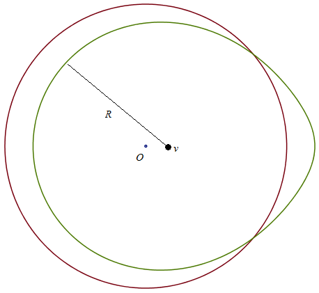 Figure 2
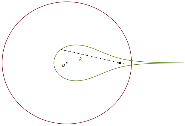 Figure 3
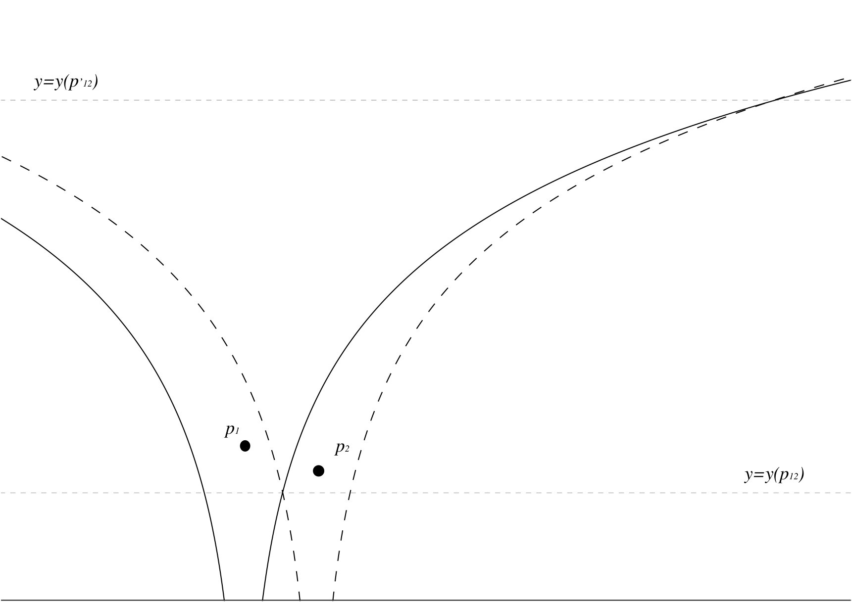 Figure 4
 Figure 5
 Figure 6
 Figure 7
 Figure 8
Peer Reviews
No public reviews on file for this paper yet. If you reviewed it on a platform where reviews are public (OpenReview, ICLR, NeurIPS, ICML), you can paste yours below so the community can read it here.
Videos
No videos yet. Explain this paper in a talk, walkthrough, or lecture? Add one.
Limit theory for isolated and extreme points in hyperbolic random geometric graphs
111 2010 Mathematics Subject Classification: Primary: 05C80 Secondary: 05C12, 05C82. Keywords: random geometric graphs, hyperbolic plane, complex networks, central limit theorem.
Nikolaos Fountoulakis222School of Mathematics, University of Birmingham, United Kingdom e-mail: [email protected]; Research partially supported by the Alan Turing Institute, grant EP/N510129/1 Joseph Yukich333Department of Mathematics, Lehigh University, USA e-mail: [email protected]; Research supported in part by Simons Collaboration grant 519427
(November 2, 2020)
Abstract
Given and , let be the disc of radius in the hyperbolic plane having curvature . Consider the Poisson point process having uniform intensity density on , with , and a fixed constant. The points are projected onto , preserving polar coordinates, yielding a Poisson point process on . The hyperbolic geometric graph on puts an edge between pairs of points of which are distant at most . This model has been used to express fundamental features of complex networks in terms of an underlying hyperbolic geometry.
For we establish expectation and variance asymptotics as well as asymptotic normality for the number of isolated and extreme points in as The limit theory and renormalization for the number of isolated points are highly sensitive on the curvature parameter. In particular, for , the variance is super-linear, for the variance is linear with a logarithmic correction, whereas for the variance is linear. The central limit theorem fails for but it holds for .
1 Introduction and main results
1.1 Hyperbolic random geometric graphs
We study in this paper the random geometric graph on the hyperbolic plane , as introduced by Krioukov et al. [16]. The standard Poincaré disk representation of is the open unit disk equipped with the hyperbolic (Riemannian) metric given by . Recall that the arclength of the boundary of a disk of radius and centered at the origin is , whereas the area of is .
Given a fixed constant and a natural number , we let
[TABLE]
i.e., . For every , consider the probability density function
[TABLE]
Let be uniformly distributed on . When the distribution of given by (1.1) is the uniform distribution on under the metric . For general Krioukov et al. [16] call this the quasi-uniform distribution on , since it arises as the projection of the uniform distribution on a disc of hyperbolic radius in , the hyperbolic plane having curvature and equipped with the metric .
Denote by the Borel measure on given by
[TABLE]
where is a Borel subset of . We let denote the Poisson point process on with intensity measure . Denote by the probability space on which the point process is realised. Let denote expectation with respect to .
We join two points in with an edge if and only if they are within hyperbolic distance of each other. The resulting hyperbolic random geometric graph on is denoted by . Figure 1 illustrates the disc of radius centered at .
An equivalent construction of goes as follows. Given and , let be a disc of radius in . Consider the Poisson point process having uniform intensity density on . The points are projected onto , preserving polar coordinates, and the hyperbolic geometric graph on is created by putting an edge between the points of the Poisson point process whose projections are distant at most . The projection of this graph onto is .
When is replaced by i.i.d. random variables having density , we obtain the model of Krioukov et al. [16]. The underlying hyperbolic geometry gives rise to a power-law degree distribution tuned by the parameter , whereas the parameter determines the average degree of [16]. The model realises the assumption that there are intrinsic hierarchies in a complex network that induce a tree-like structure. This set-up provides a geometric framework describing the inherent inhomogeneity of complex networks and suggests that the geometry of complex networks is hyperbolic.
The graph also arises as a cosmological model. As noted in [15], the higher-dimensional analogue of asymptotically coincides as with the graph encoding the large scale causal structure of the de Sitter spacetime representation of the universe. Roughly speaking, the latter graph is obtained by sprinkling Poisson points in de Sitter spacetime (the hyperboloid) and then joining two points if they lie within each other’s light cones. The light cones are then mapped to the hyperbolic plane, where they are approximated (for large times) by the hyperbolic balls of a certain radius (see Fig. 2 in [15]). Graph properties of thus yield information about the causal structure of de Sitter spacetime.
1.2 Main results
For any we let denote its radius (hyperbolic distance to the origin) and
[TABLE]
its defect radius. Given a point process on and , we say that is isolated with respect to if and only if there is no , , such that . We say that is extreme with respect to if and only if there is no , , such that and
Given , define the score to be if is isolated with respect to and zero otherwise. Likewise, define to be if is extreme with respect to and zero otherwise. Our main goal is to establish the limit theory for the number of isolated and extreme points in , given respectively by
[TABLE]
and
[TABLE]
Isolated vertices are well-studied in the setting of Euclidean graphs, where they feature in the connectivity properties of certain random graph models. The paper [22] elaborates on this when the graph in question is either the geometric graph on i.i.d. points in or even a soft version of this graph. In the cosmological set-up [15], in the large time limit, isolated points are precisely those whose past and future light cones are empty, i.e., the set of points neither accessible by the past nor having access to the future. Extreme points are those whose future light cones are empty, i.e., points which do not causally influence other points.
Extreme points are the analog of maximal points of a sample, of broad interest in computational geometry, networks, and analysis of linear programming. Recall that if is a cone with apex at the origin of , then given locally finite, is -maximal if . If is an i.i.d. sample uniformly distributed on a smooth convex body in of volume , , then both the expectation and variance of the number of maximal points in are asymptotically , the order of the expected number of points close to the boundary of [25]. In the present paper, the expectation and variance of the number of extreme points are shown to grow linearly with , which likewise is of the order of the expected number of points close to the boundary of .
The second order limit theory for the number of isolated points is altogether different. Our first main result shows that the growth rates of the variance of decrease with increasing and undergo a double jump when crosses . Moreover, there is a logarithmic correction at . The variance grows faster than the expectation for , but it is always sub-quadratic with respect to input size. The asymptotics for the range contrast markedly with the second order limit behavior of isolated points in the random geometric graph in the Euclidean plane [21], where asymptotics grow linearly with input. This phenomenon, which gives rise to non-standard renormalization growth rates, appears to be linked to the high connectivity properties of for small , as described in Section 1.3.
The limit constants appearing in our first and second order results (1.3), (1.5), and (1.6) are given in terms of expectations and covariances of scores involving isolated and extreme points of a Poisson point process on the upper half-plane, which appears to be a natural setting for studying such problems. Put .
Theorem 1.1**.**
We have for all
[TABLE]
and
[TABLE]
On the other hand, for all , the expectation and variance asymptotics for the number of extreme points exhibit linear scaling in , that is to say the renormalization is the standard one in stochastic geometric models.
Theorem 1.2**.**
We have for all
[TABLE]
and
[TABLE]
where are given by (5.2) and (5.10), respectively, below.
Denote by the standard normal random variable with mean zero and variance one. One might expect that , after centering and renormalizing, converges in distribution to for all . The next result shows that this is false.
Theorem 1.3**.**
As , for any we have
[TABLE]
The limit (1.7) fails for . As , for any we have
[TABLE]
The proofs of these results depend on mapping the point process in the disc to a Poisson point process hosted by a rectangle in the upper half-plane. This mapping, introduced in [9], transforms the graph into an analytically more tractable graph, as seen in Section 2. In particular, it facilitates the evaluation of the probability content of the intersection of two radius balls, which is essential to evaluating the covariance of scores at distinct points. Variance calculations are based on the covariance formula for two points. In the case of isolated points, the upper bound is based on the Poincaré inequality. The lower bound, which turns out to be tight, is based on a careful analysis of the intersection of the balls of radius around two typical points. We refer the reader to Sections 3 and 4 for all details.
The determination of variance asymptotics for is handled by extending stabilization methods. That is, for a given point , we define a radius of stabilization for , in the sense that points at distance farther than from do not affect the property of being extreme. We show that the covariance of two points (depending on their interpoint distance and heights) is rather small. By stabilization, the covariance converges to the covariance of two points in the infinite hyperbolic plane. We show in Section 5 that though the constants describing the tail behavior of grow exponentially fast with the height of , it is still possible to extract an explicit integral formula for the scaled variance.
To prove the asymptotic normality (1.7) we use the Poincaré inequality for Poisson functionals [17], which bounds the Wasserstein distance in terms of first- and second-order difference operators. When there is a high probability event on which these difference operators may be controlled, as vertices of high degree are fewer in this regime. For , conditional under the likely event of having no vertex sufficiently close to the origin (equivalently having no vertex of significantly high degree), the variance is much smaller than the unconditional variance, and the convergence to the standard normal fails in this regime. Intuitively, vertices close to the origin generate radius balls which cover a relatively large part of and any vertex lying therein will not be isolated. Surprisingly, when , this phenomenon stops having a significant effect and, therefore one can deduce the asymptotic normality of .
The case of extreme points is different, since the extremality status of a point is influenced only by points of larger radius lying in the ball of radius around it. This region is typically quite small and makes the corresponding score functions almost independent. To prove the central limit theorem (1.8), we cut the plane into rectangles and define a dependency graph on the vertex set of such rectangles, so that no points in non-adjacent vertices in this dependency graph can be connected, and we use the central limit theorem of Baldi and Rinott [3].
Remarks. (i) We are unaware of results treating the limit theory for statistics of in the regime The paper [24] establishes variance asymptotics and asymptotic normality for the number of copies of trees in with at least two vertices, but the authors require , save for when counting trees close to the boundary of . The methods of [24] do not appear to treat the limit theory of and , as .
(ii) It is an interesting problem whether the number of isolated points asymptotically follows a normal law when . The methods in this paper do not apply, as they give estimates that are useless. To deal with this case, one likely needs a more detailed treatment of the variance of , giving not only the order of magnitude but the multiplicative constant.
(iii) As seen in [5, 10], the expected number of cliques of order is if , whereas the expected number of cliques of order is if
(iv) In dimension we expect that the central limit theorem (1.8) holds for all , where is suitably defined so that the average degree of the random graph is . It is unclear for which the central limit (1.7) holds in dimension .
(v) It is unclear whether there exists a limiting distribution for when . As we are going to see in Section 6, the variance of is highly sensitive when conditioning on the high probability event of having no points within a certain radius in . It is plausible that a central limit theorem holds in such a conditional space.
(vi) As elaborated upon in the next subsection, the degree distribution in follows a power-law with exponent when . In particular, the degree distribution belongs to when . It would be worthwhile to better understand the connection between asymptotic normality of the number of isolated vertices and moments of the degree distribution.
Notation and terminology. We say that a sequence of events occur asymptotically almost surely (a.a.s.) if . Given and two sequences of positive real numbers, we write to denote that , as .
1.3 Degree and connectivity properties of the graph
For , the tails of the distribution of the degrees in follow a power law with exponent ; see Krioukov et al. [16]. This was verified rigorously in [12]. For , the exponent is between 2 and 3, as is the case in a number of networks arising in applications (see for example [2] for a list of experimental observations). The paper [16] observes that the average degree of is determined through the parameter for . This was rigorously shown in [12]. In particular, they show that the average degree tends to in probability. However, when , the average degree tends to infinity as . Thus, in this sense, the regime corresponds to the thermodynamic regime in the context of random geometric graphs on the Euclidean plane [21]. In [8] the degree distribution of a soft version of this model is determined. Here, pairs of points that are distant at most are joined with some probability that is not identically equal to 1.
When is small, one expects more points of to be near the origin and one may expect increased graph connectivity. The paper [6] establishes that is the critical point for the emergence of a giant component in . In particular, when , the fraction of the vertices contained in the largest component is bounded away from 0 a.a.s. [6], whereas if , the largest component is sublinear in a.a.s. For , the component structure depends on . If is large enough, then a giant component exists a.a.s., but if is small enough, then a.a.s. all components have sublinear size [6]. Figures 2 and 3 illustrate these transitions.
The paper [9] strengthens these results and shows the fraction of vertices belonging to the largest component converges in probability to a constant which depends on and . Furthermore, for , there exists a critical value such that when crosses a giant component emerges a.a.s. [9]. For the second largest component has polylogarithmic order a.a.s.; see [13] and [14]. For we have that is a.a.s. connected, whereas is disconnected for [7]. For , the probability of connectivity tends to a certain constant given explicitly in [7].
Apart from the component structure, the geometry of this model has been also considered. In [13] and [11] polylogarithmic upper bounds on the diameter are shown. These were improved shortly afterwards in [19] where a logarithmic upper bound on the diameter is established. Furthermore, in [1] it is shown that for the largest component has doubly logarithmic typical distances and it forms what is called an ultra-small world.
2 Auxiliary results
2.1 Approximating a hyperbolic ball
We characterize when two points in are within hyperbolic distance . In particular the next lemma approximates hyperbolic balls by analytically more tractable sets, reducing a statement about hyperbolic distances between two points to a statement about their relative angle. For a point , we let be the angle between and a (fixed) reference point (where positive angle is determined by moving from to in the anti-clockwise direction). For points we denote by their relative angle:
[TABLE]
For any recall that denotes its radius (hyperbolic distance to the origin) whereas , or more succinctly . Thus for , we shall write . The hyperbolic law of cosines relates the relative angle between two points with their hyperbolic distance:
[TABLE]
For , we let be the value of satisfying (2.1), having set , for two points with and . As is decreasing in , it follows that if and only if .
When and are not too large, our next result estimates as a function of and . To prepare for mapping to a rectangle in having length proportional to , we re-scale by a factor of . The following lemma appears in a stronger form in [9]. Here and elsewhere we put
[TABLE]
The proof of the next lemma is in Section A.
Lemma 2.1**.**
Given and in , , and , with we set
[TABLE]
For every there exists a such that the following holds.
- (i)
If , i.e., if , then
[TABLE] 2. (ii)
If , i.e., if , then
[TABLE]
where as , uniformly over all . 3. (iii)
In part (i) above, one can take and as . In particular we may relate and by .
Recall that denotes the disc of (hyperbolic) radius centered at the origin . For any we let denote the annulus . Throughout we shall use caligraphic letters to denote subsets of . For we let . We now approximate whenever , with as in Lemma 2.1. This goes as follows.
By the triangle inequality, given , any point with defect radius at most is also within distance from . To approximate from above, we will take a superset of this set, namely the set of points of radius at most , with as in Lemma 2.1. We set and and put
[TABLE]
and
[TABLE]
For , as in Lemma 2.1(i), and with , the inequality (2.3) yields the following inclusions:
[TABLE]
In our calculations for we will need the truncated subset of consisting of points with height coordinates at most , namely
[TABLE]
A point is extreme with respect to if and only if . Lemma 2.1(ii) implies that if , then
[TABLE]
2.2 Properties of
The density of the defect radius is close to the exponential density with parameter . The proof of this fact is based on elementary algebraic manipulations and appears in Section A.
Lemma 2.2**.**
Let be the probability density of the defect radii. For all we have
[TABLE]
One does not expect to observe isolated and extreme points close to the origin. The following lemma makes this precise and shows that the isolated and extreme points a.a.s. have defect radii less than .
Lemma 2.3**.**
Let . If then for all we have
[TABLE]
Proof.
Let and be as in Lemma 2.1. First assume that . We may bound by the probability that is empty. Using the first inclusion in (2.5) and recalling the definition of at (1.2), we have (for sufficiently large):
[TABLE]
where the inequality follows by Lemma 2.2.
Suppose now that , i.e, . By the triangle inequality any point of of radius less than is within hyperbolic distance from . This implies that
[TABLE]
Recalling (1.2) we obtain
[TABLE]
whereby
These upper bounds are also valid for , with the exception of the last integral which would start from instead of from . However, the asymptotic growth of this integral is still . ∎
2.3 Mapping to
To further simplify our calculations, we will transfer our analysis from to , making use of a mapping introduced in [9]. We set
[TABLE]
For any subset , define the rectangular domain
[TABLE]
and we put
[TABLE]
For , recall that we write , with the defect radius and the angle with respect to a reference point. We re-scale the angle by , setting . This defines the map , mapping .
Put . The map sends to the Poisson point process on with intensity density
[TABLE]
where, recalling Lemma 2.2, we have , since .
The analogue of the relative angle is defined as follows. For , we let
[TABLE]
When considering the geometry of hyperbolic balls inside , it will be convenient to use arithmetic on the -axis modulo . In particular, for , we write , if and or and . This definition naturally extends to all other types of inequalities. Also, for any , we write , if .
Mapping balls in to balls in . We set
[TABLE]
Thus, for with and , we have
[TABLE]
and
[TABLE]
For with note that transforms the set inclusion (2.5) into
[TABLE]
Approximating and on . Let be the image of by . For we define . In other words,
[TABLE]
Regarding , recall from (2.7) that is extreme if and only if . The image under of the truncated ball at (2.6) is
[TABLE]
Note that if and only if For define
[TABLE]
By definition, we thus have and
[TABLE]
From now on, when the context is clear, we write instead of for a generic point in .
Lemma 2.4**.**
We have for all
[TABLE]
and similarly when is replaced by .
Proof. This follows from Lemma 2.3. ∎
We put
[TABLE]
and
[TABLE]
Lemma 2.5**.**
We have for all
[TABLE]
as well as
[TABLE]
Proof.
For brevity we write for and for . We first assert that
[TABLE]
To see this, we condition on the event that (note that the complementary event has probability which is generously bounded by ) and then use Boole’s inequality together with Lemma 2.4.
Now write
[TABLE]
By Hölder’s inequality and (2.14), we have
[TABLE]
[TABLE]
Using the inequality , together with , we see that which proves the first assertion in Lemma 2.5. The remaining assertions are proved similarly. ∎
Define the Poisson point process on with intensity measure given by
[TABLE]
where is measurable. Recall from (2.9) that Put
[TABLE]
and
[TABLE]
The following lemma, together with Lemma 2.5, shows that to prove Theorems 1.1 and 1.2, it is enough to establish expectation and variance asymptotics for and .
Lemma 2.6**.**
We have for all
[TABLE]
and
[TABLE]
We will show that and are both . This, together with the following corollary of Lemmas 2.5 and 2.6, implies that the leading terms of and are given by and , respectively.
Corollary 2.7**.**
We have for all
[TABLE]
and
[TABLE]
Proof of Lemma 2.6. Let be and let be . We denote by the event that . By Lemma 2.2, there is a coupling of the point processes and such that , since . We let and . Then . Setting and gives
[TABLE]
Now,
[TABLE]
since is Poisson-distributed with parameter equal to . Thus The bound remains valid if we interchange with , with , and with . We thus obtain The proof of the bound for is identical, except that second moments are replaced by first moments and this yields . This completes the proof of the estimates involving and . The proofs of the assertions involving and are identical. ∎
3 Preparing for the proof of Theorem 1.1
We provide several lemmas needed to estimate .
3.1 A covariance formula for
We establish a basic covariance formula needed for the calculation of . If is a score function, we define the covariance of at the points as
[TABLE]
We will give an expression for . The number of points of inside is Poisson-distributed with parameter , implying that Thus
[TABLE]
Put
[TABLE]
If and , then we have
[TABLE]
Therefore, given , we have the following basic covariance formula:
[TABLE]
Consider the second case in (3.3), where the covariance is negative. By Lemma 2.1(ii), given points and with , we have
[TABLE]
where uniformly for all . Setting
[TABLE]
we may re-state the above as
[TABLE]
Before focussing on the first case in (3.3) we need some geometric preliminaries.
3.2 The geometry of balls with height coordinate at most
Our aim now is to estimate . The set inclusion at (2.11) implies
[TABLE]
Given , and we set
[TABLE]
[TABLE]
and
[TABLE]
We continue to assume that and belong to . We assume without loss of generality that and . Henceforth, for as in Lemma 2.1, we put
[TABLE]
Notice that and . See Figure 5.
Furthermore, the definitions of and and the assumption imply
[TABLE]
and
[TABLE]
These inclusions yield
[TABLE]
and
[TABLE]
whence
[TABLE]
First, we notice that the definitions of and give
[TABLE]
Denote by either of the balls or and denote by either or , depending on which of the two cases we are considering. The following lemma characterises when two balls are disjoint.
Lemma 3.1**.**
Fix and assume . With at (3.9) we have if and only if
[TABLE]
Proof.
By the definition of , the right-most point of , denoted by satisfies . Similarly, the left-most point of (denoted by ) satisfies . Note that . Then if and only if . If , then . Likewise, if , then . ∎
We still assume and we set . With at (3.9) we consider in the remainder of this sub-section the case . For in this domain, Lemma 3.1 implies that . Given , denote the left and right boundaries of by
[TABLE]
and
[TABLE]
cf. Figure 5. The first part of the next lemma shows that and intersect whenever the -coordinates of and are far enough apart with respect to the exponentiated height coordinates.
Lemma 3.2**.**
(i) If then
[TABLE]
(ii) . (iii) If then
[TABLE]
Proof. (i) If (cf. Figure 6), then satisfies the following equations:
[TABLE]
Therefore
[TABLE]
Hence, exists provided that , which implies (3.14), as desired.
(ii) On the contrary, assume that there exists . Using the definition of the left boundary we have
[TABLE]
We deduce that
[TABLE]
since , which is impossible. Thus, such cannot exist and , proving (ii) as desired.
(iii) Assume (cf. Figure 6). Then satisfies
[TABLE]
which yields (3.15) and completes the proof of Lemma 3.2. ∎
Note that (3.15) and (3.16) imply that . For convenience, we will set
[TABLE]
Consider now the union of the two balls . For any let and be such that . Then . Now for , consider two points and such that . Since , it follows that . In other words, the curves and do not intersect and stays “above” .
3.3 The -content of
We now focus on and . The calculations of the -measure of these two intersections are similar, as the considered sets differ only by constant factors and . We provide a generic calculation covering both cases. The inequality (3.12) shows that the -content of
[TABLE]
controls the growth of . The following lemma gives quantitative bounds on . We will use the first part of the lemma to lower bound . It turns out that this gives the main contribution to the variance bound of Theorem 1.1. We will give a matching upper bound on the variance through the Poincaré inequality. The second part of the lemma gives an upper bound on the intensity measure of , which will be used in the proof of the central limit theorem for . Recall from (3.9) that we have set Also, recall that we set .
Lemma 3.3**.**
Let , as above. For we put , we set , and we suppose that .
- (i)
If , then
[TABLE]
where
[TABLE] 2. (ii)
If , then
[TABLE]
Proof.
Part (i). We express as the disjoint union of the sets and . The above analysis implies that . Let us consider the region . Let . Then any point with belongs to if and only if . Note that .
Recalling , these observations imply
[TABLE]
We also have
[TABLE]
Hence, by (3.20) and (3.21) we have
[TABLE]
[TABLE]
Therefore,
[TABLE]
Combining (3.23) and (3.24) yields
[TABLE]
Substituting (3.24) and (3.25) into (3.22) we have
[TABLE]
Notice that
[TABLE]
Substituting this into (3.26) yields
[TABLE]
Hence, the proof of part (i) is complete.
Part (ii). We will consider three different subsets of the interval . For the case where we will use part (i). (Note that , since .) Indeed, the expression for immediately implies that for any such we have
[TABLE]
Now, assume that . In this case, we have . Thus, any point with and belongs to if and only if . Hence, we will use a modified version of (3.21):
[TABLE]
Using (3.24) and (3.25), the above becomes:
[TABLE]
(Note that when , the above expression is equal to 0.) Now, since we obtain
[TABLE]
Recalling that we deduce that . So
[TABLE]
which yields (3.19) when satisfies .
Finally, assume that . By Lemma 3.1 we have that and therefore
[TABLE]
Since , the above expression is , which also yields (3.19). Combining the three cases together we deduce part (ii). ∎
4 Proof of Theorem 1.1
A central tool in the proof of our main results is the Palm theory for Poisson processes (see [21, 23, 18]). Let be a measurable space and the set of all locally finite point configurations on . For a Poisson point process on with intensity and a measurable non-negative function the Campbell-Mecke formula (cf. Theorems 4.1, 4.4 of [18]) gives
[TABLE]
where the sum ranges over all pairwise distinct -tuples of points of .
Equation (4.1) can be used to calculate where for some score function on taking values in . With (cf. (3.1)), the definition of the variance together with (4.1) yield:
[TABLE]
where the last equality holds since (in fact the first equality does not require that the score function is an indicator random variable, but this is the case throughout our paper).
4.1 Proof of expectation asymptotics (1.3)
Lemma 4.1**.**
Uniformly for we have
[TABLE]
Proof. We use the inclusions in (2.11). By Lemma 2.1(iii) we may put and . Now (2.11) yields:
[TABLE]
where we recall that and where and are related via . Recalling , , and , it follows that uniformly over all such
[TABLE]
We conclude that (Recall that and .) Notice that since . Thus , uniformly over all such , whereby
[TABLE]
To obtain a lower bound, we use the first inclusion in (2.11):
[TABLE]
Using again that and we deduce a matching lower bound:
[TABLE]
Combining (4.5) with (4.6) shows (4.3), as desired. ∎
We now establish expectation asymptotics (1.3). Since
[TABLE]
it follows from (4.3) that
[TABLE]
uniformly over all . The Campbell-Mecke formula (4.1) and (4.7) yield
[TABLE]
since . By Lemmas 2.5 and 2.6, we deduce (1.3) as desired. ∎
4.2 Upperbounding
We derive the asymptotics for in two steps. First, in this subsection we provide an upper bound via the Poincaré inequality. It turns out that this is tight up to multiplicative constants. The next subsection provides a matching lower bound for using the geometry of the intersection of hyperbolic balls obtained in Section 3.
Let be a functional on a space hosting a Poisson process of intensity measure . For a point we define the first order linear operator . Then the Poincaré inequality (inequality (1.1) in [17]) states that
[TABLE]
We now put
[TABLE]
Note that is stochastically dominated from above by the number of points of in . By Lemma 4.1 we deduce that is Poisson-distributed with parameter equal to
[TABLE]
uniformly over all , for some constant . Thus,
[TABLE]
which implies that
[TABLE]
In other words, evaluating the integral and using in the range , we get
[TABLE]
4.3 Lowerbounding
Recall the definition of at (3.1). By (4), we have with
[TABLE]
and
[TABLE]
Since it suffices to provide a lower bound on matching that at (4.9). Put
[TABLE]
where , , and . By symmetry, it suffices to consider the case where and . Indeed, this is one of four possible cases regarding the relative positions of and it accounts for the pre-factor 4 appearing in front of our upcoming lower bounds.
Note that if and , then in fact . Considering points and such that , , and we have by (3.3) the bound
Therefore,
[TABLE]
We will drop the sign and write Note that does not depend on as the Poisson process is stationary with respect to the spatial -coordinate. Therefore, we can write
[TABLE]
We change variables and, as before, put . Hence, and . Also, . Moreover, as ranges from [math] to , the variable ranges from to . Thus,
[TABLE]
To simplify notation we shall write
[TABLE]
This amounts to transferring the term inside changing the constant to . It will make no difference.
Let us observe that
[TABLE]
where, recalling defined at (3.4), we have
[TABLE]
By (3.5) the covariance is negative only when belongs to the range covered by the integral. For , the covariance is positive. Thus, for the range it suffices to use the subset given by the smaller range of which in turn is covered by Lemma 3.3(i).
For we set
[TABLE]
We now show that for all , whereas we derive lower bounds on which match the upper bounds in (4.9).
4.3.1 Calculating integral
Formula (4.7) and the second part of the covariance formula (3.3) give for all
[TABLE]
uniformly for all , whereby
[TABLE]
Therefore, since by (3.4), we eventually obtain:
[TABLE]
Hence, we deduce for all that
4.3.2 The lower bound on integral
Let and . Given the domain consider the sub-domain
[TABLE]
It suffices to consider the contribution to that comes from the domain . That is, we will bound from below the integral
[TABLE]
Combining (3.3), Lemma 3.3, (4.7) and recalling we obtain
[TABLE]
For simplicity, we set and , whereby
[TABLE]
Consider the integral in (4.14) when . The following lemma shows that its value changes radically as crosses 1. The regimes for this lemma induce three regimes for .
Lemma 4.2**.**
There is a such that for any sufficiently large, any and , we have
[TABLE]
Proof. Elementary integration gives the three different cases:
[TABLE]
By definition, for any , we have that , whereas , for sufficiently large. Thus, as . These facts imply that if , then for some
[TABLE]
whereas if , then
[TABLE]
Finally if , then , for sufficiently large. The lemma follows. ∎
For and sufficiently large we have . In this domain the definition of gives
[TABLE]
4.3.3 Three regimes for integral
4.3.3 (a) The integral , . Recalling the definitions of and and appealing to Lemma 4.2, we deduce the following lower bound
[TABLE]
Recall from (3.18) that . For any sufficiently small (in terms of ), we have . Therefore,
[TABLE]
We then deduce that
[TABLE]
Recall that . This implies that
[TABLE]
The above bounds imply that
[TABLE]
Thus, for we have
[TABLE]
4.3.3 (b) The integral , . Note first that
[TABLE]
In this case, the integral in (4.14) is bounded below as follows:
[TABLE]
where the last inequality holds for sufficiently large, if we put (cf. Lemma 2.1(iii)). In particular, if we let , then
[TABLE]
Also, recall that . Since , it follows that for sufficiently large we have . Combining this observation with the above lower bound, (4.14) yields
[TABLE]
Therefore
[TABLE]
4.3.3 (c) The integral , Recall by (4.15) that for any , we have
[TABLE]
for some . Since when is sufficiently large, we get
[TABLE]
Using the third case in Lemma 4.2, the integral in (4.14) is bounded from below as follows:
[TABLE]
Hence,
[TABLE]
4.4 Proof of growth rates for
We have now estimated the two summands that bound the main term of from below. Our findings are summarised as follows:
[TABLE]
By (4.10) we have and . Therefore,
[TABLE]
As , we finally deduce that
[TABLE]
Combining (4.9) and (4.21), and recalling Corollary 2.7, we thus establish the desired growth rates for , completing the proof of (1.4).
5 Proof of Theorem 1.2
5.1 Proof of expectation asymptotics for
By Lemmas 2.5 and 2.6 it suffices to compute . Given a point we have
[TABLE]
Similarly, we have the lower bound
[TABLE]
Taking again , and , we then deduce that uniformly over all
[TABLE]
Therefore,
[TABLE]
uniformly over all . Hence, the Campbell-Mecke formula (4.1) yields
[TABLE]
as desired.
5.2 Proof of variance asymptotics for
The determination of variance asymptotics for is handled by extending existing stabilization methods. We show that when the constants describing the tail behavior of the stabilization radius at a point are allowed to grow exponentially fast with the height of , as at (5.5) below, then one may nonetheless establish explicit variance asymptotics as , as shown in the analysis between (5.12) and (5.14) below.
We first require several auxiliary lemmas. For all and we let denote the closed Euclidean ball of radius centered at .
The identity (2.6) implies that for we have
[TABLE]
We set , where .
Put . We let be the Euclidean distance between and the point in which is closest to . Set and note . Now we put
[TABLE]
The extremality status of depends only on the point set in the sense that points outside this set will not modify . In other words,
[TABLE]
that is to say that is a radius of stabilization for .
Clearly, for , we have . We seek to control , as a function of both and the height parameter . Put and set for . We assert there is a constant such that for we have
[TABLE]
We first compute lower bounds on the probability content of the regions
[TABLE]
Lemma 5.1**.**
Let . For all large we have
[TABLE]
Proof. First assume Notice that meets the positive -axis at points which have absolute value exceeding when . In other words, we have . We also have , implying . Consequently, we have
[TABLE]
Now assume Since exceeds , we have . As above, it follows that
[TABLE]
Hence
[TABLE]
where the last inequality uses . Hence, as desired. ∎
Now we note that iff which happens if . Lemma 5.1 shows that for
[TABLE]
For we have the trivial bound
[TABLE]
Put for . Summarizing the above we have shown for that
[TABLE]
It remains to show that (5.4) holds for . Recall that the left-hand side of (5.4) vanishes for in the range . If and then . For large enough we thus have
[TABLE]
Thus we have shown (5.3) as desired.
Recall that . Since is stationary with respect to the spatial -coordinate it follows that for all , we have
[TABLE]
Given the bound (5.6), we now find asymptotics for . In the remainder of this section we continue to abbreviate by . In the next lemma, we will bound the covariance of with respect to , namely
[TABLE]
Lemma 5.2**.**
There is a constant such that for all , we have
[TABLE]
Proof. Write . Put and define . Since is bounded by , we note that
[TABLE]
differs from
[TABLE]
by at most .
Notice that
[TABLE]
We consequently obtain
[TABLE]
By independence we have
[TABLE]
Likewise
[TABLE]
differs from
[TABLE]
by at most . We conclude that
[TABLE]
The bound (5.3) completes the proof. ∎
Recall that is the Poisson point process on with intensity measure as at (2.15). Next, define analogously as in the definition of . Note that as . The next lemma follows from stabilization methods; see for example [4], [20].
Lemma 5.3**.**
We have
[TABLE]
Now we may finally prove the asserted variance asymptotics at (1.6). Put
[TABLE]
By (2.19), it is enough to show that
[TABLE]
*Proof of (1.6). * We have by (4)
[TABLE]
The first integral in (5.12) reduces to by translation invariance of in the spatial coordinate. The stabilization of shows for all that
[TABLE]
By the dominated convergence theorem and using and , we obtain
[TABLE]
[TABLE]
Now we turn to the second integral in (5.12). By translation invariance in the spatial coordinate we have
[TABLE]
[TABLE]
[TABLE]
Let , . Then since the above becomes
[TABLE]
For every we have by (5.7) that is dominated by an integrable function of . It follows by the dominated convergence theorem that for every we have
[TABLE]
[TABLE]
The second integral in (5.12) thus converges to
[TABLE]
Notice that is the sum of (5.13) and (5.14). This completes the proof of Theorem 1.2. ∎
6 Proof of Theorem 1.3
To prove (1.7) and (1.8), we first assert that it suffices to prove central limit theorems for the random variables and , defined at (2.16) and (2.17), respectively. We prove this assertion for as the proof for is identical.
Set to be . Recall that is determined by the Poisson process on defined at (2.10) whereas is determined by defined at (2.16). By Lemma 2.2, the intensities of these two processes differ by . We can couple these two processes using a sprinkling argument. Let be the Poisson process on with intensity equal to at - in other words the minimum of the intensities of and . Now, we define two other independent processes on : of intensity at and of intensity at . The union of and is distributed as , whereas the union of and is distributed as . We will use the symbols and to denote the copies of these processes in the coupling space. For each , we may define the coupling space to be the product of the spaces on which , , and are all defined. Let denote the product probability measure on the coupling space.
Thus, for any
[TABLE]
This implies that on the coupling space we have with probability as . Also, the coupling will allow us to assume that and are defined on the same probability space.
Furthermore, by Lemmas 2.5 and 2.6 we have
[TABLE]
In particular, the former implies that . Henceforth, if , is a sequence of random variables with defined on the coupling space, then by we mean that for all we have as .
Thus we have as , whence
[TABLE]
as well. If , and are sequences of random variables with , if , and if , is a sequence of scalars with , then . Since it follows that as we have
[TABLE]
Thus the asymptotic normality for implies the asymptotic normality of , i.e., we have as
[TABLE]
In the following sub-sections, we will show that and satisfy a central limit theorem, the former for all and the latter for all . These imply (1.7) and (1.8). On the other hand, in the final sub-section, we show that does not satisfy a central limit theorem for . The above argument implies that also does not satisfy a central limit theorem in the same range of .
6.1 The central limit theorem for
Consider the ball centered at a point . We compute the maximum -distance between and a generic point in the intersection of . This tells us the maximum -distance of the set given by the intersection of with . Since both and have heights at most , the inclusion at (2.11) implies that
[TABLE]
We define a dependency graph as follows. Firstly, we partition the interval into consecutive intervals of equal length, which we enumerate . For each , we set . The collection of axis-parallel rectangles partitions . The vertex set consists of the rectangles . We put an edge between any two rectangles whenever and are separated by a rectangle having -distance at most . Let be the collection of all such edges. Put for all
[TABLE]
By the definition of , if and are disjoint collections of rectangles in such that no edge in has one endpoint in and the other endpoint in , then the random variables and are independent. Note that a rectangle having -side equal to will have non-empty intersection with at most
[TABLE]
rectangles from the collection .
Thus is a dependency graph for Now note that
[TABLE]
Furthermore,
[TABLE]
Standard tail estimates for Poisson random variables give , for sufficiently large. So
[TABLE]
Define
[TABLE]
The maximal degree of the dependency graph satisfies We also set , . Set . Hölder’s inequality gives
[TABLE]
and
[TABLE]
We thus conclude that
[TABLE]
and
[TABLE]
We have shown that and thus also . The Baldi-Rinott central limit theorem for dependency graphs [3] gives
[TABLE]
Since , we have . This shows a central limit theorem for conditional on .
To deduce a central limit theorem for , we write
[TABLE]
Since conditional on satisfies a central limit theorem by (6.6), the probability on the right-hand side converges to . ∎
6.2 The central limit theorem for : the regime
The above approach turns out to be not strong enough for showing the asymptotic normality for the number of isolated vertices. For a certain range of a dependency graph defined as above has high maximum degree making the bounds (6.6) of little use. We will instead prove a central limit theorem for using a Poincaré-type inequality for Poisson functionals due to Last, Peccati and Schulte [17].
Let denote a Poisson point process on a space having intensity measure . Let denote a functional on locally finite point sets in . Recall that for a point we defined the first order linear operator . Here, we will also use the second order operator . The functional belongs to the domain of if
[TABLE]
Theorem 1.1 of [17] uses these differential operators to approximate the normalised version of by the standard normal . For two real-valued random variables and , let denote the Wasserstein distance between the measures on induced by and .
Theorem 6.1**.**
Let be a functional defined on locally finite collections of points in . Assume belongs to the domain of and satisfies and . If is a standard normally distributed random variable, then
[TABLE]
where
[TABLE]
We will apply Theorem 6.1 on the conditional space of the event
[TABLE]
A calculation similar to the one in (6.2) shows that for any we have
We shall apply Theorem 6.1 setting to be and letting
[TABLE]
These ensure that on , one has and . We will verify that is on the domain of later on, using the estimate on . We will only check the second condition; the requirement that follows from our bounds on .
Set and . The proof of the next lemma is postponed until Section B.
Lemma 6.2**.**
For any , we have
[TABLE]
To apply Theorem 6.1 we shall bound by the number of points of which are inside the hyperbolic ball around having height at most . By the inclusion-exclusion principle, the second order operator is proportional to the number of isolated points of which are contained in the intersection of the hyperbolic balls around and and having height at most . Thus
[TABLE]
Given a Borel-measurable set , we have that is a Poisson-distributed random variable with parameter equal to the intensity measure of . The next lemma, a consequence of Lemma 4.1, bounds these intensity measures for the sets appearing in (6.8).
Lemma 6.3**.**
There exists a constant depending on and such that for all we have
[TABLE]
*Hence, *
[TABLE]
Set . Thus, is stochastically dominated from above by a random variable , where distributed as . Analogously, is stochastically dominated by a Poisson-distributed random variable with parameter . We now bound , and in this order.
Lemma 6.4**.**
If , then .
Proof. For ,
[TABLE]
We deduce that
[TABLE]
Recall that and by the first part of Lemma 6.2 and (4.21). Therefore if then
[TABLE]
If , then ∎
Let us point out that the bound on is also a bound on and thus is in the domain of .
Lemma 6.5**.**
If , then .
Proof. The second inequality in (6.8) implies
[TABLE]
Now, we claim that there exists a constant such that if
[TABLE]
then . Indeed, for any we have where is defined at (3.7). Now, Lemma 3.1 implies that there exist some constant such that if (6.9) holds. This implies that when we integrate with respect to and , relative distances with respect to greater than this quantity have no contribution to the integral defining . In other words, (and , respectively) contributes to this integral only if
[TABLE]
Therefore, when we integrate over the choices of against the intensity measure (letting and ), we will get (using that )
[TABLE]
By the Cauchy-Schwarz inequality we have
[TABLE]
Using this inequality and integrating first with respect to and we obtain
[TABLE]
To bound the triple integral in (6.11) for , we will split the domain of integration into four sub-domains:
[TABLE]
We evaluate the integral in (6.11) on each of these four sub-domains. On we have:
[TABLE]
For the second sub-domain , we get:
[TABLE]
The third sub-domain gives an identical result due to symmetry.
Finally, for the fourth sub-domain we get:
[TABLE]
Combining the integrals for each of the four sub-domains we obtain
[TABLE]
Substituting the bound (6.12) into (6.11) we deduce for that This completes the proof of Lemma 6.5. ∎
Lemma 6.6**.**
If , then .
The proof of this lemma is almost identical to the proof of the previous lemma. We postpone it to Section C.
We now establish the central limit theorem at (1.7). Consider the random variable
[TABLE]
on the conditional space . Theorem 6.1 and Lemmas 6.4- 6.6 yield
[TABLE]
Recalling that , we have
[TABLE]
where the last equality follows by Lemma 6.2. Since the bound (6.13) shows that satisfies a central limit theorem on , the probability on the left-hand side of the above display converges to . Thus the central limit theorem (1.7) holds.
6.3 The regime
We establish that does not exhibit normal convergence for . We redefine to be the event that , where now . That is, on the event there are no points having height greater than . An elementary calculation shows that .
For any we have
[TABLE]
We are going to show that
[TABLE]
Since
[TABLE]
this implies that
[TABLE]
cannot converge to and therefore
[TABLE]
cannot converge in distribution to a standard normally distributed random variable .
We now show (6.14). We will bound using the Poincaré inequality
[TABLE]
We put to be and set
[TABLE]
By Lemma 6.3 and the discussion immediately after its statement, we have that is stochastically bounded by where is a Poisson-distributed random variable with parameter . Hence,
[TABLE]
Recalling and we obtain
[TABLE]
We conclude that By Theorem 1.1 we have . But , for . Thus (6.14) follows, concluding the proof of Theorem 1.3. ∎
Acknowledgement
This work started in June of 2017 at the Fields Institute in Toronto, Canada, during the workshop on Random Geometric Graphs and their Applications to Complex Networks. The authors thank the Fields Institute for its hospitality and support.
Appendix A Proof of Lemmas 2.1 and 2.2
Proof of Lemma 2.1.
The expression for is a consequence of the hyperbolic law of cosines at (2.1). We first prove (i). We compute:
[TABLE]
where
[TABLE]
By definition of it suffices to bound above and below. First, we remark that since . This implies that . Similarly, we have . Let . Since , it follows that if is large enough then we have
[TABLE]
and
[TABLE]
With , this shows that
[TABLE]
Taylor’s expansion of implies there exists a constant such that
[TABLE]
Replacing with , inequality (A.2) implies that
[TABLE]
Now, since it follows that and thus If is large enough so that , we have
[TABLE]
This yields
[TABLE]
Note that
[TABLE]
where we recall and . So for we obtain
[TABLE]
Replacing by , the inequality (2.3) follows. We now show (ii). The assumption implies that . Thus,
[TABLE]
The definition of gives where uniformly over all . Thus, (A.3) implies that
[TABLE]
The result then follows by (A.5).
We now prove (iii). To see this, recall from that is chosen to satisfy . Thus, this implies that as a function of can be selected such that . ∎
Proof of Lemma 2.2.
The proof involves elementary calculations, included here for completeness. For the lower bound, we have
[TABLE]
The upper bound is derived similarly:
[TABLE]
∎
Appendix B Proof of Lemma 6.2
For a point process on and a point , we define to be equal to 1 if and only if . In other words, is equal to 1 precisely when does not contain any other points of of height at most . Otherwise we put For such we have
[TABLE]
We write instead of and we write instead of . With this definition, we set
[TABLE]
Observe that is distributed as conditional on .
Thus
[TABLE]
We will show that
[TABLE]
By (4.21) we have for and thus the first part of Lemma 6.2 will then follow.
With , using (4) we write the difference (B.2) as follows:
[TABLE]
Observe now that (cf. (3.7)). Furthermore, Lemma 3.1 implies that if , then , when
[TABLE]
If this condition holds, we have , which in turn implies that . As we did before (see Lemma 3.3), we set for (we will be using this notation inside several integrals - there, we will be writing , for ). This observation motivates us to split into two sets:
[TABLE]
and its complement inside . In particular, it will suffice to show
[TABLE]
and
[TABLE]
as on the other covariance vanishes.
Let us first show (B.3). For any , we write
[TABLE]
But
[TABLE]
In other words, if the left-hand side is 1, then has a point in or in that has height at least . But by (2.11) we have
[TABLE]
Recall that is the union of two disjoint sets - so its measure naturally splits into two terms. The first term is
[TABLE]
Now, the second term is (using )
[TABLE]
Therefore, since we deduce that
[TABLE]
Using these upper bounds, we obtain:
[TABLE]
Note also that for any
[TABLE]
Therefore,
[TABLE]
So
[TABLE]
Combining (B.6) and (B.7) we obtain (B.3) as desired.
Now we establish (B.4). In particular, Lemma 3.3(ii) implies that for any , with we have
[TABLE]
But which implies that . Since , we deduce that
[TABLE]
So by (3.3) we conclude that
[TABLE]
Therefore, setting
[TABLE]
where we recall . Thus (B.4) holds.
To finish the bound on , we also need to bound , from which will conclude the second part of Lemma 6.2.
Applying the Campbell-Mecke formula (4.1), we get
[TABLE]
But by (B.5), for any we have
[TABLE]
Substituting this into the above integral we get
[TABLE]
Combining (B.3) and (B.4) with this, we deduce that which shows (B.2).
Furthermore, since we obtain for
[TABLE]
which concludes the proof of the second part of the lemma. ∎
Appendix C Proof of Lemma 6.6
For we have:
[TABLE]
By the Cauchy-Schwarz inequality
[TABLE]
where the last equality follows by Lemma 6.3. Therefore,
[TABLE]
Using (6.10) and (C.1) and integrating first with respect to and , we get
[TABLE]
where we use in the last equality. We will bound the integral in (C.2) by considering the four sub-domains we considered for the bound on . We start with on which :
[TABLE]
On , where we have:
[TABLE]
By symmetry, integration on gives the same upper bound. Finally, on where we get
[TABLE]
Combining these four upper bounds into (C.2) we obtain as desired, where the last equality follows since . This completes the proof of Lemma 6.6. ∎
The reference list from the paper itself. Each links out to its DOI / PubMed record.
- 1[1] M.A. Abdullah, M. Bode, and N. Fountoulakis. Typical distances in a geometric model for complex networks. Internet Mathematics , 1, 2017.
- 2[2] R. Albert and A.-L. Barabási. Statistical mechanics of complex networks. Rev. Mod. Phys. , 74(1):47–97, 2002.
- 3[3] P. Baldi and Y. Rinott. On normal approximations of distributions in terms of dependency graphs. Ann. Prob. , 17:1646–1650, 1989.
- 4[4] Y. Baryshnikov and J.E. Yukich. Gaussian limits for random measures in geometric probability. Ann. Appl. Prob. , 15:213–253, 2005.
- 5[5] T. Bläsius, T. Friedrich, and A. Krohmer. Cliques in hyperbolic random graphs. Algorithmica , 80:2324–2344, 2018.
- 6[6] M. Bode, N. Fountoulakis, and T. Müller. On the largest component of a hyperbolic model of complex networks. Electronic Journal of Combinatorics , 22(3), 2015. Paper P 3.24, 43 pp.
- 7[7] M. Bode, N. Fountoulakis, and T. Müller. The probability of connectivity in a hyperbolic model of complex networks. Random Structures Algorithms , 49(1):65–94, 2016.
- 8[8] N. Fountoulakis. On a geometrization of the Chung-Lu model for complex networks. Journal of Complex Networks , 3:361–387, 2015.