The Riemannian barycentre as a proxy for global optimisation
Salem Said, Jonathan H. Manton

TL;DR
This paper proposes a novel approach to global optimization on Riemannian symmetric spaces by replacing the minimization of a function with the problem of finding the barycentre of a Gibbs distribution, providing theoretical guarantees and an algorithm.
Contribution
It introduces a method to use Riemannian barycentres of Gibbs distributions as proxies for global minima, with explicit temperature bounds ensuring convexity and uniqueness.
Findings
Strong convexity of the energy function within a certain temperature range.
Explicit computation of the temperature threshold $T_ ext{delta}$.
Algorithmic framework for black-box optimization on Riemannian manifolds.
Abstract
Let be a simply-connected compact Riemannian symmetric space, and a twice-differentiable function on , with unique global minimum at . The idea of the present work is to replace the problem of searching for the global minimum of , by the problem of finding the Riemannian barycentre of the Gibbs distribution . In other words, instead of minimising the function itself, to minimise , where denotes Riemannian distance. The following original result is proved : if is invariant by geodesic symmetry about , then for each ( the convexity radius of ), there exists such…
Click any figure to enlarge with its caption.
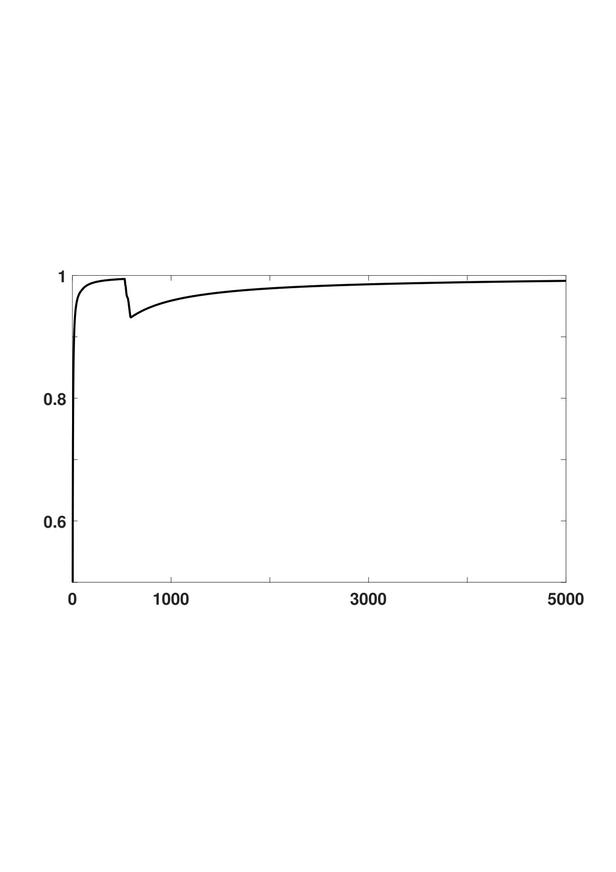 Figure 1
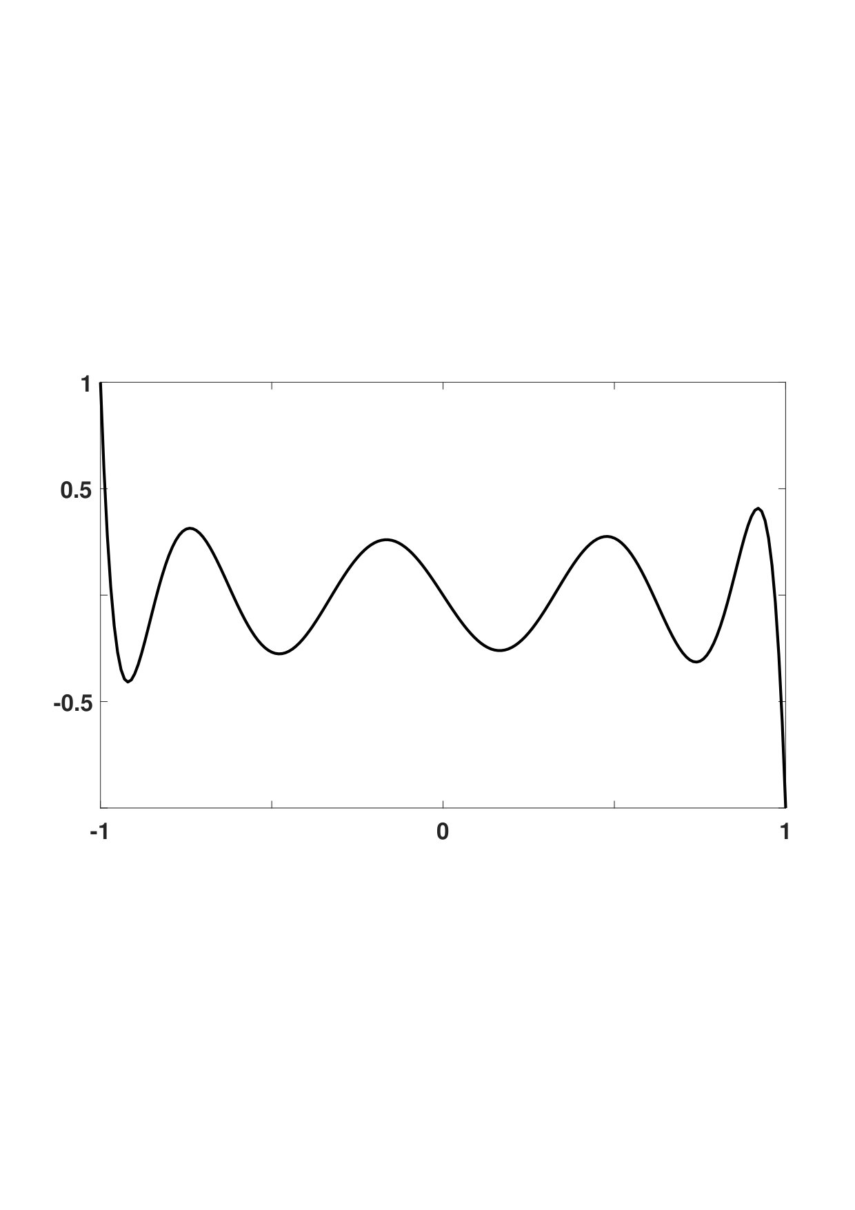 Figure 2
Peer Reviews
No public reviews on file for this paper yet. If you reviewed it on a platform where reviews are public (OpenReview, ICLR, NeurIPS, ICML), you can paste yours below so the community can read it here.
Videos
No videos yet. Explain this paper in a talk, walkthrough, or lecture? Add one.
Taxonomy
TopicsMarkov Chains and Monte Carlo Methods · Point processes and geometric inequalities · Geometric Analysis and Curvature Flows
11institutetext: Laboratoire IMS (CNRS 5218), Université de Bordeaux 11email: [email protected]
22institutetext: Department of Electrical and Electronic Engineering,
The University of Melbourne
22email: [email protected]
The Riemannian barycentre as a
proxy for global optimisation
Salem Said 11
Jonathan H. Manton 22
Abstract
Let be a simply-connected compact Riemannian symmetric space, and a twice-differentiable function on , with unique global minimum at . The idea of the present work is to replace the problem of searching for the global minimum of , by the problem of finding the Riemannian barycentre of the Gibbs distribution . In other words, instead of minimising the function itself, to minimise , where denotes Riemannian distance. The following original result is proved : if is invariant by geodesic symmetry about , then for each ( the convexity radius of ),
there exists such that implies is strongly convex on the geodesic ball , and is the unique global minimum of . Moreover, this can be computed explicitly. This result gives rise to a general algorithm for black-box optimisation, which is briefly described, and will be further explored in future work.
Keywords:
Riemannian barycentre black-box optimisation symmetric space.
It is common knowledge that the Riemannian barycentre , of a probability distribution defined on a Riemannian manifold , may fail to be unique. However, if is supported inside a geodesic ball with radius ( the convexity radius of ), then is unique and also belongs to . In fact, Afsari has shown this to be true, even when (see [1][2]).
Does this statement continue to hold, if is not supported inside , but merely concentrated on this ball? The answer to this question is positive, assuming that is a simply-connected compact Riemannian symmetric space, and , where the function has unique global minimum at . This is given by Proposition 2, in Section 2 below.
Proposition 2 motivates the main idea of the present work : the Riemannian barycentre of can be used as a proxy for the global minimum of . In general, only provides an approximation of , but the two are equal if is invariant by geodesic symmetry about , as stated in Proposition 3, in Section 4 below.
The following Section 1 introduces Proposition 1, which estimates the Riemannian distance between and , as a function of .
1 Concentration of the barycentre
Let be a probability distribution on a complete Riemannian manifold . A (Riemannian) barycentre of is any global minimiser of the function
[TABLE]
The following statement is due to Karcher, and was improved upon by Afsari [1][2] : if is supported inside a geodesic ball , where and ( the convexity radius of ), then is strongly convex on , and has a unique barycentre .
On the other hand, the present work considers a setting where is not supported inside , but merely concentrated on this ball. Precisely, assume is equal to the Gibbs distribution
[TABLE]
where is a normalising constant, is a function with unique global minimum at , and is the Riemannian volume of . Then, let denote the function in (1), and let denote any barycentre of .
In this new setting, it is not clear whether is differentiable or not. Therefore, statements about convexity of and uniqueness of are postponed to the following Section 2. For now, it is possible to state the following Proposition 1. In this proposition, denotes Riemannian distance, and denotes the Kantorovich (-Wasserstein) distance [3][4]. Moreover, is any open interval which contains the spectrum of the Hessian , considered as a linear mapping of the tangent space .
Proposition 1
*assume is an -dimensional compact Riemannian manifold with non-negative sectional curvature. Denote the Dirac distribution at . The following hold,
(i) for any ,*
[TABLE]
(ii) for (which can be computed explicitly)
[TABLE]
where in terms of the Beta function.
Proposition 1 is motivated by the idea of using as an approximation of . Intuitively, this requires choosing so small that is sufficiently close to . Just how small a may be required is indicated by the inequality in (4). This inequality is optimal and explicit, in the following sense.
It is optimal because the dependence on in its right-hand side cannot be improved. Indeed, by the multi-dimensional Laplace approximation (see [5], for example), the left-hand side is equivalent to (in the limit ). While this constant is not tractable, the constants appearing in Inequality (4) depend explicitly on the manifold and the function . In fact, this inequality does not follows from the multi-dimensional Laplace approximation, but rather from volume comparison theorems of Riemannian geometry [6].
In spite of these nice properties, Inequality (4) does not escape the curse of dimensionality. Indeed, for fixed , its right-hand side increases exponentially with the dimension (note that decreases like ). On the other hand, although also depends on , it is typically much less affected by dimensionality, and decreases slower that as increases.
2 Convexity and uniqueness
Assume now that is a simply-connected, compact Riemannian symmetric space. In this case, for any , the function turns out to be throughout . This results from the following lemma.
Lemma 1
let be a simply-connected compact Riemannian symmetric space. Let be a geodesic defined on a compact interval . Denote the union of all cut loci for . Then, the topological dimension of is strictly less than . In particular, is a set with volume equal to zero.
Remark : the assumption that is simply-connected cannot be removed, as the conclusion does not hold if is a real projective space.
The proof of Lemma 1 uses the structure of Riemannian symmetric spaces, as well as some results from topological dimension theory [7] (Chapter VII). The notion of topological dimension arises because it is possible is not a manifold. The lemma immediately implies, for all ,
[TABLE]
Then, since the domain of integration avoids the cut loci of all the , it becomes possible to differentiate under the integral. This is used in obtaining the following (the assumptions are the same as in Lemma 1).
Corollary 1
for , let and , where is the function . The following integrals converge for any
[TABLE]
and both depend continuously on . Moreover,
[TABLE]
so that is throughout .
With Corollary 1 at hand, it is possible to obtain Proposition 2, which is concerned with the convexity of and uniqueness of . In this proposition, the following notation is used
[TABLE]
where for positive . The reader may wish to note the fact that decreases to [math] as decreases to [math].
Proposition 2
*let be a simply-connected compact Riemannian symmetric space. Let be the maximum sectional curvature of , and its convexity radius. If (see (ii) of Proposition 1), then the following hold for any .
(i) for all in the geodesic ball ,*
[TABLE]
*where and is a constant given by the structure of the symmetric space .
(ii) there exists (which can be computed explicitly), such that implies is strongly convex on , and has a unique global minimum . In particular, this means is the unique barycentre of .*
Note that (ii) of Proposition 2 generalises the statement due to Karcher [1], which was recalled in Section 1.
3 Finding and
Propositions 1 and 2 claim that and can be computed explicitly. This means that, with some knowledge of the Riemannian manifold and the function , and can be found by solving scalar equations. The current section gives the definitions of and .
In the notation of Proposition 1, let be small enough, so that,
[TABLE]
whenever , and consider the quantity
[TABLE]
where is defined as in (6). Note that decreases to [math] as decreases to [math], for fixed and . Now, it is possible to define as
[TABLE]
[TABLE]
Here, for , and , where is the surface area of a unit sphere .
With regard to Proposition 2, define as follows,
[TABLE]
for some arbitrary . Here, in the notation of (4), (6) and (7),
[TABLE]
where .
4 Black-box optimisation
Consider the problem of searching for the unique global minimum of . In black-box optimisation, it is only possible to evaluate for given , and the cost of this evaluation precludes numerical approximation of derivatives. Then, the problem is to find using successive evaluations of (hopefully, as few of these evaluations as possible).
Here, a new algorithm for solving this problem is described. The idea of this algorithm is to find using successive evaluations of , in the hope that will provide a good approximation of . While the quality of this approximation is controlled by Inequalities (3) and (4) of Proposition 1, in some cases of interest, is exactly equal to , for correctly chosen , as in the following proposition 3.
To state this proposition, let denote geodesic symmetry about (see [7]). This is the transformation of , which leaves fixed, and reverses the direction of geodesics passing through .
Proposition 3
assume that is invariant by geodesic symmetry about , in the sense that . If (see (ii) of Proposition 2), then is the unique barycentre of .
Proposition 3 follows rather directly from Proposition 2. Precisely, by (ii) of Proposition 2, the condition implies is strongly convex on , and . Thus, is the unique stationary point of in . But, using the fact that is invariant by geodesic symmetry about , it is possible to prove that is a stationary point of , and this implies .
The two following examples verify the conditions of Proposition 3.
Example 1 : assume is a complex Grassmann manifold. In particular, is a simply-connected, compact Riemannian symmetric space. Identify with the set of Hermitian projectors such that , where denotes the trace. Then, define for , where is a Hermitian positive-definite matrix with distinct eigenvalues. Now, the unique global minimum of occurs at , the projector onto the principal
-subspace of . Also, the geodesic symmetry is given by , where denotes reflection through the image space of . It is elementary to verify that is invariant by this geodesic symmetry. Example 2 : let be a simply-connected, compact Riemannian symmetric space, and a function on with unique global minimum at . Assume moreover that is invariant by geodesic symmetry about . For each , there exists an isometry of , such that . Then, has unique global minimum at , and is invariant by geodesic symmetry about .
Example 1 describes the standard problem of finding the principal subspace of the covariance matrix . In Example 2, the function is a known template, which undergoes an unknown transformation , leading to the observed pattern . This is a typical situation in pattern recognition problems.
Of course, from a mathematical point of view, Example 2 is not really an example, since it describes the completely general setting where the conditions of Proposition 3 are verified. In this setting, consider the following algorithm.
Description of the algorithm :
– input : % to find such , see Section 3
% symmetric Markov kernel
% initial guess for
– iterate : for
(1) sample
(2) compute
(3) reject with probability % then,
(4) % see definition (10) below
– until : does not change sensibly
– output : % approximation of
The above algorithm recursively computes the Riemannian barycentre of the samples generated by a symmetric Metropolis-Hastings algorithm (see [8]). Here, The Metropolis-Hastings algorithm is implemented in lines (1)--(3). On the other hand, line (4) takes care of the Riemannian barycentre. Precisely, if is a length-minimising geodesic connecting to , let
[TABLE]
This geodesic need not be unique.
The point of using the Metropolis-Hastings algorithm is that the generated eventually sample from the Gibbs distribution . The convergence of the distribution of to takes place exponentially fast. Indeed, it may be inferred from [8] (see Theorem 8, Page 36)
[TABLE]
where is the total variation norm, and verifies
[TABLE]
so the rate of convergence is degraded when is small.
Accordingly, the intuitive justification of the above algorithm is the following. Since the eventually sample from the Gibbs distribution , and the desired global minimum of is equal to the barycentre of (by Proposition 3), then the barycentre of the is expected to converge to .
It should be emphasised that, in the present state of the literature, there is no rigorous result which confirms this convergence . It is therefore an open problem, to be confronted in future work.
For a basic computer experiment, consider and let
[TABLE]
where is the Legendre polynomial of degree [9]. The unique global minimiser of is , and the conditions of Proposition 3 are verified, since is invariant by reflection in the axis, which is geodesic symmetry about .
Figure 2 shows the dependence of on , displaying multiple local minima and maxima. Figure 2 shows the algorithm overcoming these local minima and maxima, and converging to the global minimum , within iterations. The experiment was conducted with , and the Markov kernel obtained from the von Mises-Fisher distribution (see [10]). The initial guess is not shown in Figure 2.
In comparison, a standard simulated annealing method offered less robust performance, which varied considerably with the choice of annealing schedule.
5 Proofs
This section is devoted to the proofs of the results stated in previous sections.
As of now, assume that . There is nos loss of generality in making this assumption.
5.1 Proof of Proposition 1
[TABLE]
Proof of (ii) : let where is the injectivity radius of at , and is an upper bound on the sectional curvature of . Assume, in addition, is small enough so
[TABLE]
[TABLE]
Proof of second estimate : the Kantorovich distance between and the Dirac distribution is equal to the expectation of the distance to , with respect to [4]. Precisely,
[TABLE]
6 Proof of Lemma 1
Denote the connected component at identity of the group of isometries of . It will be assumed that is simply-connected and semisimple [7]. Any geodesic is of the form [7][11],
[TABLE]
In order to describe the set , denote the isotropy group of in , and the Lie algebra of . Let be an orthogonal decomposition, with respect to the Killing form of , and let be a maximal Abelian subspace of . Define ( the centraliser of in ), and consider the mapping
[TABLE]
The set is the image under of a certain set , which is now described, following [7][12].
Let be the set of positive restricted roots associated to the pair , (each is a linear form ). Then, let be the set of such that for all , and the boundary of . Then
[TABLE]
Recapitulating (17b) and (17d),
[TABLE]
Lemma 1 states that the topological dimension of is strictly less than . This is proved using results from topological dimension theory [7][13].
Note that both and are compact. Indeed, is compact since it is the continuous image of the compact group under the projection . Also, is compact in , and where for . Since is the union of two (closed) hyperplanes in , is compact. Now, each is compact, and therefore closed. It follows from (17e) that (see [13], Page 30),
[TABLE]
But, for each ,
[TABLE]
where ( the centraliser of in ). The above inclusion implies (by [13], Page 26),
[TABLE]
To conclude, note that the set is a differentiable manifold. It follows that (see [7], Page 345),
[TABLE]
The right-hand side of this inequality is
[TABLE]
since the dimension of a hyperplane in is . In addition, according to [7] (Page 296), . Thus,
[TABLE]
since [7]. Replacing this into (17h), it follows from (17f) and (17g) that , as required.
7 Proof of Corollary 1
The corollary can be split into the two following claims, which will be proved separately.
First claim : both integrals and converge for any value of .
Second claim : is throughout , with derivatives given by (5).
The fact that and depend continuously on is contained in the second claim, since (5) states that and are the gradient and Hessian of at .
In the following proofs, the notation will be used, in order to avoid cumbersome expressions.
Proof of first claim : The convergence of the integral is straightforward, since the integrand is a smooth and bounded function, from to . This is because, by definition, is given by
[TABLE]
[TABLE]
The convergence of the integral is more difficult. While the integrand is smooth on , it is not bounded. It will be seen that is an absolutely convergent improper integral.
Recall the mapping defined in (17c). Let be the set of points which belong to the interior of , and which verify for each . Let be the interior of . Then, maps onto , and is a diffeomorphism of onto its image in [7][12] (see Chapter VII in [7]). Using Sard’s theorem [14], it follows from the definition of that
[TABLE]
where denotes the density of with respect to the Riemannian volume of , and is the Jacobian determinant of , given by [7]
[TABLE]
with the multiplicity of the restricted root , and where is the invariant Riemannian volume induced on from .
Now, can be expressed as follows ( is the cotangent function)
[TABLE]
where and the denote orthogonal projectors, onto the respective eigenspaces of .
According to this expression, diverges to whenever . However, the product
[TABLE]
which appears under the integral in (19a), is clearly continuous and bounded on the domain of integration. Thus, the absolute convergence of the integral follows immediately from (19a).
It now remains to provide a proof of (19c). This is here only briefly indicated. Expression (19c) is a slight improvement of the one in [15] (see Theorem IV.1, Page 636), where it is enough to note that if is the curvature tensor of , then the operator has the eigenvalues [math] and for each , whenever with [7][12]. It is well-known, by properties of the Jacobi equation [6], that has the same eigenspace decomposition as , in this case. Proof of second claim : the proof of this claim relies in a crucial way on Lemma 1. To compute the gradient and Hessian of the function at , consider any geodesic , defined on a compact interval , such that . For each , by definition of the function ,
[TABLE]
Then, consider the integral , and recall Formulae (19a) and (19c). Each can be written under the form where . Accordingly, it follows from (19c) that
[TABLE]
where is the Frobenius norm with respect to the Riemannian metric of , and is the highest restricted root [7] ( for , ).
The required uniform integrability is equivalent to the statement that
[TABLE]
where the rate of convergence to this limit does not depend on . But, according to (20d), if , there exists such that
[TABLE]
and as . In this case, the integral in (20e) is less than
[TABLE]
Now, using the same integral formula as in (19a), this last integral is equal to
[TABLE]
In view of (19b), since , the function in square brackets is bounded on the closure of . In fact [7], its supremum is where is the scalar product induced on (the dual space of by the Killing form of . Finally, by (20f), the integral in (20e) is less than
[TABLE]
Since, for , this last integral converges to [math] as , at a rate which does not depend on . This proves the required uniform integrability, so the proof is now complete.
8 Proof of Proposition 2
[TABLE]
Remark : in the statement of Proposition 2, the notation is used for the maximum sectional curvature of . In the previous proof of Corollary 1, the same notation was used for the squared norm of the highest restricted root. This is not an abuse of notation, since the two quantities are in fact equal [7] (see Page 334).
Proof of (i) : let . By (5) of Corollary 1, is equal to . To obtain (7), decompose into two integrals
[TABLE]
This is possible since , where . The first integral in (21a) will be denoted , and the second integral .
With regard to , note the inclusions , which follow from the triangle inequality. In addition, note that (in the Loewner order [16]), for . Therefore,
[TABLE]
However, from (19c) and the definition of ,
[TABLE]
for . Using the Cauchy-Scwharz inequality, . Moreover, (17c) implies , since is an isometry. Accordingly, if , it follows from (21c)
[TABLE]
where the last inequality is because . Replacing in (21b) gives
[TABLE]
Finally, (15c) and (15d) imply that , where was defined in (6) – Precisely, this follows after replacing by in (15c). Thus,
[TABLE]
The proof of (7) will be completed by showing
[TABLE]
Proof of (ii) : fix , and let be given by (9). If , then , so the definition of implies
[TABLE]
By (i) of Proposition 1, to prove that , it is enough to prove
[TABLE]
However, if , then . Therefore, by (ii) of Proposition 1, satisfies inequality (4). Furthermore, because , it follows from the definition of that
[TABLE]
or, by replacing the expression of , and simplifying
[TABLE]
Thus, (23c) follows from (4) and (23d). This proves that belongs to , and therefore is the unique global minimum of . But this is equivalent to saying that is the unique barycentre of .
9 Proof of Proposition 3
fix , and let be given by (9). By (ii) of Proposition 2, if , then is strictly convex on , with unique global minimum . By definition, this unique global minimum is the unique barycentre of .
Accordingly, to prove that , it is enough to prove that is a stationary point of . Indeed, as is strictly convex on , it can have only one stationary point in . This stationary point is then identical to .
The fact that is a stationary point of will follow because is invariant by geodesic symmetry about . This invariance will be seen to imply
[TABLE]
To obtain (24a), it is possible to write, from the definition of ,
[TABLE]
where . From (18), since is an isometry, and reverses geodesics passing through ,
[TABLE]
Replacing this into (24b), and using as a new variable of integration, it follows that
[TABLE]
because and maps onto itself. Now, note that . This is clear, since from (2),
[TABLE]
However, by assumption, . Moreover, since is an isometry, it preserves Riemannian volume, so . Thus, (24c) reads
[TABLE]
By definition, the right-hand side is , so (24a) is obtained.
The reference list from the paper itself. Each links out to its DOI / PubMed record.
- 1[1] Karcher, H.: Riemannian centre of mass and mollifier smoothing. Comm. Pure. Appl. Math. 30 (5), 509–541 (1977).
- 2[2] Afsari, B.: Riemannian L p superscript 𝐿 𝑝 L^{p} center of Mass : existence, uniqueness, and convexity. Proc. Am. Math. Soc. 139 (2), 655–673 (2010).
- 3[3] Kantorovich, L.V., Akilov, G.P. : Functional Analysis (Second Edition). Pergamon Press, Oxford (1982).
- 4[4] Villani, C.: Optimal transport, old and new. 2nd edn. Springer-Verlag, Berlin-Heidelberg (2009).
- 5[5] Wong, R.: Asymptotic approximations of Integrals. Society for Industrial and Applied Mathematics (2001).
- 6[6] Chavel, I.: Riemannian Geometry, a modern introduction. Cambridge University Press, Cambridge (2006).
- 7[7] Helgason, S.: Differential geometry, Lie groups, and symmetric spaces. American Mathematical Society (1978).
- 8[8] Roberts, G. O., Rosenthal, J. S.: General state space Markov chains and MCMC algorithms. Probab. Surveys. 1 , 20–71 (2004).