Stratified communities in complex business networks
Roy Cerqueti, Gian Paolo Clemente, and Rosanna Grassi

TL;DR
This paper introduces a new way to analyze community structures in networks by considering stratification levels, extending clustering coefficients, and applying the method to business and air traffic networks for validation.
Contribution
It proposes a novel local $l$-adjacency clustering coefficient that accounts for community stratification, enhancing community detection insights.
Findings
Validated on air traffic networks, demonstrating practical usefulness.
Extended clustering coefficient provides deeper community structure insights.
Empirical analysis supports the theoretical framework.
Abstract
This paper presents a new definition of the community structure of a network, which takes also into account how communities are stratified. In particular, we extend the standard concept of clustering coefficient and provide the local -adjacency clustering coefficient of a node . We define it as an opportunely weighted mean of the clustering coefficients of nodes which are at distance from . The stratus of the community associated to node is identified by the distance from , so that the standard clustering coefficient is a peculiar local -adjacency clustering coefficient at stratus . As the distance varies, the local -adjacency clustering coefficient is then used to infer insights on the community structure of the entire network. Empirical experiments on special business networks are carried out. In particular, the analysis of air traffic networks…
Click any figure to enlarge with its caption.
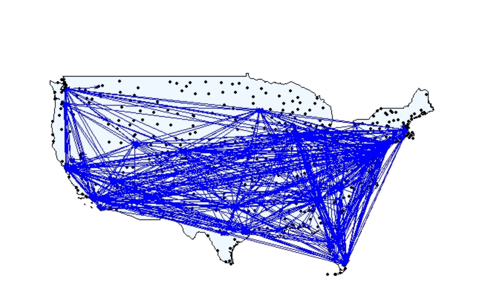 Figure 1
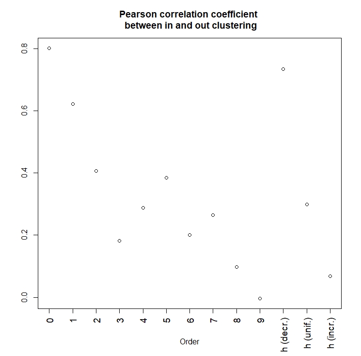 Figure 2
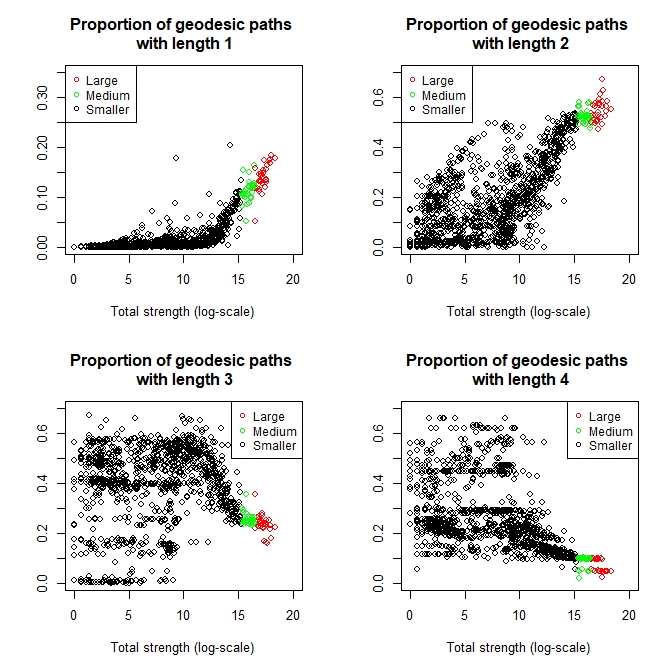 Figure 3
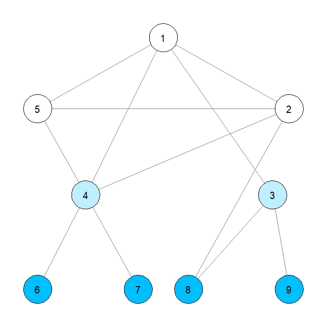 Figure 4
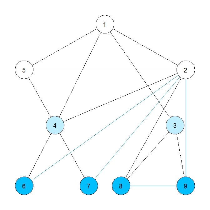 Figure 5
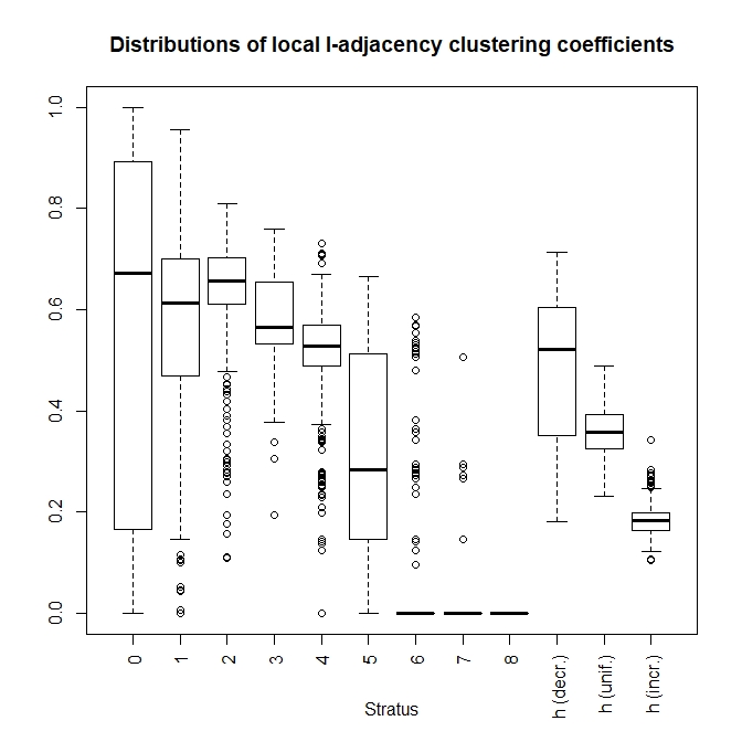 Figure 6
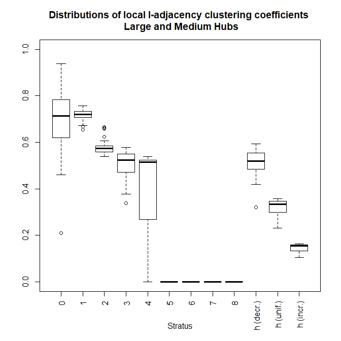 Figure 7
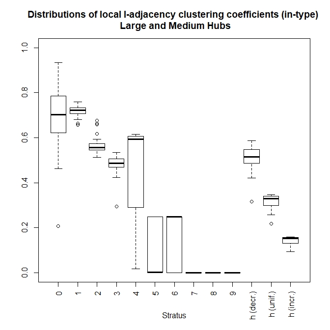 Figure 8
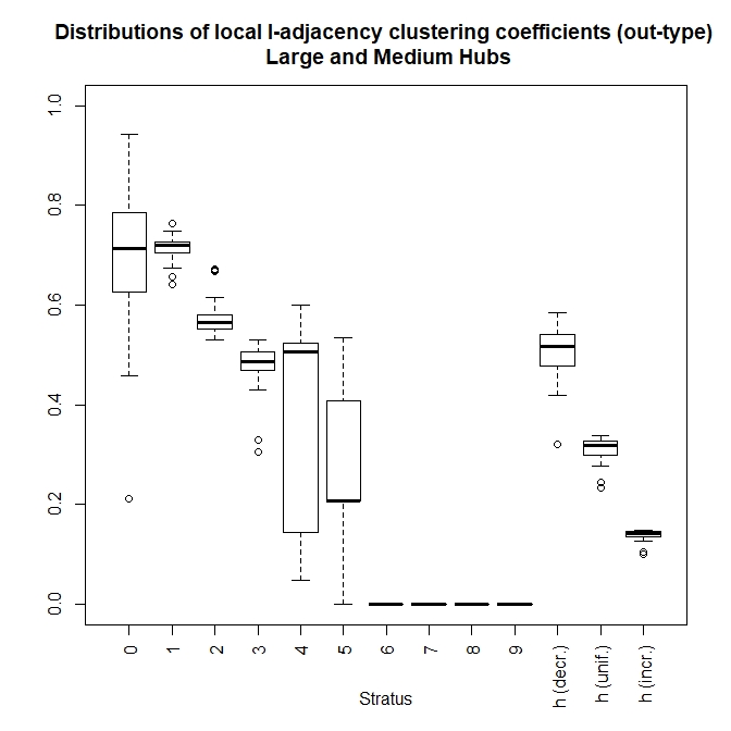 Figure 9
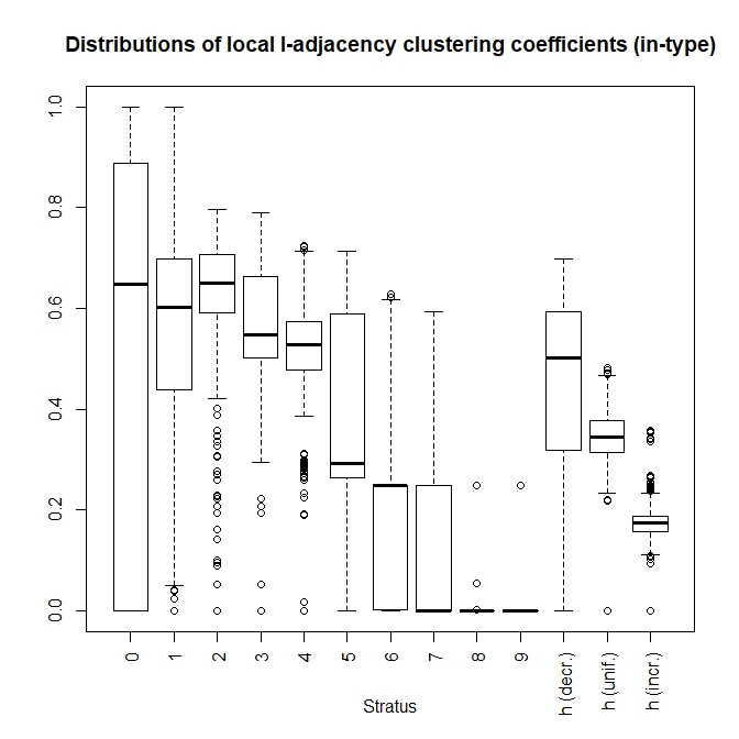 Figure 10
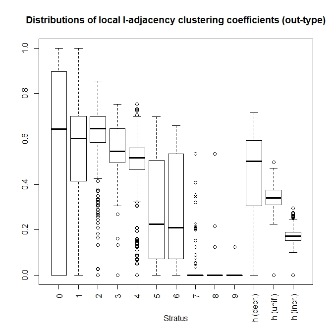 Figure 11
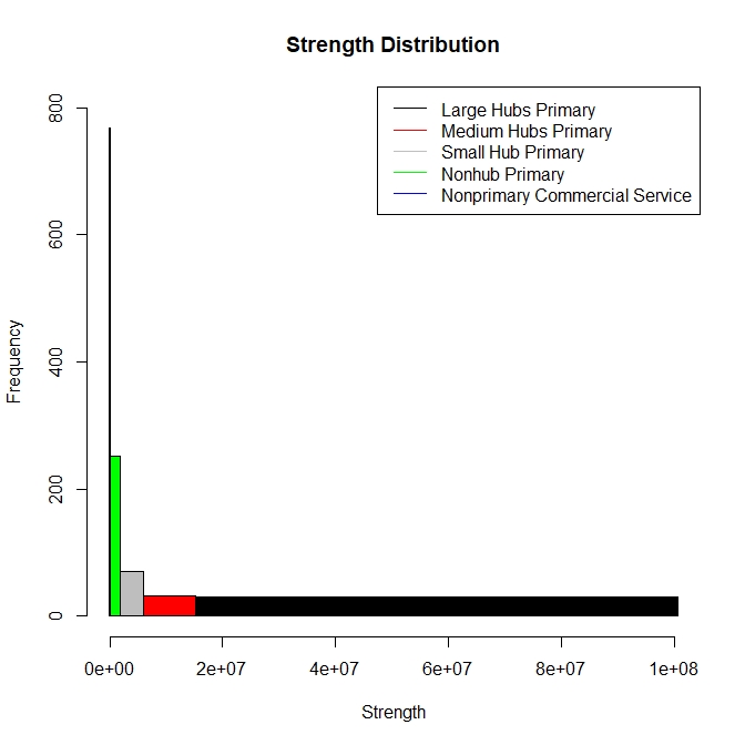 Figure 12
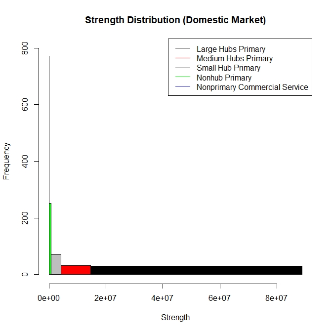 Figure 13
| Node | ||||||||
|---|---|---|---|---|---|---|---|---|
| Decreasing Weights | Uniform Weights | Increasing Weights | ||||||
| 1 | 0.50 | 0.45 | 0 | 0 | 0 | 0.32 | 0.19 | 0.09 |
| 2 | 0.50 | 0.45 | 0 | 0 | 0 | 0.32 | 0.19 | 0.09 |
| 3 | 0 | 0.17 | 0.60 | 0 | 0 | 0.12 | 0.15 | 0.11 |
| 4 | 0.30 | 0.40 | 0 | 0 | 0 | 0.22 | 0.14 | 0.07 |
| 5 | 1 | 0.43 | 0 | 0 | 0 | 0.53 | 0.29 | 0.14 |
| 6 | 0 | 0.30 | 0.50 | 0 | 0 | 0.14 | 0.16 | 0.11 |
| 7 | 0 | 0.30 | 0.50 | 0 | 0 | 0.14 | 0.16 | 0.11 |
| 8 | 0 | 0.25 | 0.45 | 0 | 0 | 0.12 | 0.14 | 0.09 |
| 9 | 0 | 0 | 0.25 | 0.60 | 0 | 0.10 | 0.17 | 0.17 |
| Node | |||||||
|---|---|---|---|---|---|---|---|
| Decreasing Weights | Uniform Weights | Increasing Weights | |||||
| 1 | 0.50 | 0.53 | 0.83 | 0 | 0.50 | 0.47 | 0.34 |
| 2 | 0.29 | 0.76 | 0.33 | 0 | 0.37 | 0.35 | 0.24 |
| 3 | 0.33 | 0.61 | 0.60 | 1 | 0.52 | 0.63 | 0.76 |
| 4 | 0.50 | 0.76 | 0.56 | 0 | 0.51 | 0.45 | 0.31 |
| 5 | 1 | 0.43 | 0.73 | 0 | 0.70 | 0.54 | 0.36 |
| 6 | 1 | 0.39 | 0.77 | 0.33 | 0.74 | 0.62 | 0.53 |
| 7 | 1 | 0.39 | 0.77 | 0.33 | 0.74 | 0.62 | 0.53 |
| 8 | 0.67 | 0.43 | 0.80 | 0 | 0.55 | 0.47 | 0.34 |
| 9 | 0.67 | 0.43 | 0.80 | 0 | 0.55 | 0.47 | 0.34 |
| Rank | City | Airport Name |
|---|---|---|
| 1 | Atlanta | Hartsfield - Jackson Atlanta International |
| 2 | Los Angeles | Los Angeles International |
| 3 | Chicago | Chicago O’Hare International |
| 4 | Fort Worth | Dallas-Fort Worth International |
| 5 | Denver | Denver International |
| 6 | New York | John F Kennedy International |
| 7 | San Francisco | San Francisco International |
| 8 | Las Vegas | McCarran International |
| 9 | Seattle | Seattle-Tacoma International |
| 10 | Charlotte | Charlotte/Douglas International |
| 11 | Newark | Newark Liberty International |
| 12 | Orlando | Orlando International |
| 13 | Phoenix | Phoenix Sky Harbor International |
| 14 | Miami | Miami International |
| 15 | Houston | George Bush Intercontinental/Houston |
| 16 | Boston | General Edward Lawrence Logan International |
| 17 | Minneapolis | Minneapolis-St. Paul International/Wold-Chamberlain |
| 18 | Detroit | Detroit Metropolitan Wayne County |
| 19 | Fort Lauderdale | Fort Lauderdale/Hollywood International |
| 20 | New York | Laguardia |
| 21 | Philadelphia | Philadelphia International |
| 22 | Glen Burnie | Baltimore/Washington International Thurgood Marshall |
| 23 | Salt Lake City | Salt Lake City International |
| 24 | Arlington | Ronald Reagan Washington National |
| 25 | San Diego | San Diego International |
| 26 | Dulles | Washington Dulles International |
| 27 | Chicago | Chicago Midway International |
| 28 | Honolulu | Daniel K. Inouye International |
| 29 | Tampa | Tampa International |
| 30 | Portland | Portland International |
| Rank | City | Airport Name |
|---|---|---|
| 31 | Dallas | Dallas Love Field |
| 32 | St. Louis | St Louis Lambert International |
| 33 | Nashville | Nashville International |
| 34 | Austin | Austin-Bergstrom International |
| 35 | Houston | William P. Hobby |
| 36 | Oakland | Metropolitan Oakland International |
| 37 | San Jose | Norman Y. Mineta San Jose International |
| 38 | Metairie | Louis Armstrong New Orleans International |
| 39 | Raleigh | Raleigh-Durham International |
| 40 | Kansas City | Kansas City International |
| 41 | Sacramento | Sacramento International |
| 42 | Santa Ana | John Wayne Airport-Orange County |
| 43 | Cleveland | Cleveland-Hopkins International |
| 44 | San Antonio | San Antonio International |
| 45 | Fort Myers | Southwest Florida International |
| 46 | Indianapolis | Indianapolis International |
| 47 | Pittsburgh | Pittsburgh International |
| 48 | San Juan | Luis Munoz Marin International |
| 49 | Greater Cincinnati | Cincinnati/Northern Kentucky International |
| 50 | Columbus | John Glenn Columbus International |
| 51 | Kahului | Kahului |
| 52 | Milwaukee | General Mitchell International |
| 53 | Windsor Locks | Bradley International |
| 54 | West Palm Beach | Palm Beach International |
| 55 | Jacksonville | Jacksonville International |
| 56 | Anchorage | Ted Stevens Anchorage International |
| 57 | Albuquerque | Albuquerque International Sunport |
| 58 | Burbank | Bob Hope |
| 59 | Buffalo | Buffalo Niagara International |
| 60 | Ontario | Ontario International |
| 61 | Omaha | Eppley Airfield |
Peer Reviews
No public reviews on file for this paper yet. If you reviewed it on a platform where reviews are public (OpenReview, ICLR, NeurIPS, ICML), you can paste yours below so the community can read it here.
Videos
No videos yet. Explain this paper in a talk, walkthrough, or lecture? Add one.
Stratified communities in complex business networks
Roy Cerqueti*♭, Gian Paolo Clemente♮, Rosanna Grassi♯*
♭ University of Macerata, Department of Economics and Law.
Via Crescimbeni 20, 62100, Macerata, Italy.
Tel.: +39 0733 2583246; fax: +39 0733 2583205. Email: [email protected]
♮ Catholic University of Milan, Department of Mathematics, Finance and Econometrics
Email: [email protected]
♯ University of Milano-Bicocca, Department of Statistics and Quantitative Methods
Email: [email protected] Corresponding author.
Abstract
This paper presents a new definition of the community structure of a network, which takes also into account how communities are stratified. In particular, we extend the standard concept of clustering coefficient and provide the local -adjacency clustering coefficient of a node . We define it as an opportunely weighted mean of the clustering coefficients of nodes which are at distance from . The stratus of the community associated to node is identified by the distance from , so that the standard clustering coefficient is a peculiar local -adjacency clustering coefficient at stratus . As the distance varies, the local -adjacency clustering coefficient is then used to infer insights on the community structure of the entire network. Empirical experiments on special business networks are carried out. In particular, the analysis of air traffic networks validate the theoretical proposal and provide supporting arguments on its usefulness.
Keywords: Community structure, complex business networks, geodesic distance in networks, communities stratification.
1 Introduction
Business researchers and economists are paying a growing attention to the relevant theme of communities detection and to the related complex networks models, as recent literature suggests. In the area of financial economics, [1] deals with the clusters of networks of economies by using data on the Gross Domestic Product of a group of countries. Under an international economics perspective, [2, 18] discuss the assessment of the communities in the context of the world trade network. The theme of the brand communities in the framework of entrepreneurship and social science is also largely debated (see e.g. [7, 15, 24]). It is worth mentioning the role of communities in corporate organizations and firms cooperation (see e.g. [20, 23]). In general, a managerial architecture is grounded on the relationships among agents, and network structures are particularly effective in offering a representation of the complexity of the relationship among the involved actors. Firms and managers are usually interconnected through an intricate weave. Hence, discovering how they are clustered at every level of the structure can give useful insights in entrepreneurial strategic choices ([12, 23, 24]).
The community structure around a node is generally represented and measured through its clustering coefficient. Such a coefficient can be defined in an operative way, being computed as the relative number of actual triangles to which the vertex belongs over the hypothetical ones. It has been developed in all the cases of weighted, unweighted, directed and undirected networks. In this respect, we mention the classical contributions of [3, 10, 16, 22] and the non recent but highly informative monograph [21]. Recently, [5] contains a relevant extension of the clustering coefficient proposed by [10]; [19] discusses the clustering coefficient in presence of already established communities for directed networks; [4] presents a concept of clustering coefficient which also includes the presence of missing indirect links in the construction of the triangles. The association between communities and clustering coefficients is quite natural. Triangles are the easiest geometric visualizations of the communities, providing a picture of non-exclusive interactions among different agents. Clustering coefficient could be used then as an indicator of the node position with respect to communities. However, even if it describes the linkages around a vertex, this coefficient is a local measure hence it does not capture the topology of the whole network. Moreover, the global clustering coefficient of the network – which is simply obtained by taking the average of the local versions over all the nodes of the network – often is not very informative. Indeed, a network can be highly clustered at a local level but not at a global level, and this suggests that the average of local clustering could not well represent the global characteristics of the network. This drawback is peculiarly relevant, since it is often crucial to assess the position of a node with respect to communities in which the node itself is not directly involved (see [8]).
This paper extends the concept of community structure of a node by considering the role and the relevance of the communities which are placed at a geodesic distance from the considered node . In details, we define the local -adjacency clustering coefficient of a node as an opportunely weighted mean of the clustering coefficients of the nodes at geodesic distance from . In this way, we present a model of stratified communities, where the stratification is ruled by the varying geodesic distances from the reference node. In particular, the stratified community at stratus is defined through the clustering coefficients of the nodes at geodesic distance from . In this respect, the geodesic distance from the node represents the stratus of the community.
Assessing the stratified community structure of a network represents a crucial point for understanding the contextualization of the nodes within the overall system. For instance, assume that a node has a low clustering coefficient but the nodes at a distance from it exhibit a strong community level. In this case, the node is not embedded in a powerful community but it is surrounded by a high level of mutual interconnections for the nodes quite far from it. This situation can be interpreted under the perspective of shocks propagation. Indeed, if a node, located at a geodesic distance from greater than , receives a shock, such a shock could hardly reach , since is surrounded by highly clustered nodes at a large distance from it and by an empty space – in terms of connections – around it. In other words, nodes at distance might be viewed as a sort of barrier for , absorbing the external solicitations at larger distances. This stops the propagation to , because of the absence of a community structure close to the node.
To test the proposed measure we perform an empirical application to the paradigmatic business network related to the U.S. domestic air traffic. Findings confirm the effectiveness of these measures in seizing the peculiar characteristics of different hubs in the airport network. We observe that larger hubs are not only highly clustered but also connected to strong communities. When higher strati are analysed, the effects of indirect connections with remote airports are emphasized. Referring to large and medium hubs, the proposed approach allows to emphasize the strategic role of such nodes in the airport network system. Finally, although the considered empirical network is only weakly asymmetric and it is typically analysed as an undirected network in the literature (see, for instance, [3, 6, 5, 13, 14, 17]), we show that a separate evaluation of directed paths at high levels can be useful to identify specific patterns in terms of in- and out-communities.
The rest of the paper is organized as follows. In Section 2, we present the mathematical preliminaries and the basic notation used in the article. In Section 3, the concepts of local -adjacency clustering coefficient – being the stratus of the related community – is defined for both undirected and directed case. In Section 4 the new conceptualization of clustering coefficients is applied to the U.S. airport network, in order to discuss its stratified community structure. Conclusions are in Section 5.
2 Preliminary definitions and notations
We briefly present the mathematical definitions used in the paper. A graph is identified by a set of vertices and a set of unordered pairs of vertices (called edges). Vertices and are said to be adjacent if . Graphs considered here will be always without loops. The degree of the vertex is the number of its adjacent nodes. A path between two vertices and is a sequence of distinct vertices and edges between and . In this case, and are connected. is connected if every pair of vertices is connected. The distance is the length of any shortest path (or geodesic) between and . If and are not connected, then . The diameter of a connected graph is the length of any longest geodesic.
Given a connected graph , we define the set:
[TABLE]
of nodes which are at distance with respect to the node , where . The cardinality is denoted as . Notice that is the set of nodes adjacent to , so that .
A graph is weighted when a positive real number is associated with the edge . if nodes and are not adjacent. In particular, when if , then the graph is unweighted. Thus, the unweighted case can be viewed as a particular weighted one. For this reason, we use in this paper only the general concept of weighted graphs and we denote a weighted graph with its weights simply as weighted network.
The strength of the vertex is defined as .
In general, both adjacency relationships between vertices of and weights on the edges are described by a nonnegative, real -square matrix (the weighted adjacency matrix), with entries .
A weight can be also associated to every geodesic of a connected graph in the following way: let be the set of the geodesics connecting the vertices and ; the generic element of is .
We observe that more than one geodesic connecting and could exist, so that, in general, . Recalling that all the geodesics in have the same length, a unique integer exists such that the length of all the paths in is . The role of is crucial for the following arguments. Therefore, will be explicitly added in the notation when needed so that, for instance, will be , will become and so on.
The weight of is the sum of the weights of its edges and we denote it with . This allows us to define the -th order strength of the node in this setting as
[TABLE]
where Notice that when , then ; hence and is the strength of the vertex .
A directed graph is obtained from by adding to its edges a direction and is the underlying graph of . In this case, the links between couples of nodes are called directed edges or arcs. In a weighted directed graph, a weight is associated with the directed edge and, in general, the matrix is not symmetric. In fact, since bidirectional edges between a pair of nodes can exist, both and can be positive with .
A directed path from to is a sequence of distinct vertices and arcs from to such that every arc has the same direction; in this case, we say that is reachable from and we call this out-path of the node . The distance from to is the length of such shortest out-path (or out-geodesic) if any, otherwise .
Since directed paths from to can also exist, we define the in-path of the node as the directed path from to and we denote with the length of any shortest such in-path (or in-geodesic). If is not reachable from , then .
If and are mutually reachable, both in and out-geodesics of exist, although the distances and can be different. is strongly connected if every two vertices are mutually reachable.
is weakly connected if the underlying graph is connected. That it means that a geodesic between and exists in the underlying graph . In this case, distance is finite for all .
In addition, we define the following sets:
, for each ; 2. 2.
, for each .
Moreover, according to what we did above, we can define and as the sets of the out-geodesics and in-geodesics connecting the vertices and , respectively; the generic elements of and are and , respectively.
Hence, the definition of weighted in- and out-geodesics can be easily given by setting:
; 2. 2.
.
This allows us to define the -th order in and out-strength of the node as
[TABLE]
[TABLE]
3 Stratified communities
The aim of this section is to define a new indicator of community structure around a node based on the mutual interconnections between nodes at different distances from . This new indicator uses an extended idea of clustering coefficient, moving along shortest paths. Hence, we are providing a conceptualization of the stratified communities around the nodes of a network.
We introduce the indicator discussing separately the undirected and directed case.
3.1 Local -adjacency clustering coefficient: undirected case
Let for be the matrix such that:
[TABLE]
For the sake of completeness, the definition of the matrix can be extended to the case , by setting , being the identity matrix.
We define the vector of the local -adjacency clustering coefficients of the nodes of the network , as:
[TABLE]
where is the vector whose element is the weighted clustering coefficient of node , defined in Barrat et al. ([3]).
Notice that, when , formula (2) gives , and then we recover the weighted local clustering coefficient defined in [3].
When , the local -adjacency clustering coefficient is the vector of elements:
[TABLE]
where each element represents the weighted average of the clustering coefficients of the nodes which are adjacent to . This is true also for , as in general, formula (2) states that is the weighted average, with weights , of clustering coefficients of nodes which are at distance with respect to the node . Furthermore, it is noteworthy that, in case of an unweighted graph, the coefficient reduces to a classic arithmetic mean.
The elements of the vector defined in (2) give insights about the community structure at a specific distance from nodes of the graph. Indeed, the element associated to the proposed definition of the clustering coefficient explains how the nodes at distance from form a community in the graph.
Large values of such clustering coefficients of at high levels suggest that is connected with well-established communities which are far from the node itself. In other words, the analysis of with leads to a complete view of the graphs in terms of spatial communities, and this might give insights on how shocks propagate. The quantity describes the community structure at stratus around the node and the set of vectors defines the stratified community structure of the network as the value of varies.
In order to measure the overall community structure around a node , we then introduce the vector such that
[TABLE]
where , for each , and .
The vector allows tracking the whole community structure around a single node , and takes into account all the strati. Notice that the selection of a peculiar distribution of the weights provides the meaning of the concept of stratified community for all the nodes of the graph. In particular, high polarization of such a distribution at low (high) level leads to core-based (periphery-based) identification of the community structure. The special case focuses attention only to communities at stratus .
3.2 Local -adjacency clustering
coefficients: directed case
We consider a directed, weighted and weakly connected graph .
As already pointed out in Section 2, in addition to weighted paths, also weighted in- and out-paths can exist and we can focus only on a specific pattern (out-path or in-path for the node ), or we can consider all edges’ directions. Each choice is reasonable and depends on the kind of problem we deal with.
For , we define the matrix with the following entries:
[TABLE]
where:
, and if only out-paths of node are considered. In this case, will be denoted by ;
, and if only in-paths of node are considered. In this case, will be denoted by ;
, and if all the directions of the edges are taken into account. In this case, will be denoted by .
Also in this case, we set .
The definition of local -adjacency clustering coefficients, introduced in formula (2) has to be extended to the three cases , and .
Indeed, in the specific context of directed graphs, edges pointing in different directions have a completely different interpretation in terms of the resulting flow pattern. To this aim, alternative in-type or out-type local -adjacency clustering coefficients can be also obtained as:
[TABLE]
[TABLE]
where and are matrices defined in formula (5) whose elements are computed considering only in-paths (case ) or out-paths (case ), respectively. and are the vectors whose elements and are the in and out local local clustering coefficients defined in [5]. These two coefficients convey information about clustering of two different patterns (in or out) within tightly connected directed neighbourhoods.
According to the case , we define the local -adjacency clustering coefficients as:
[TABLE]
where is the vector whose elements are the weighted and directed clustering coefficients provided in [5].
The difference between the vectors of local -adjacency clustering coefficients in (2) and (8) lies in the considered definition of triangles. The same triple of nodes might be associated to one triangle (no directions of the arcs to be taken into account) in the former case and two of them (two possible directions for the arcs) in the latter one. In the special case of absence of bilateral arcs, the following result holds true:
Proposition 1**.**
Let D be a directed graph. If the graph has not bilateral arcs, then , where is the vector of the local -adjacency clustering coefficients of the undirected underlying graph .
Proof.
We define and the weighted adjacency matrices of the graphs and . The local clustering coefficient for weighted and directed network is defined as (see [5]):
[TABLE]
where and are respectively the total strength and the degree of the node , whereas is the strength related to bilateral arcs between and its adjacent nodes.
Since the graph has not bilateral arcs, . Additionally, if nodes and are adjacent, a (unique) weighted arc between and exists so that if then or vice versa. As a consequence, and .
Furthermore,
[TABLE]
A similar chain of equalities entails that .
Hence, (9) yields, :
[TABLE]
and, by formula (8):
[TABLE]
∎
Analogously to formula (4), we can define , , and , where:
[TABLE]
3.3 How the local -adjacency clustering
coefficients work: an illustrative example
The classical clustering coefficient does not give insights on both the topological structure and the stratified community structure of the whole network, being a measure of the local community structure concentrated around the nodes of the network. For the same reason also the global clustering coefficient of the network, which is given by the average of the local version around the nodes, is often not very informative. Furthermore, a network can be highly clustered at a local level but not on a global level, so that the average of the local clustering could not well represent the global characteristics of the network (see [8]).
To illustrate how the local -adjacency clustering coefficients effectively map the communities structure in the network, we show how they work by comparing two small graphs. For the sake of simplicity, we limit our investigation to undirected and unweighted graphs, as interesting remarks can be done also in this very simplified, but meaningful, case.
Let us consider the two graphs and , sharing the same number of nodes (namely, 9) and same diameter (namely, 4), but different topology, having more arcs than (hence, showing a stronger community structure, see Figure 1). In both graphs, node 1 shares the same neighbours and, being part of the same triangles, it has the same clustering coefficient . This coefficient is then not effective in capturing the actual position of the node with respect to the communities in the network. Indeed, the classical clustering coefficient gives insights about how the node 1 is embedded in a cohesive group only respect to its neighbours.
To have a more reliable information about how the node is located in respect to the whole structure, in particular to existing communities, we need to analyse its position looking deeper than its neighbours and the -adjacency clustering coefficients (with ) in this sense are meaningful.
Comparing the values of the clustering coefficients in Tables 1 and 2, the coefficient of node 1 decreases with respect to in the case of (from 0.5 to 0) moving through paths of length greater than 1, whereas in case it increases till (from 0.5 to 0.83) and becomes null for .
Therefore, the different strati of the community structure around the node 1 well reflect the position of such a node with respect to the way the other nodes are connected in the structure.
Through elements we are able to simultaneously consider all the communities at the different strati. We control the impact of each coefficient through their weights . We consider here three possible scenarios for the weights ’s:
- •
Decreasing weights: where is the harmonic number of order , for each ;
- •
Uniform weights: , for each ;
- •
Increasing weights: , for each .
Intuitive interpretations of the weights arise. Decreasing weights, for instance, reduce the impact on the node of high distances when assessing the community. Notice that, the elements in do not provide similar information of the classical average clustering coefficient. Instead, we are measuring the position of the node inside the network looking at each stratus. These indicators then provide an overall look and, at the same time, they track the node distances from the communities in the network.
4 Empirical experiments
In order to see how the proposed indicator is effective in describing the stratified communities of a node, we test it on the peculiar business network of the U.S. airport, where nodes are the airports and arcs are weighted on the basis of the flights scheduled among them in a given year. The considered reference year in the proposed experiments is 2017. The network is constructed by using the Air Carrier Statistics database (available on the U.S. Department of Transportation111Data are collected by the Office of Airline Information, Bureau of Transportation Statistics, Research and Innovative Technology Administration.), also known as the T-100 data bank, that contains domestic and international airline market and segment data. Both certificated U.S. air carriers and foreign carriers (having at least one point of service in the United States or one of its territories) report monthly traffic information. The weight of an arc corresponds to the number of emplaned passengers222The term “emplaned passengers”, widely used in the aviation industry, refers to passengers boarding a plane at a particular airport. Since the majority of airport revenues are generated, directly or indirectly, by emplaned passengers, this number is the most important air traffic metric. Data consider the total number of revenue passengers boarding an aircraft (including originating, stopover, and transfer passengers) in both scheduled and non-scheduled services.. It considers revenue emplaned passengers within the U.S., and passengers emplaned outside U.S. but deplaned within the U.S. as well.
In the reference year 2017, the airport network has 1701 nodes and 27005 arcs, considering both domestic and international flights. Density is around 0.001, showing a very sparse network. Moreover, significant differences are observed between big and small airports. To give a preliminary idea of the network, Figure 2 depicts the U.S. domestic airport network. In order to preserve the clarity of the figure, we reported only arcs with weights greater than 95th percentile (equal to 198,540) of weights’ distribution. In other words, for the sake of simplicity we are displaying only routes with more than about 200,000 enplaned passengers.
Figure 3 reports the distributions of total strength for U.S. airports, capturing the total passenger traffic during 2017. Airports have been split according to Federal Aviation Administration (FAA) categories. According to FAA, a large hub is an airport which accounts for at least 1% of total U.S. passenger enplanements. A medium hub is defined as an airport accounting for a percentage of the total passenger enplanements ranging between 0.25% and 1% (see Tables 3 and 4 in the Appendix for the list of large and medium U.S. hubs). A small hub is associated to a percentage ranging between 0.05% and 0.25%. Last categories concern smaller airports, that are divided between non-hub and non-primary if they have respectively more or less than 10,000 annual passengers.
System-wide passenger enplanements is not far from 900 millions of passengers. The 30 large hubs move 70% of the passengers, and this ratio becomes higher than 85% if also medium hubs are included. These data are in line with the ones published by [11].
Furthermore, the degrees of the nodes of the network highlight that each U.S. airport is connected on average to 23 airports, unless large hubs are connected to more than 200 airports.
If we focus only on domestic market, we have roughly 740 millions of passengers. In this case, the network is characterized by 1149 U.S. airport and 20445 connections between them. As shown by the strength distribution (Figure 3, right side), a significant proportion of traffic (around 85%) is concentrated around the top 61 airports, considering both large and medium hubs.
For the sake of brevity, we do not report a graphical representation of the strength distributions for in and out-flows. However, it is worth mentioning that, for both indicators, in and out results are strongly correlated with the total strength distribution. In other words, except for some specific airports, we observe similar patterns between the number of passengers departing from and arriving at each airport.
In order to compute the local -adjacency clustering coefficients, we consider only the U.S. domestic market network, preventing possible distorted effects due to international flights. Indeed, data regarding connections between airports located outside of U.S. territory are not included in the dataset, so that if we include these airports we are not able to effectively catch the presence of triangles. Notice that the restriction to the domestic flights does not lead to a noticeable bias of the analysis of the U.S. airport network as a whole, since domestic market covers roughly 80% of total passengers that arrive or depart from the U.S. airports in 2017.
Figure 4 displays the distributions of the components of the local -adjacency clustering coefficients vector computed at different levels and considering as nodes either all the airports (on the left side) or only large and medium hubs (on the right side). We also report synthetic measures in for alternative choices of weights ’s.
As a premise, the classical global clustering coefficient, obtained as mean of the coefficients over the nodes , is equal to When referring to the local -adjacency clustering coefficients, we notice that the distribution shows high volatility, enhancing relevant differences between airports, and negative skewness, showing a median equal to 0.67, significantly greater than the mean.
Focusing on large and medium airports (Figure 4, right side), the average clustering increases, as the mean is equal to 0.69 and the median is equal to 0.71. Except for the Ted Stevens Anchorage International333 is equal to 0.21 for this airport., a medium hub located in Alaska, all relevant airports in terms of passengers traffic have a clustering coefficient not lower than 0.5. The different behavior of the Anchorage airport can be easily justified by the specific characteristics of this hub. The airport is indeed connected to strategic hubs and to some other remote airports in U.S. as well. Among larger hubs, the highest rankings are instead observed for Ontario International (CA) and Southwest Florida International (FL). Both these airports are characterized by a low proportion of direct connections, but they are on average connected to airports that are connected each other.
Different patterns, in terms of classical clustering coefficient, between larger and smaller hubs can be partially explained also by the number of geodesic paths moving from the nodes and with a given length. To this aim we refer to Figure 5, which reports the percentage of the geodesic paths of a fixed length (vertical axis) versus the total strength (horizontal axis) for all the nodes of the network.
On upper left-side, the figure depicts the proportion of geodesics of length 1 for each airport. Large and medium hubs are on average directly connected to 15% and 11% of total airports, while smaller hubs are directly connected to 1% of the total nodes.
Moving to the analysis of the local -adjacency clustering coefficient for node when of the type , such a coefficient seizes possible connections of the airport with high clustered areas, reachable from it with one stopover. In this case, we observe a slight reduction of average clustering and a general decrease of the variability between different airports. Large and medium hubs have instead a different behavior, showing an average increase of the -adjacency clustering coefficients (mean and median move respectively from 0.69 and 0.71 to 0.72 and 0.73 respectively). It is worth mentioning the considerably low volatility of the distribution of the components of for these hubs. The elements of the range indeed in the interval .
Results show that larger hubs are highly clustered but, according to the local -adjacency clustering coefficient with , they are also directly connected to strong communities, confirming their strategic role in the airport system.
Focusing on higher levels in terms of distances (see Figure 5, upper right side), we detect a significant proportion of geodesics of length 2 in the network. On average, large and medium hubs are respectively connected to 55% and 52% of total airports via geodesic paths of length 2. Through these paths they reach strong communities as well as non-primary hubs characterized by a low clustering coefficient. Hence, is lower than for all airports of label belonging to this group, with reductions that vary between 2% and 38%. Smaller hubs reach instead 20% of the nodes in two steps. Typically, they are connected to high clustered areas showing a higher than and .
As regard to higher strati, we observe in Figure 5 a proportion of geodesics of lengths 3 and 4, equal to 40% and 27% for small hubs, respectively. Large and medium hubs reach instead 25% and 8% of airports in 3 and 4 steps, respectively. As a consequence, the local -adjacency clustering coefficient is slowly decreasing with respect to for small hubs, while an higher reduction is observed for larger hubs. For the latter category, it is worth noting the high volatility of the components of . In particular, roughly an half of relevant hubs has a value of such clustering coefficient higher than 0.5. Seattle-Tacoma International (WA), Ted Stevens Anchorage International (AK), Daniel K. Inouye International (HI) and Kahului (HI) airports show instead very low local -adjacency clustering coefficients (), mainly justified by the fact that geodesics of length 4 usually connect remote airports with a weak community structure at stratus 0.
In the line with what evidenced with the case , one can notice that, on average, small airports are connected to the 11% of total airports by geodesics of length 5. However, a very high volatility is observed in this class of airports. Some specific non-primary airports are able to reach more than an half of the airports through geodesics of length 5. These patterns justify the significant volatility and a not negligible average of the elements of . Larger hubs have instead very few connections at this stratus () leading to a clustering coefficient close to zero. This argument is confirmed and furtherly stressed for strati greater than 5. Only few nonprimary hubs are connected to some other nodes through geodesic paths with length larger than 5, hence showing values of greater than zero for . Indeed, typically, these connections regard relations between very remote and without a strong community structure airports. For instance, Blakely Island (WA) and Tatitlek (AK) airports are connected by a geodesic path of length 8444The geodesic path is given by the following sequence of edges: Blakely Island – Friday – Kenmore Air Arbor – Roche Harbor Country – Seattle Tacoma International airport – Ted Stevens Anchorage International Airport Country – Beluga airport – Merrill Field Anchorage Airport – Tatitlek airport.
The values of the elements of in Figure 4 synthesizes the overall community structure of each node, thus providing a measure of the relevance of the node in the network. The choice of weights can modulate the intensity of the elements of in contributing to the overall stratified community structure, giving to this indicator a high degree of flexibility.
Here, we consider the three possible scenarios already used in Section 3.3 (i.e. decreasing, uniform and increasing weights). For instance, assuming that weights ’s are decreasing, we are reducing the impact of the elements of local -adjacency clustering coefficients with respect to the whole system when the distance increases. In particular, by concentrating the mass of weights over the small values of , we take into major consideration the community structures close to the nodes of the graph. In this case, the average of the components of is equal to 0.48, and it is higher for large and medium hubs (equal to 0.54). Therefore, large and medium airports are confirmed to be strategic hubs in the network. Indeed, on one hand, these airports are involved in strong communities at low strati; on the other hand, they are directed connected to high clustered areas.
Differently, the cases of either uniform weights or concentration of the ’s over large values of emphasize the relevant role of peripheral communities of airports. Since these scenarios are more sensitive to communities far from the nodes, we observe a reduction of the average of the components of , equal to 0.36 (uniform weights) and 0.18 (increasing weights), and higher values for smaller hubs.
We focus now on computing the in and out local -adjacency clustering coefficients by means of a separate evaluation of in- and out-paths. As stressed before, the airport network is highly symmetric so that it is usually analysed as an undirected one (see [3])). In our case, we observe a strong positive correlation (close to 1) between in- and out-degree (and between in and out-strength). To assess the symmetry of the network, Fagiolo ([9]) proposes a specific measure . If the value of is close to zero, then an empirically-observed network is sufficiently symmetric to justify an undirected network analysis. In our case, we obtain 0.02. This index becomes 0.19 when weights are removed. Hence, network is weakly asymmetric with a more pronounced behaviour when weights are not considered. However, although direct connections are highly correlated, some differences could be observed when we focus on long geodesics.
As a consequence, at stratus , in- and out- local -adjacency clustering coefficients are very similar (see Figure 6) and lower than . With the directed (in and out) local -adjacency clustering coefficients, we are focusing on specific patterns. Indeed we neglect some types of triangles (like cycles and middleman triangles, according to the classification provided in [10]) and consider only directed paths.
On average we observe slightly higher out-clustering coefficients for larger hubs and lower ones for smaller airports. However, there is not an univocal pattern among the airports, although in many cases differences are negligible. In the class of medium hubs, an interesting case is the node associated to the Luiz Munoz Marin International Airport in San Juan (Puerto Rico), characterized by a equal to 0.81 against a equal to 0.77. In other words, this airport is more involved in weighted triangles of out-type than in-triangles. This evidence is partially justified by a number of passengers departure higher than arrivals, probably motivated by higher movements towards U.S. than vice versa.
The directed -adjacency clustering coefficients display similar distributions and, on average, lower values than the elements of until assumes values equal to 4. Remarkable differences are instead observed for higher strati. In particular, stronger communities of in-type are observed in peripheral nodes. Since stratus 5, we observe indeed higher values of the components of than .
The analysis of the synthetic indicators given by the components of and , when decreasing weights are considered, confirms the relevance of large and medium hubs in terms of community structures (both in and out)555This evidence is a consequence of the high correlation between in and out -adjacency correlation coefficients computed for low values of (at this regard, see Figure 7). Instead, when we base our analysis on increasing weights, as expected the role of peripheral nodes is emphasized. In this case a lower correlation (see Figure 7) is observed depending on the specific behavior of each airport. Furthermore, although the network is only weakly asymmetric in terms of adjacency matrix, different patterns of long directed paths are also caught by the synthetic measure. We have indeed a slight prevalence of community structures of in-type.
5 Conclusions
Interconnection plays a fundamental role in the business research context. As well-known, in network theory, the level of interconnectivity in the neighbourhood of a node is typically assessed by means of the clustering coefficient and captures the community structure associated to the considered node. Moving from this fact, we exploit the concept of community structure to understand the contextualization of the nodes within the overall system. In particular, we provide a generalization of the concept of clustering coefficient in order to catch both the presence of clustered areas around a node and/or high levels of mutual interconnections at different distances from the node itself. With respect to classical clustering coefficient, we are able to capture in a better way the topological structure of the whole network and to map the presence of stratified community structures in the network at different levels. Furthermore, we also define a synthetic indicator for each node in order to simultaneously consider all the coefficients. Being this indicator dependent on a set of weights of the strati, we allow for a degree of flexibility in order to modulate the effects of both adjacent nodes and peripheral nodes.
An empirical application to U.S. domestic air traffic network is developed. Results show the effectiveness of these measures in catching the peculiar characteristics of different nodes in the airport network. In particular, focusing on large and medium hubs, we are able to emphasize their strategic role in the airport system. We observe, indeed, that larger hubs are not only highly clustered but also at the center of strong communities. When different communities strati are analysed, the effects of indirect connections with remote airports are emphasized. Finally, although the network is only weakly asymmetric and it is typically analysed as an undirected network in the literature, we show that a separate evaluation of directed paths at high levels can be useful to identify specific patterns in terms of in and out-communities.
The reference list from the paper itself. Each links out to its DOI / PubMed record.
- 1Ausloos and Lambiotte, [2007] Ausloos, M. and Lambiotte, R. (2007). Clusters or networks of economies? A macroeconomy study through gross domestic product. Physica A: Statistical Mechanics and its applications , 382(1):16–21.
- 2Barigozzi et al., [2011] Barigozzi, M., Fagiolo, G., and Mangioni, G. (2011). Identifying the community structure of the international-trade multi-network. Physica A: Statistical Mechanics and its Applications , 390(11):2051–2066.
- 3Barrat et al., [2004] Barrat, A., Barthélemy, M., Pastor-Satorras, R., and Vespignani, A. (2004). The architecture of complex weighted networks. Proceedings of the National Academy of Sciences , 101(11):3747–3752.
- 4Cerqueti et al., [2018] Cerqueti, R., Ferraro, G., and Iovanella, A. (2018). A new measure for community structure through indirect social connections. Expert Systems with Applications , 114:196–209.
- 5Clemente and Grassi, [2018] Clemente, G. and Grassi, R. (2018). Directed clustering in weighted networks: a new perspective. Chaos, Solitons & Fractals , 107(26-38).
- 6Colizza et al., [2007] Colizza, V., Pastor-Satorras, R., and Vespignani, A. (2007). Reaction-diffusion processes and metapopulation models in heterogeneous networks. Nature Physics , 3:276–282.
- 7Essamri et al., [2019] Essamri, A., Mc Kechnie, S., and Winklhofer, H. (2019). Co-creating corporate brand identity with online brand communities: a managerial perspective. Journal of Business Research , 96:366–375.
- 8Estrada, [2011] Estrada, E. (2011). The structure of complex networks: theory and applications . Oxford University Press.