Near-infrared [Fe II] and H$_{2}$ Emission-line Study of Galactic Supernova Remnants in the First Quadrant
Yong-Hyun Lee, Bon-Chul Koo, Jae-Joon Lee, Michael G. Burton, Stuart, Ryder

TL;DR
This study uses near-infrared imaging to detect [Fe II] and H₂ emission lines in Galactic supernova remnants, revealing emission characteristics, spatial distributions, and the brightest sources, contributing to understanding SNRs' impact on the interstellar medium.
Contribution
First comprehensive NIR emission-line survey of Galactic SNRs in the first quadrant, identifying emission features and spatial patterns, and analyzing their origins and luminosities.
Findings
24% detection rate for [Fe II] and H₂ emissions among surveyed SNRs.
Identification of an '[Fe II]-H₂ reversal' in some SNRs indicating complex shock interactions.
W49B is the brightest SNR in both [Fe II] and H₂ emissions, dominating the luminosity contributions.
Abstract
We report the detection of near-infrared (NIR) [Fe II] (1.644 m) and H 1-0 S(1) (2.122 m) line features associated with Galactic supernova remnants (SNRs) in the first quadrant using two narrowband imaging surveys, UWIFE and UWISH2. Among the total of 79 SNRs fully covered by both surveys, we found 19 [Fe II]-emitting and 19 H-emitting SNRs, giving a detection rate of 24% for each. Eleven SNRs show both emission features. The detection rate of [Fe II] and H peaks at the Galactic longitude () of - and -, respectively, and gradually decreases toward smaller/larger . Five out of the eleven SNRs emitting both emission lines clearly show an "[Fe II]-H reversal," where H emission features are found outside the SNR boundary in [Fe II] emission. Our NIR spectroscopy shows that the H emission…
Click any figure to enlarge with its caption.
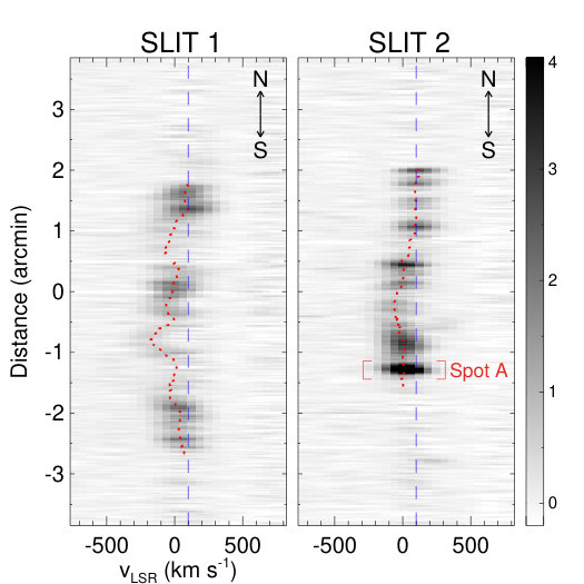 Figure 10
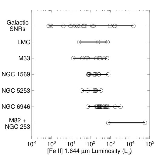 Figure 11
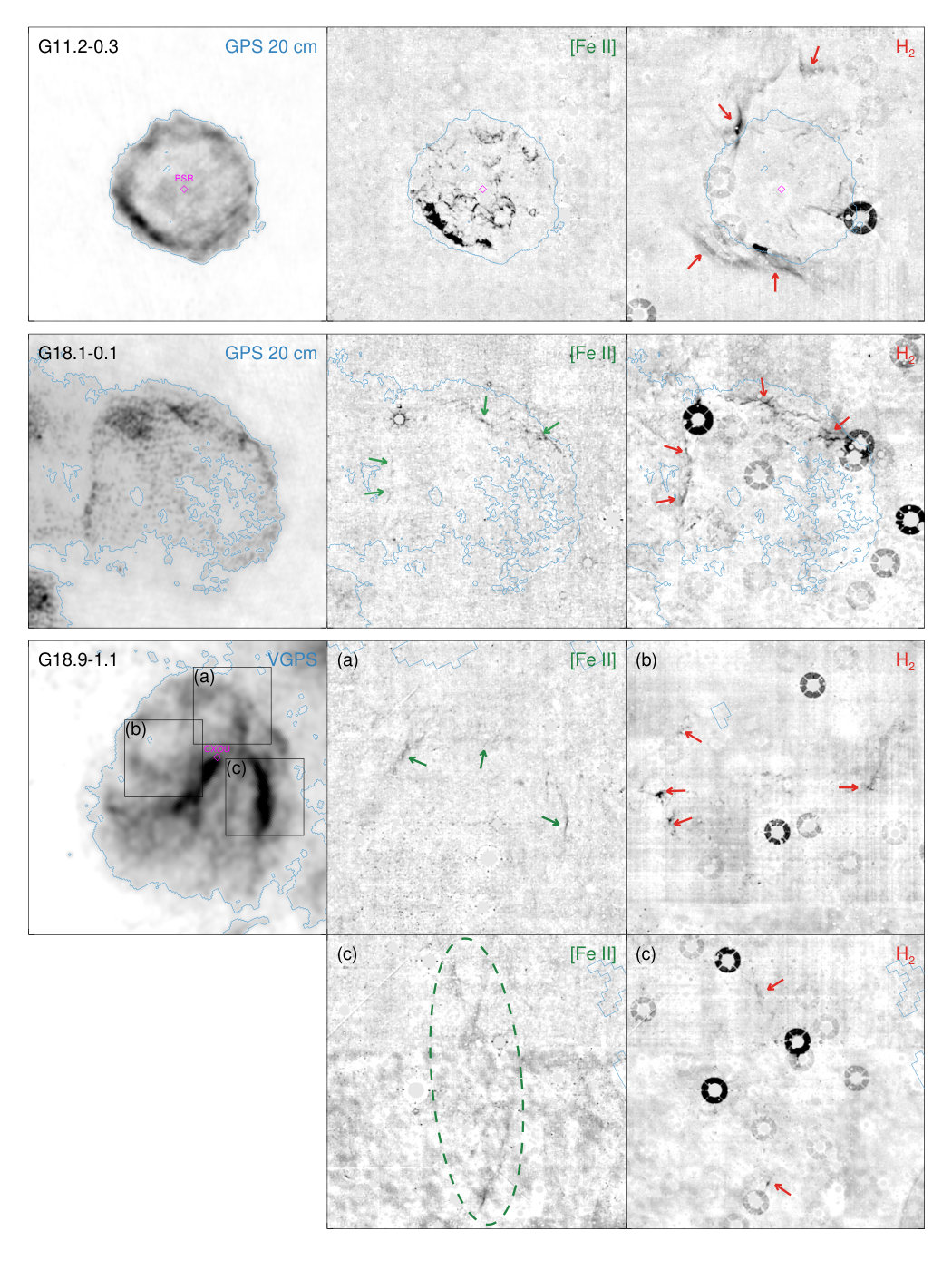 Figure 1
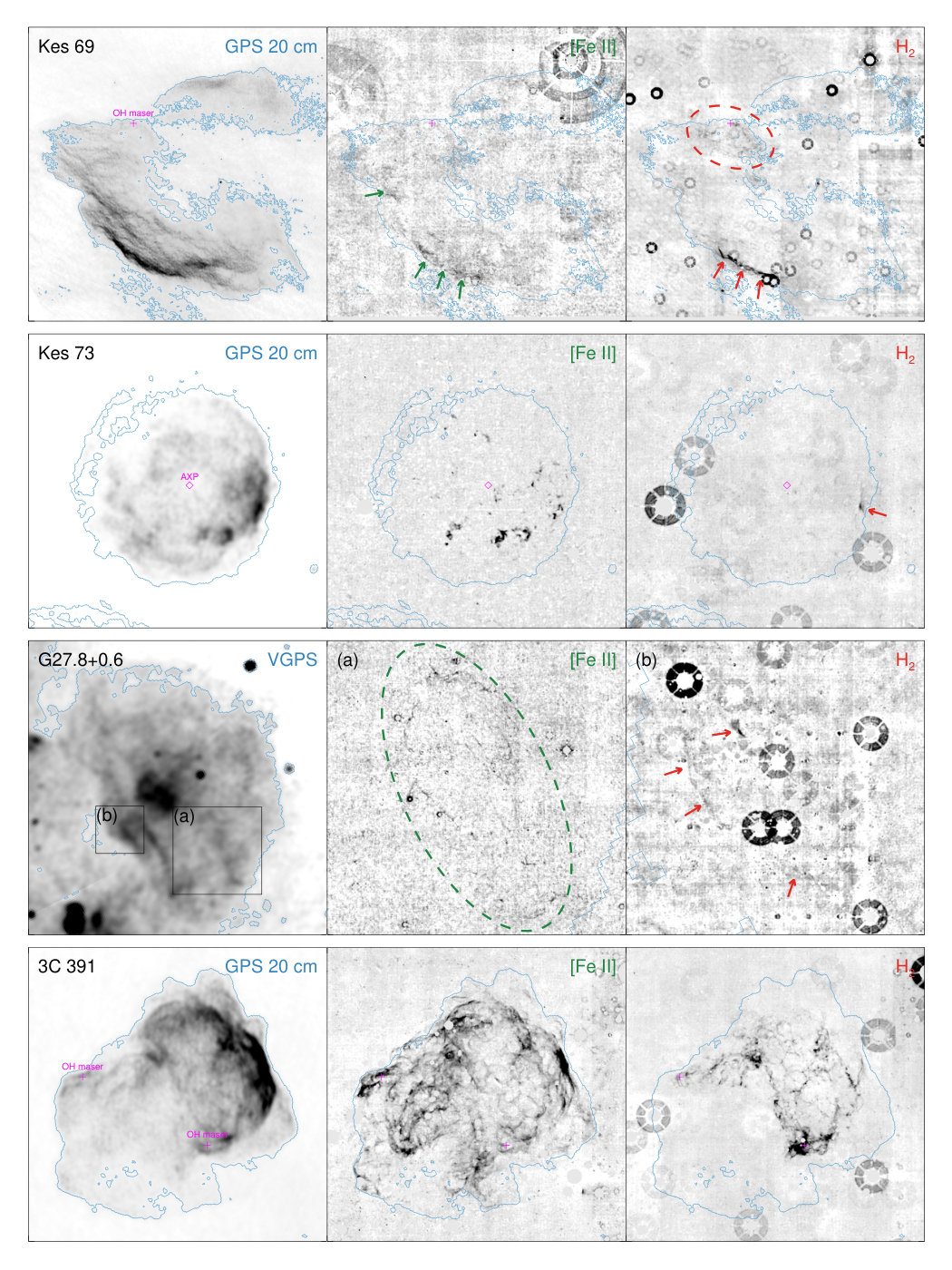 Figure 1
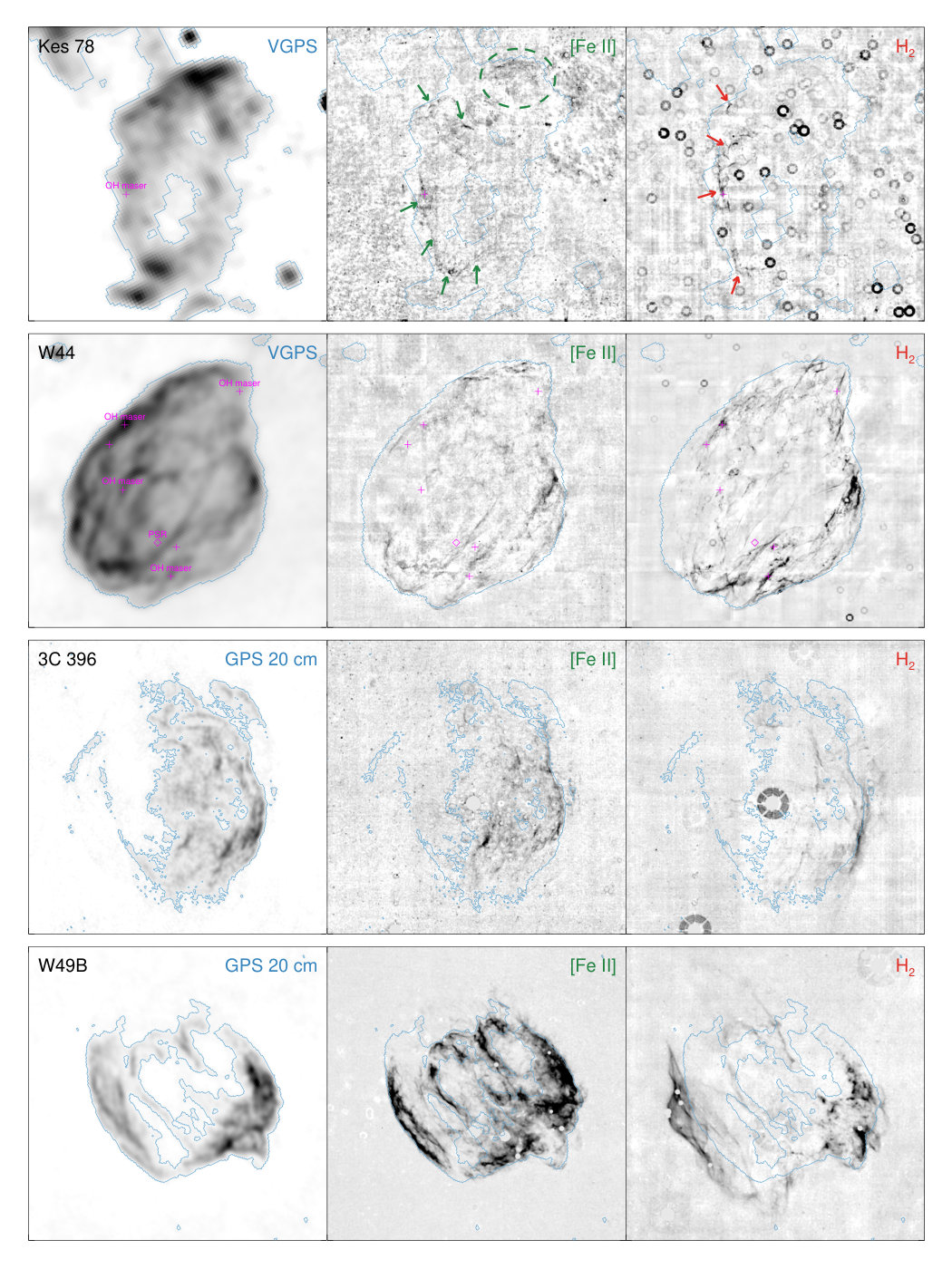 Figure 1
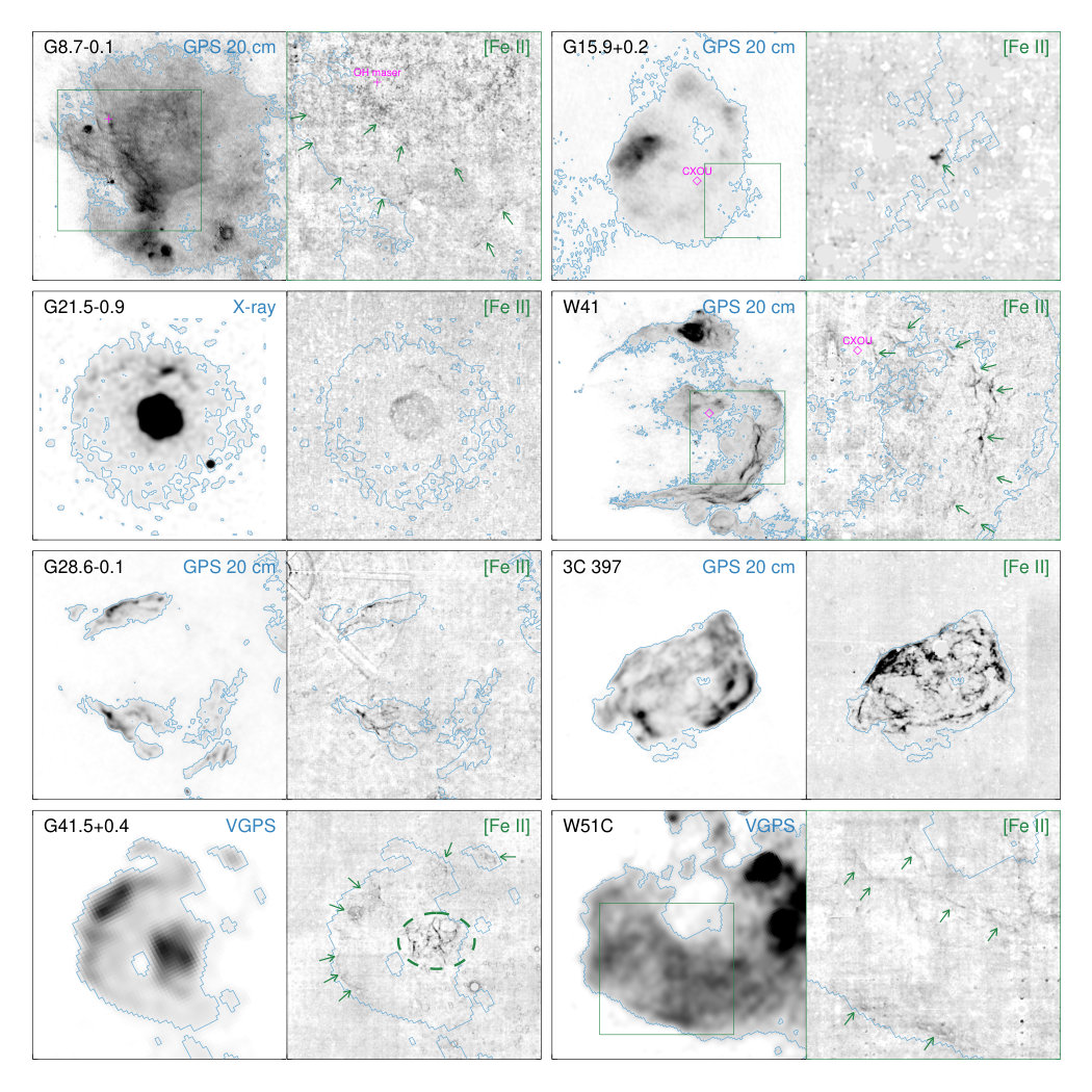 Figure 2
 Figure 3
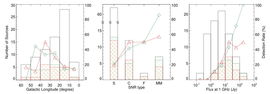 Figure 4
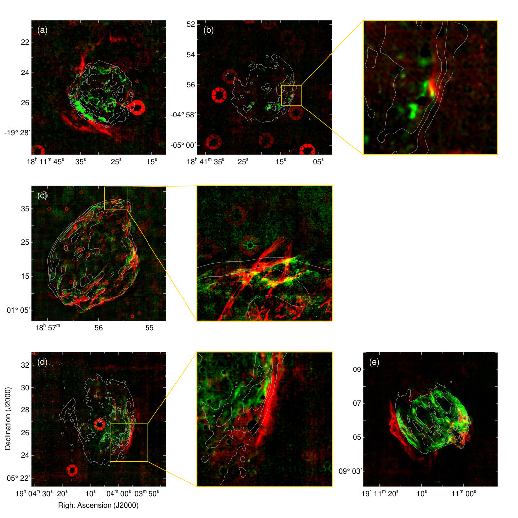 Figure 5
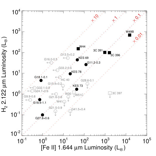 Figure 6
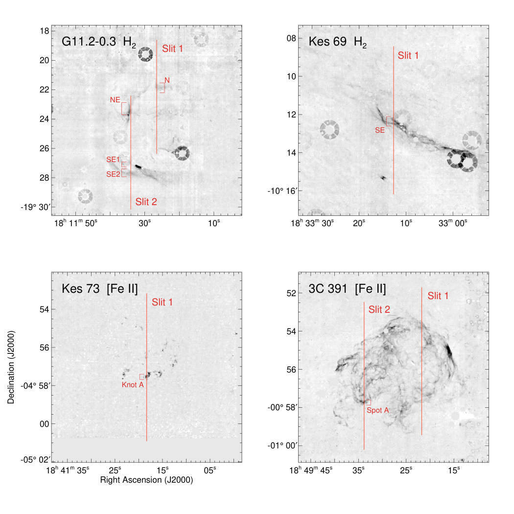 Figure 7
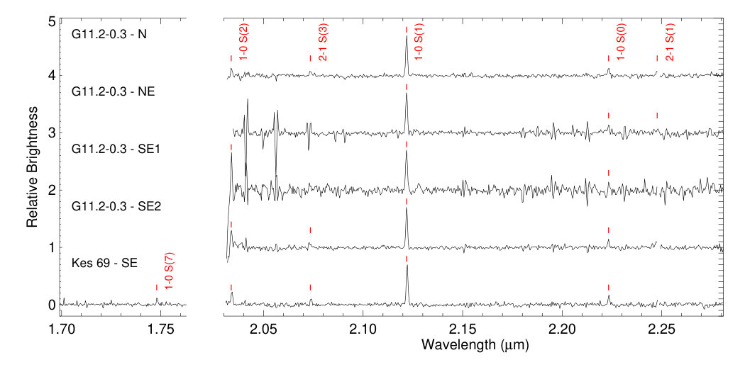 Figure 8
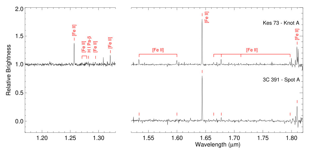 Figure 9
| Filter | BWaa Equivalent band width defined by , where is the maximum throughput of the filter response function (). | bb Mean wavelength of the filter defined by . | cc Zero-point level for the Vega continuum. It is described by , where is the spectral energy distribution of Vega (Rieke et al., 2008). denotes the “isophotal wavelength” at which the equals the flux density of the Vega continuum (see Tokunaga & Vacca (2005) and Rieke et al. (2008) for more information). | In-banddd Total in-band flux of the Vega spectrum falling in the passband, derived from the multiplied by the equivalent bandwidth (BW). | |
|---|---|---|---|---|---|
| (Å) | () | () | (W m-2 ) | (W m-2) | |
| [Fe II] | 284 | 1.645 | 1.666 | 1.15E-9 | 3.27E-11 |
| H2 | 211 | 2.122 | 2.122 | 4.66E-10 | 9.84E-12 |
| G-Name | Other Name | SizeaaSizes taken from Green’s SNR Catalog (Green, 2014). When it is asymmetric, the major and minor axes of the ellipse are given. | TypebbMorphological types of the SNRs in radio observations (Green, 2014). The “S,” “F,” and “C” represent “shell,” “filled-center,” and “composite” SNR type, respectively. The abbreviations within parentheses indicate mixed-morphology (MM) SNRs that display shell-like morphology in the radio but filled-center type in X-rays (Rho, 1995; Rho & Petre, 1998; Koo et al., 2016): Y (prototypical MM SNR), p (possible MM SNR). | ccFlux density at 1 GHz taken from Green’s SNR Catalog (Green, 2014). | Detection?ddDetection classifications in UWIFE and UWISH2 surveys: Y (detected), … (not detected). | |
|---|---|---|---|---|---|---|
| (arcmin) | (MM?) | (Jy) | [Fe II] | H2 | ||
| G | … | 12 | S | 2.8 | … | … |
| G | … | 5 4 | S | 1.2 | … | … |
| G | (W30) | 45 | S? | 80 | Y | … |
| G | … | 24 | S | 9 | … | … |
| G | … | 15 11 | S | 3.7 | … | … |
| G | … | 12 | S | 3.9 | … | … |
| G | … | 12 | S | 6.7 | … | Y |
| G | … | 6 | S | 0.9 | … | … |
| G | … | 11 9 | S | 1.3 | … | … |
| G | … | 18 12 | S | 5.8 | … | … |
| G | … | 11 7 | S | 1.0 | … | … |
| G | … | 12 10 | S | 2.3 | … | … |
| G | … | 4 | C | 22 | Y | Y |
| G | … | 8 | S? | 6 | … | … |
| G | … | 4 | S | 0.7 | … | … |
| G | … | 7? | ? | 3.5 | … | … |
| G | … | 6 5 | S | 0.8 | … | … |
| G | … | 6 5 | C? | 0.6 | … | … |
| G | … | 6 | S | 0.8 | … | … |
| G | … | 3 | C? | 0.8 | … | … |
| G | … | 5 4 | S | 3.5? | … | Y |
| G | … | 6 5 | S | 0.5 | … | … |
| G | … | 5 4 | S | 0.6 | … | … |
| G | … | 15 14 | S | 5.6 | … | … |
| G | … | 7 5 | S? | 5.0 | Y | … |
| G | … | 15 10 | S | 2.7 | … | Y |
| G | … | 13 | S | 4.6 | … | … |
| G | … | 4 | C | 3.0 | … | … |
| G | … | 5 | S | 0.5 | … | … |
| G | … | 6 | S | 0.4 | … | … |
| G | … | 8 | S | 4.6 | Y | Y |
| G | … | 6 | S | 1.4 | … | … |
| G | Kes 67 | 17 11 | S | 33 | … | … |
| G | … | 33 | C? | 37 | Y | Y |
| G | … | 27 | S | 10 | … | … |
| G | … | 10 | F | 10 | … | … |
| G | … | 8 | S? | 9? | … | … |
| G | … | 9 7 | S | 1.1 | … | … |
| G | … | 5 | C | 7 | Y | … |
| G | … | 5 | S | 0.4 | … | … |
| G | … | 13 | S | 1.4 | … | Y |
| G | Kes 69 | 20 | S | 65 | Y | Y |
| G | … | 26 | S? | 33 | … | … |
| G | W41 | 27 | S | 70 | Y | … |
| G | … | 10? | ? | 8? | … | … |
| G | … | 15? | S? | 8 | … | … |
| G | … | 30 15 | C? | 20? | … | Y |
| G | Kes 73 | 4 | S | 6 | Y | Y |
| G | … | 50 30 | F | 30 | Y | Y |
| G | … | 13 9 | S | 3? | Y | … |
| G | … | 5 | S | 1.5? | … | … |
| G | Kes 75 | 3 | C | 10 | … | … |
| G | … | 24 18 | S? | 6 | … | … |
| G | … | 18? | S? | 2? | … | … |
| G | 3C 391 | 7 5 | S (Y) | 25 | Y | Y |
| G | … | 40? | C? | ? | … | Y |
| G | … | 6 | S | 0.25? | … | … |
| G | Kes 78 | 17 | S? | 11? | Y | Y |
| G | … | 18 | S | 3.5 | … | Y |
| G | Kes 79 | 10 | S (Y) | 20 | … | … |
| G | W44 | 35 27 | C (Y) | 250 | Y | Y |
| G | … | 15 11 | S? | 9 | … | … |
| G | … | 25? | S? | 1.0 | … | … |
| G | 3C 396 | 8 6 | C (Y) | 18 | Y | Y |
| G | … | 22 | S | 11 | … | … |
| G | 3C 397 | 4.5 2.5 | S (Y) | 25 | Y | … |
| G | … | 10 | S? | 1? | Y | … |
| G | … | 8 | S? | 0.5? | … | … |
| G | … | 24 | S | 3? | … | … |
| G | W49B | 4 3 | S (Y) | 38 | Y | Y |
| G | … | 22 | S | 4.2? | … | … |
| G | (HC 30) | 17 13 | S | 17 | … | … |
| G | W51C | 30 | S? (p) | 160? | Y | … |
| G | … | 12? | C? | 0.5 | … | … |
| G | (HC 40) | 40 | S | 28 | … | Y |
| G | … | 20 15? | S | 0.5? | … | … |
| G | (4C 21.53) | 12? | S? | 1.8 | … | … |
| G | … | 15 | S | 3? | … | … |
| G | … | 20 16? | ? | 1.5 | … | … |
| Target | Slit Number | Slit Position | Filter | Exposure Time |
|---|---|---|---|---|
| [ (J2000) (J2000) ] | (s) | |||
| G11.20.3 | Slit 1 | 18:11:26.5 19:22:29 | ||
| Slit 2 | 18:11:34.0 19:26:17 | |||
| Kes 69 | Slit 1 | 18:33:12.6 10:12:18 | , | |
| Kes 73 | Slit 1 | 18:41:18.3 04:57:02 | , | |
| 3C 391 | Slit 1 | 18:49:21.7 00:55:34 | ||
| Slit 2 | 18:49:33.8 00:56:20 |
| G-Name | Other Name | Type | Distance | aaDetected [Fe II] 1.644 µm and/or \hh 2.122 µm fluxes. The uncertainty given by the quadrature sum of photometric uncertainty (6% for [Fe II] and 4% for \hh) and background RMS noise is less than 10% of the flux (see the text). | aaDetected [Fe II] 1.644 µm and/or \hh 2.122 µm fluxes. The uncertainty given by the quadrature sum of photometric uncertainty (6% for [Fe II] and 4% for \hh) and background RMS noise is less than 10% of the flux (see the text). | bb[Fe II] 1.644 µm and/or \hh 2.122 µm luminosities after correcting for extinction estimated from . | bb[Fe II] 1.644 µm and/or \hh 2.122 µm luminosities after correcting for extinction estimated from . | ReferenceccReferences of the adopted distances (fourth column) and column densities (fifth column). | |
|---|---|---|---|---|---|---|---|---|---|
| (MM?) | (kpc) | ( cm-2) | () | () | |||||
| G | (W30) | S? | 4.5 | 1.2 | 9.1 | … | 17 | … | 1 |
| G | … | S | 4.0 | 1.3eeColumn density estimated from the mean ratio of visual extinction to path length, mag kpc-1 (Whittet, 1992). | … | 0.48 | … | 0.52 | 2 |
| G | … | C | 4.4 | 3.0 | 13 | 7.4 | 120 | 26 | 3,4,5 |
| G | … | S | 13ddDistance derived from the relation. | 4.4eeColumn density estimated from the mean ratio of visual extinction to path length, mag kpc-1 (Whittet, 1992). | … | 0.76 | … | 54 | 6 |
| G | … | S? | 10ddDistance derived from the relation. | 4.0 | 0.082 | … | 9.4 | … | 6,7 |
| G | … | S | 7.5ddDistance derived from the relation. | 2.5eeColumn density estimated from the mean ratio of visual extinction to path length, mag kpc-1 (Whittet, 1992). | … | 4.1 | … | 32 | 6 |
| G | … | S | 5.6 | 1.8 | 0.17 | 1.6 | 0.83 | 4.5 | 8 |
| G | … | C? | 2.0 | 1.0 | 2.3 | 2.4 | 0.72 | 0.54 | 9,10 |
| G | … | C | 4.6 | 2.2 | 0.86 | … | 4.1 | … | 3,11 |
| G | … | S | 8.2ddDistance derived from the relation. | 2.8eeColumn density estimated from the mean ratio of visual extinction to path length, mag kpc-1 (Whittet, 1992). | … | 0.096 | … | 1.0 | 6 |
| G | Kes 69 | S | 5.2 | 2.4 | 6.3 | 13 | 46 | 44 | 12,13 |
| G | W41 | S | 4.2 | 1.4eeColumn density estimated from the mean ratio of visual extinction to path length, mag kpc-1 (Whittet, 1992). | 5.9 | … | 11 | … | 14 |
| G | … | C? | 3.5 | 1.2eeColumn density estimated from the mean ratio of visual extinction to path length, mag kpc-1 (Whittet, 1992). | … | 1.8 | … | 1.4 | 15 |
| G | Kes 73 | S | 8.5 | 2.6 | 1.8 | 0.16 | 43 | 1.7 | 16,17 |
| G | … | F | 2.0 | 1.5 | 2.0 | 0.33 | 0.98 | 0.10 | 18,19 |
| G | … | S | 9.6 | 3.5 | 2.1 | … | 140 | … | 20,21 |
| G | 3C 391 | S(Y) | 7.1 | 2.9 | 45 | 11 | 960 | 100 | 22,23 |
| G | … | C? | 4.6 | 0.2 | … | 2.8 | … | 2.0 | 24 |
| G | Kes 78 | S? | 4.8 | 0.7 | 15 | 8.6 | 21 | 9.4 | 25,26 |
| G | … | S | 7.9ddDistance derived from the relation. | 2.7eeColumn density estimated from the mean ratio of visual extinction to path length, mag kpc-1 (Whittet, 1992). | … | 1.4 | … | 14 | 6,27 |
| G | W44 | C(Y) | 2.8 | 1.7 | 45 | 220 | 51 | 150 | 3,28,29 |
| G | 3C 396 | C(Y) | 8.5 | 4.7 | 10 | 2.7 | 1600 | 97 | 30,31,32 |
| G | 3C 397 | S(Y) | 10 | 3.6 | 21 | … | 1700 | … | 33,34,35 |
| G | … | S? | 4.1 | 1.4eeColumn density estimated from the mean ratio of visual extinction to path length, mag kpc-1 (Whittet, 1992). | 12 | … | 21 | … | 20 |
| G | W49B | S(Y) | 10 | 5.0 | 53 | 11 | 15000 | 680 | 36,37,38 |
| G | W51C | S?(p) | 6.0 | 1.8 | 5.6 | … | 32 | … | 39,40,41 |
| G | (HC 40) | S | 6.6 | 2.5 | … | 1.1 | … | 6.4 | 22,42 |
| Wavelength | Identification | Relative FluxaaExtinction-corrected fluxes normalized by the H2 1–0 S(1) line assuming cm-2 for G11.20.3 (Lee et al., 2013; Borkowski et al., 2016) and cm-2 for Kes 69 (Yusef-Zadeh et al., 2003), and the extinction model of the general interstellar dust (Draine, 2003). The symbol “…” indicates that the lines are located outside of the spectral coverage or detector gap (for \hh 2–1 S(1)). We also mark with an * the lines that are contaminated by strong OH airglow emission lines such that we cannot measure their fluxes. | ||||
|---|---|---|---|---|---|---|
| (µm) | G11.20.3-N | G11.20.3-NE | G11.20.3-SE1 | G11.20.3-SE2 | Kes 69-SE | |
| 1.7480 | H2 1–0 S(7) | … | … | … | … | 0.23 (0.04) |
| 2.0338 | H2 1–0 S(2) | 0.27 (0.07) | … | bb upper limits for the undetected emission line. | 0.49 (0.13) | 0.28 (0.05) |
| 2.0735 | H2 2–1 S(3) | 0.17 (0.03) | * | * | 0.23 (0.06) | 0.16 (0.04) |
| 2.1218 | H2 1–0 S(1) | 1.00 (0.03) | 1.00 (0.05) | 1.00 (0.06) | 1.00 (0.03) | 1.00 (0.03) |
| 2.2233 | H2 1–0 S(0) | 0.19 (0.03) | 0.20 (0.08) | bb upper limits for the undetected emission line. | 0.17 (0.05) | 0.20 (0.03) |
| 2.2477 | H2 2–1 S(1) | 0.09 (0.05) | bb upper limits for the undetected emission line. | … | … | … |
| ccRadial velocity of the \hh 1–0 S(1) line at the local standard-of-rest frame. The uncertainty in parentheses is the statistical error by a single Gaussian fitting and does not include the wavelength-calibration error, which is roughly . () | (2) | (3) | (3) | (1) | (1) | |
| FWHMddFWHM of the \hh 1–0 S(1) line. The instrumental profile at has an FWHM of . () | (4) | (6) | (6) | (3) | (3) | |
| Wavelength | Identification | Relative FluxaaExtinction-corrected fluxes normalized by the [Fe II] 1.644 µm line assuming cm-2 for Kes 73 (Kumar et al., 2014) and cm-2 for 3C 391 (Sato et al., 2014), and the extinction model of the general interstellar dust (Draine, 2003). The symbol “…” indicates that the lines are located outside of the spectral coverage. | |
|---|---|---|---|
| (µm) | (lower–upper) | Kes 73-Knot A | 3C 391-Spot A |
| 1.1886 | [P II] - | bb upper limits for the undetected emission line. | … |
| 1.2570 | [Fe II] - | 1.42 (0.05) | … |
| 1.2707 | [Fe II] - | 0.08 (0.04) | … |
| 1.2791 | [Fe II] - | 0.17 (0.06) | … |
| 1.2822 | H I Pa | 0.12 (0.04) | … |
| 1.2946 | [Fe II] - | 0.14 (0.05) | … |
| 1.3209 | [Fe II] - | 0.38 (0.06) | … |
| 1.5339 | [Fe II] - | 0.17 (0.02) | 0.08 (0.02) |
| 1.5999 | [Fe II] - | 0.10 (0.01) | 0.04 (0.02) |
| 1.6440 | [Fe II] - | 1.00 (0.02) | 1.00 (0.02) |
| 1.6642 | [Fe II] - | 0.05 (0.01) | 0.02 (0.01) |
| 1.6773 | [Fe II] - | 0.11 (0.01) | 0.06 (0.01) |
| 1.7116 | [Fe II] - | 0.02 (0.01) | bb upper limits for the undetected emission line. |
| 1.7976 | [Fe II] - | 0.04 (0.01) | 0.03 (0.01) |
| 1.8099 | [Fe II] - | 0.26 (0.05) | 0.25 (0.04) |
| ccRadial velocity of the [Fe II] 1.644 µm line at the local standard-of-rest frame. The uncertainty in parentheses is the statistical error by a single Gaussian fitting and does not include the wavelength-calibration error, which is roughly . () | (1) | (1) | |
| FWHMddFWHM of the [Fe II] 1.644 µm line. The instrumental profile at has an FWHM of . () | (2) | (2) | |
Peer Reviews
No public reviews on file for this paper yet. If you reviewed it on a platform where reviews are public (OpenReview, ICLR, NeurIPS, ICML), you can paste yours below so the community can read it here.
Videos
No videos yet. Explain this paper in a talk, walkthrough, or lecture? Add one.
Near-infrared \feii and \hh Emission-line Study of
Galactic Supernova Remnants in the First Quadrant
Yong-Hyun Lee11affiliation: Department of Physics and Astronomy, Seoul National University, Seoul 151-742, Republic of Korea , Bon-Chul Koo11affiliation: Department of Physics and Astronomy, Seoul National University, Seoul 151-742, Republic of Korea , Jae-Joon Lee22affiliation: Korea Astronomy and Space Science Institute, Daejeon 305-348, Republic of Korea , Michael G. Burton33affiliation: School of Physics, University of New South Wales, Sydney, NSW 2052, Australia 44affiliation: Armagh Observatory and Planetarium, College Hill, Armagh, BT61 9DG, Northern Ireland, UK , and Stuart Ryder55affiliation: Australian Astronomical Observatory, P.O. Box 915, North Ryde, NSW 1670, Australia 66affiliation: Department of Physics and Astronomy, Macquarie University, Sydney, NSW 2109, Australia
Abstract
We report the detection of near-infrared (NIR) \feii (1.644 µm) and \hh 1–0 S(1) (2.122 µm) line features associated with Galactic supernova remnants (SNRs) in the first quadrant using two narrowband imaging surveys, UWIFE and UWISH2. Among the total of 79 SNRs fully covered by both surveys, we found 19 \feii-emitting and 19 \hh-emitting SNRs, giving a detection rate of 24% for each. Eleven SNRs show both emission features. The detection rate of \feii and \hh peaks at the Galactic longitude () of 40°–50° and 30°–40°, respectively, and gradually decreases toward smaller/larger . Five out of the eleven SNRs emitting both emission lines clearly show an “\feii–\hh reversal,” where \hh emission features are found outside the SNR boundary in \feii emission. Our NIR spectroscopy shows that the \hh emission originates from collisionally excited \hh gas. The brightest SNR in both \feii and \hh emissions is W49B, contributing more than 70% and 50% of the total \feii 1.644 µm () and \hh 2.122 µm () luminosities of the detected SNRs. The total \feii 1.644 µm luminosity of our Galaxy is a few times smaller than that expected from the SN rate using the correlation found in nearby starburst galaxies. We discuss possible explanations for this.
infrared: ISM — ISM: clouds — ISM: supernova remnants — surveys
1 Introduction
In our Galaxy, there are about 300 known supernova remnants (SNRs; Green, 2014). They show diverse morphology and properties, which are either inherited from the supernova (SN) explosion or acquired through the interaction with their ambient medium. For massive core-collapse SNRs, the ambient medium could be the circumstellar medium (CSM) that their progenitor stars ejected, or the interstellar medium (ISM) shaped by the progenitors through their stellar winds and/or ultraviolet (UV) photons, or even the molecular clouds (MCs) from which their progenitors had formed. Therefore, knowing the environment is not only essential for understanding the morphology and evolution of SNRs, but is also helpful for exploring the connection among SNRs, SNe, and progenitor stars.
A useful tool to study the SNR environment and the interaction of SNRs with it is the near-infrared (NIR; 1–5 µm) waveband. Most SNRs are located in the Galactic plane where the interstellar extinction is large, so the NIR waveband has a great advantage over the optical waveband. In the NIR waveband, there are two prominent lines tracing shocks propagating into dense media: (1) the 1.644 µm (; also 1.257 µm from ) forbidden line of single ionized Fe (\feii) and (2) the 2.122 µm ( = 1–0 S(1)) line of molecular hydrogen (\hh). The \feii lines trace radiative, fast (–) -type shocks. In radiative -type shocks propagating through either atomic or molecular gas, an extended region of partially ionized gas at constant temperature (6000–8000 K) is developed in the postshock relaxation layer (Shull & McKee, 1979; Hollenbach & McKee, 1989; Koo et al., 2016, and references therein). In this temperature plateau region, where the gas is photoionized by the strong UV radiation generated from the hot gas just behind the shock front, Fe is mainly in Fe*+* and the electron density is high. Hence, the NIR \feii lines, having excitation temperatures of K, can be easily excited. In SNRs, \feii 1.644 µm and 1.257 µm lines are indeed much stronger than H recombination lines (e.g., Oliva et al., 1989; Mouri et al., 2000; Koo & Lee, 2015). The \hh 2.122 µm line mainly traces slow () nondissociative -type shocks (Draine, 1980; Chernoff et al., 1982; Draine & Roberge, 1982). In -type shocks propagating through molecular gas of low fractional ionization, the temperature of the shocked gas is K and \hh is not dissociated, so that strong \hh lines from rovibrational transitions are emitted in the NIR waveband. In principle, \hh lines can also be emitted from dissociative -type shocks if the shock has swept up enough column density, i.e., cm*-2*, and \hh molecules are re-formed (Hollenbach & McKee, 1979, 1989; Neufeld & Dalgarno, 1989). Another important excitation mechanism of \hh is absorption of far-UV photons (– eV). The radiative cascade of the excited \hh downward to the ground state also produces strong \hh lines (e.g., Black & Dalgarno, 1976; Black & van Dishoeck, 1987). Because the shocked hot plasma is a strong UV and X-ray emitter, we might also expect \hh lines excited by UV fluorescence around the remnant.
NIR \feii and \hh emission lines have been studied extensively in several bright Galactic SNRs: Kepler (Oliva et al., 1989; Gerardy & Fesen, 2001), G11.20.3 (Koo et al., 2007; Moon et al., 2009), 3C 391 (Reach et al., 2002), W44 (Reach et al., 2005), 3C 396 (Lee et al., 2009), W49B (Keohane et al., 2007), Cygnus loop (Graham et al., 1991), Cassiopeia A (Gerardy & Fesen, 2001; Lee et al., 2017; Koo et al., 2018), Crab nebula (Graham et al., 1990; Loh et al., 2011), IC 443 (Treffers, 1979; Graham et al., 1987; Burton et al., 1988, 1990; Kokusho et al., 2013), MSH 15-52 (Seward et al., 1983), RCW 103 (Oliva et al., 1990; Burton & Spyromilio, 1993). According to these studies, SNRs bright in \feii emission lines may be divided into two groups (Koo, 2014): (1) young SNRs interacting with their dense CSMs (e.g., G11.20.3, W49B, Cassiopeia A) and (2) middle-aged SNRs interacting with dense atomic gas or MCs (e.g., IC 443, W44). In young core-collapse SNRs, such as Cassiopeia A and G11.20.2, strong \feii emission from shocked SN ejecta, with very high expansion velocities (), has also been detected (Gerardy & Fesen, 2001; Moon et al., 2009; Koo et al., 2013; Lee et al., 2017). The \hh emission, on the other hand, arises from slow, nondissociative -type shocks, so that it has been observed mainly from middle-aged SNRs interacting with MCs. In some SNRs, e.g., G11.20.3, 3C 391, W44, 3C 396, W49B, IC 443, and RCW 103, both \feii and \hh lines have been detected, indicating a complex structure of the ambient medium.
The observed NIR \feii and \hh emission lines around SNRs are thought to be mostly produced in SNR shocks, which could be either fast -type and slow -type depending on the SNR properties and environment. But for some SNRs, their excitation mechanism as well as their nature are uncertain. A long-standing problem is to explain the extended \hh emission features observed outside the \feii/radio/X-ray boundary of several Galactic SNRs: G11.20.3 (Koo et al., 2007), 3C 396 (Lee et al., 2009), W49B (Keohane et al., 2007), Cygnus loop (Graham et al., 1991), and RCW 103 (Oliva et al., 1990; Burton & Spyromilio, 1993). If the shocks are driven by the same SN blast wave, we expect the \hh filaments to be closer than the \feii filaments to the explosion center, because in general the former is from slower -type shocks whereas the latter is from fast -type shocks. Therefore, this “\feii–\hh reversal” feature observed in SNRs requires an explanation. Several explanations have been proposed, e.g., UV fluorescence excitation, X-ray heating, magnetic precursor, reflected shock, and complex projection effect (e.g., Oliva et al., 1990; Graham et al., 1991; Burton & Spyromilio, 1993; Keohane et al., 2007; Koo et al., 2007; Lee et al., 2009), but the feature remains poorly understood.
Because the two NIR emission lines are closely associated with SNR shocks, we expect some connection between the characteristics of these lines and SN activity in galaxies (e.g., Greenhouse et al., 1991). In particular, because NIR \feii emission lines are bright in SNRs but faint in H II regions, we expect a correlation between the \feii luminosity and the SN rate of a galaxy (Graham et al., 1987; Koo & Lee, 2015, and references therein). Indeed, some studies have shown a strong correlation between \feii 1.257/1.644 µm luminosity and SN rates in bright external galaxies, (e.g., Morel et al., 2002; Alonso-Herrero et al., 2003; Rosenberg et al., 2012). However, in nearby galaxies where we can resolve individual SNRs, it is found that about 70–80% of the \feii flux arises from diffuse emission of unknown origin and that only a small fraction of the SNRs are bright in \feii emission (Alonso-Herrero et al., 2003). In order to better understand the relation between \feii luminosity and SN rate, therefore, we need to understand the origin of the diffuse \feii emission and the population of \feii-bright SNRs.
In this paper, we carry out a systematic study of SNRs using two recent \feii and \hh narrowband imaging surveys covering the first quadrant of our Galaxy (Froebrich et al., 2011; Lee et al., 2014). Using these systematic and unbiased NIR emission surveys, together with NIR spectroscopic observations, we investigate the environment and nature of the SNRs. This paper is organized as follows. In Section 2, we outline the NIR imaging and spectroscopic observations and their data reduction/analysis. The results from the imaging surveys are presented in Section 3 together with the spectroscopic results for four Galactic SNRs. We discuss the environment and nature of the SNRs in Section 4, and the summary of this paper is given in Section 5.
2 Observations and Data Analysis
2.1 Near-infrared Narrowband Imaging Surveys
2.1.1 Brief description of the surveys
The \feii and \hh narrowband imaging surveys that constitute UWIFE and UWISH2 were carried out with the Wide-Field Camera (WFCAM) at the United Kingdom Infrared Telescope (Froebrich et al., 2011; Lee et al., 2014). The WFCAM consists of four separated Rockwell Hawaii-II detectors with a pixel scale of and each detector spaced 94% of the imaging area apart (Casali et al., 2007). The basic observing unit of a single WFCAM tile is composed of a macrostepping sequence in order to fill this spacing, so that the tile covers a continuous field of view of 0.75 square degrees. An additional microstepping sequence with an interlacing technique has been used during the entire surveys in order to prevent undersampling at good seeing conditions (less than 08). Therefore, the final stacked images provide pixel sampling. The single exposure time per frame is 60 s, but the microstepping and three jittering observations result in a total integration time per pixel () of 720 s. The \feii narrowband filter used in the UWIFE survey has a mean wavelength () of and a bandwidth () of 284 Å, while the \hh 1–0 S(1) narrowband filter used in the UWISH2 survey has and 211 Å. The detailed descriptions for both filters are listed in Table 1. Both surveys fully cover the first Galactic quadrant of and . The median seeing of the UWIFE and UWISH2 surveys is and , respectively, and the typical rms noise level of both surveys goes down to (1.4–1.6) in the unbinned image with a pixel scale. More detailed information is provided in Lee et al. (2014) for the UWIFE survey and Froebrich et al. (2011) for the UWISH2 survey.
2.1.2 Data Reduction and Continuum Subtraction
All WFCAM data are preprocessed by the Cambridge Astronomical Survey Unit and are distributed through a dedicated archive hosted by the Wide Field Astronomy Unit. During the process, astrometric and photometric calibration have been made with the Two Micron All Sky Survey (2MASS) point-source catalog (Skrutskie et al., 2006). A detailed description of the process is presented in Dye et al. (2006).
To search for extended \feii/\hh emission features more efficiently, we performed continuum-subtraction using the broad H-/K-band images obtained as part of the UKIDSS GPS (Lucas et al., 2008). We first smoothed whichever image was observed in the better seeing in order to match their point-spread functions (PSFs), after which the broadband image was scaled to match their fluxes. In order to suppress the residuals from bright stars as much as possible, we performed PSF-fitting photometry by using an empirical PSF model constructed from well-sampled, bright reference stars. For this, we utilized StarFinder, an IDL-based code for deep analysis of stellar fields (Diolaiti et al., 2000). Then, bright stars in both narrow- and broadband images are removed using flux-scaled PSF models. The final continuum-subtracted \feii/\hh images are obtained from image-to-image subtraction of the “bright point source removed” narrow- and broadband images. The detailed processing steps of this continuum-subtraction is described further in Section 3.3 of Lee et al. (2014).
2.1.3 Identification and Flux Measurement
Among the 294 known Galactic SNRs (Green, 2014), 79 SNRs are fully covered by both surveys and are listed in Table 2. From the continuum-subtracted images, we identified \feii and \hh emission features around the SNRs by eye. We found various morphologies of the emission lines that seem to be associated with the SNRs. We also cross-checked our results with published catalogs, which were obtained by an automated code (Froebrich et al., 2015). They reported the detection of \hh lines toward 30 Galactic SNRs, 11 of which are either partially covered in the UWIFE survey or outside of the UWIFE survey area.
In order to measure the fluxes of the identified emission features using the continuum-subtracted images, we first performed median-filtering with a “window” size of 10 pixels and masked the star residuals around saturated stars with -/-band magnitudes of mag using the 2MASS catalog to prevent artifacts from dominating the total fluxes (e.g., hot pixels from cosmic-ray hits, residuals around a saturated star, etc.; see Froebrich et al. 2015 for details). We then measured the fluxes with an appropriate circular or elliptical aperture encircling the emission features. The local background level was estimated from an annulus with a radius 1.2–1.5 times larger than the source region. The total flux () of \feii and \hh line emission is derived from
[TABLE]
where is the total in-band flux of each narrowband filter for Vega (see Table 1), DN is the total digital number of the target during a 60 s exposure time, and is the effective exposure time fixed to 60 s. is a zero-point magnitude of the target image corresponding to the magnitude at , which is established by comparing the bright, isolated stars in the field with the 2MASS -/-band point-source catalog. The uncertainty of the total flux is derived from the quadrature sum of (1) the absolute calibration uncertainty and (2) the standard deviation of the background variation. Since the background level around the source is quite stable, most of the flux error arises from the calibration uncertainty. The typical calibration error, derived from the uncertainty of the zero-point magnitude over the survey data, is 0.06 mag for UWIFE and 0.04 mag for UWISH2, corresponding to 6% and 4% of the total fluxes, respectively. Even in the worst cases, the total uncertainty does not exceed 10% of the total flux. The H- and K-band images used for the continuum-subtraction (see Section 2.1.2) include a small portion of \feii and \hh emission lines, so the flux measured from the continuum-subtracted image is roughly 10% smaller than the true \feii/\hh flux, corresponding to the bandwidth ratios of the narrowband and the broadband filters. In order to compensate for such “leakage of \feii/\hh flux,” we multiplied the derived \feii and \hh fluxes by a factor of 1.15 (\feii) and 1.10 (\hh), respectively. These two correction factors were derived from the assumption that the only emission line in the H band is the \feii 1.644 µm line and in the K band, the \hh 2.122 µm line.
2.2 Near-infrared Spectroscopy
We carried out long-slit NIR spectroscopic observations for four Galactic SNRs (G11.20.3, Kes 69, Kes 73, and 3C 391) in which the bright \feii and \hh emission lines are detected, in order to investigate their excitation mechanisms and origins. These observations were performed with the Infrared Imager and Spectrograph 2 (IRIS2; Tinney et al., 2004) on the 3.9 m Anglo-Australian Telescope, which provides a spectral resolution of 2200–2500 with a pixel scale of 045 per pixel in each of the , , and bands. The observations were done in 2012 April 7–8 for G11.20.3, and in 2011 June 27 for the other SNRs. The position angle of the slit is , i.e., from the north to south direction. All observations were performed with multiple on–off nodding sequences in order to remove night-sky airglow emission lines within the wavebands. The observation logs are listed in Table 3.
We followed the general data reduction procedure. First, all of the observed raw spectra were subtracted by the dark frame and then divided by a normalized flat frame. Using more than a dozen bright OH airglow emission lines, we derived the two-dimensional wavelength solution that gives a 1 uncertainty of 2–3Å over the wavelength coverage. The night-sky airglow emission lines together with thermal background continuum in the band was subtracted by the off-position frame. Finally, we performed photometric calibration by comparing the observed spectrum of an A0V type standard star with the Kurucz model spectrum111http://kurucz.harvard.edu/. The 1 uncertainty of the absolute flux calibration reaches up to 30% of its flux, due to centering of standard star observations; however, the relative uncertainty within each band is very robust.
3 Results
3.1 [Fe II]/H2 SNRs in the UWIFE and UWISH2 Surveys
3.1.1 Catalog and Some Statistics
Among the 79 SNRs covered by these surveys, we have identified 19 SNRs with \feii emission features in the UWIFE survey and 19 SNRs with \hh emission features in the UWISH2 survey. Eleven of them show both emission features. The identified SNRs are marked by “Y” in the last two columns of Table 2, and their \feii and/or \hh images are presented in Figures 1–3: SNRs with both \feii and \hh lines in Figure 1, SNRs with \feii lines only in Figure 2, and SNRs with \hh lines only in Figure 3. Among the 19 \feii-line-detected SNRs, six had been known from previous NIR imaging and spectroscopic observations: G11.20.3 (Koo et al., 2007), G21.50.9 (Zajczyk et al., 2012), 3C 391 (Reach et al., 2002), W44 (Reach et al., 2005), 3C 396 (Lee et al., 2009), and W49B (Keohane et al., 2007). The rest (13 out of 19; %) are newly discovered in our survey. Among the 19 \hh-emitting SNRs, five of them had been known from previous studies: G11.20.3 (Koo et al., 2007), 3C 391 (Reach et al., 2002), W44 (Reach et al., 2005), 3C 396 (Lee et al., 2009), and W49B (Keohane et al., 2007). The rest (14 out of 19; %) are new discoveries. The detection rate is 24% for each survey. For comparison, 30–50% of radio SNRs in M82 and NGC 253 are detected in \feii emission (Alonso-Herrero et al., 2003). The lower detection rate in the Milky Way might be partly due to the high interstellar extinction in the galactic disk. On the other hand, the high detection rate in external galaxies could be because the target SNRs are radio-bright ones. As we will see in the next paragraph, the radio-bright SNRs have high detection rates in \feii emission.
Figure 4 shows the \feii and \hh detection rates as a function of Galactic longitude, SNR type, and 1 GHz flux density. The distribution of the 79 SNRs falling in the survey area is shown by the black empty histogram, while those of the \feii- and \hh-emitting SNRs are presented as green and red hatched histograms, respectively. The detection rate in each bin is also overplotted as green diamonds and red triangles, respectively. In the left panel, we see that the distribution of the 79 SNRs peaks at longitude °–20° and gradually decreases toward high Galactic longitude. The small number in the bin at °–10° is due to the limited coverage of the survey (7°62°). The detection rate is below 20% at small and increases toward large , reaching a maximum of 50% at 40°–50° for the \feii line and at 30°–40° for the \hh line. It then decreases again to larger . The low detection rate at small might be due to the large interstellar extinction toward this direction, while the low detection rate at large could be due to the relatively diffuse environment there. The middle panel of the figure shows that most (62 out of 79) of the SNRs in the survey area are shell-type SNRs and that their \feii/\hh detection rate is . The detection rate for the composite SNRs is considerably higher than this, i.e., , while for the filled-centered SNRs, the small number limits statistics. Alongside the three radio morphological types, we also show the detection rate of the mixed-morphology (MM) SNRs. MM SNRs, which are also known as “thermal-composite” SNRs, show filled-centered thermal X-ray emission surrounded by radio shells, and most of them show evidence for interaction with MCs (Rho, 1995; Rho & Petre, 1998; Koo et al., 2016). There are six SNRs known to be MM types plus one MM SNR candidate in our survey area. (Five of them are shell type and two are composite type in radio.) The detection rate of MM SNRs is very high, i.e., % () in \feii and % () in \hh emission. The only MM SNR not detected in the \feii line is G33.60.1 (Kes 79), which is at a distance of 7.5 kpc (Giacani et al., 2009), so that the nondetection could be due to large extinction. The high detection rate of MM SNRs is consistent with the consensus that these SNRs are in dense environments (see Section 3.1.2). In the right panel of the figure, we see that the \feii- and/or \hh-emitting SNRs have relatively higher 1 GHz flux density, i.e., 1–300 Jy. Furthermore, the detection rates are gradually increasing with the 1 GHz flux density. Radio brightness is enhanced when SNRs interact with a dense environment, due to higher magnetic fields and/or higher relativistic electron densities. So, this apparent correlation could also be due to their dense environment.
3.1.2 Morphology and Luminosity
In most SNRs, \feii emission is confined to thin filaments or partial shell-like structures that are correlated well with bright radio continuum features. Prototypical SNRs are G28.60.1, 3C 391, W44, 3C 396, and W49B. Such morphology is consistent with the \feii emission arising from a postshock cooling region behind a radiative SNR shock propagating into the ambient medium. Some SNRs, however, show \feii emission that does not fit into this category: (1) G11.20.3 where arc-like \feii emission features are detected in the central area. Spectroscopic observations suggest that these \feii features are associated with fast-moving () SN ejecta (Moon et al., 2009). (2) G21.50.9 and G41.50.4, where the \feii emission associated with pulsar wind nebula (PWN) is detected. In G21.50.9, the \feii emission is confined to thin filaments surrounding the PWN. This \feii emission had been previously reported by Zajczyk et al. (2012). In G41.50.4, bright complex \feii filaments are detected on the central radio structure, which is thought to be a PWN (Kaplan et al., 2002). (3) Kes 73 and G15.90.2, where \feii emission features are clumpy not filamentary. In Kes 73, the \feii emission is distributed over the entire remnant along the radio-bright filaments, but it is confined to dozens of knotty clumps. In G15.90.2, a small () \feii clump without enhanced radio continuum emission is detected near the southwestern boundary of the remnant.
\hh
emission is also detected mainly toward the bright radio filament/shell in most SNRs. Although the \hh emission arises from slow, nondissociative -type shocks while the radio emission is synchrotron radiation, the dense environment might cause this correlation. In some SNRs, however, \hh emission has been detected beyond the SNR radio boundary. Prototypical SNRs are G11.20.3, Kes 73, W44, 3C 396, and W49B (see Figure 5; a small \hh filament is detected outside the western boundary of G21.60.8, too, but their association is not clear). In G11.20.3 and W49B, for example, we can see extended prominent \hh emission well beyond the SNR boundary. Note that in the aforementioned five SNRs \feii emission is also detected and the offset of \hh emission from the \feii emission is noticed (i.e., Koo et al. 2007 for G11.20.3; Keohane et al. 2007 for W49B, Lee et al. 2009 for 3C 396, and Koo 2014 for W44). As we mentioned in Section 1, this feature, i.e., \hh emission farther outside than the \feii emission, is known as the “\feii–\hh reversal” and needs an explanation. We will discuss this in Section 4.1.2.
The observed total \feii and \hh fluxes of the 27 SNRs are summarized in Table Near-infrared \feii and \hh Emission-line Study of Galactic Supernova Remnants in the First Quadrant. The table also lists the adopted distances and the resulting \feii 1.644 µm and \hh 2.122 µm luminosities. The extinction correction has been made by using the column densities () available in literature, assuming the general interstellar dust extinction model (Draine, 2003). The luminosity ranges are 0.72– for \feii and 0.52– for \hh. W49B is the brightest in either emission. The total \feii 1.644 µm luminosity is and W49B contributes more than 70% of the total \feii 1.644 µm luminosity. For comparison, the total \hh 2.122 µm luminosity is , half of which is attributed to W49B. The uncertainty in the measured flux is less than 10% (see Section 2.1.3), but the uncertainty of the derived luminosity could be very large, due to the uncertain distance (and uncertain column density). For example, the distance to W49B reported in previous studies varies from 8.0 to 12.5 kpc (Lockhart & Goss, 1978; Moffett & Reynolds, 1994; Zhu et al., 2014), and the hydrogen column density is in the range (4.8–5.3) cm*-2* (Hwang et al., 2000; Keohane et al., 2007). The \feii and \hh luminosities of W49B, therefore, are uncertain by a factor of 2.
Even though the two NIR emission lines arise from different types of shocks, their luminosities seem to be correlated. This is shown in Figure 6 where the filled symbols represent 11 SNRs detected in both \feii and \hh emission while the empty symbols represent the SNRs detected only in one emission line. MM SNRs are marked with squares. The correlation coefficient for the 11 SNRs is . The brightest SNRs, i.e., W49B, 3C 396, 3C 391, and W44, are MM SNRs interacting with a dense ambient medium. Among the six known MM SNRs in the survey area, 3C 397 and W51C are exceptions. 3C 397 is very bright in \feii but not detected in \hh, and its nature as an MM SNR is uncertain (Section 4.1.1). In W51C, only \feii emission is detected. Koo & Moon (1997) detected shocked CO but not shocked \hh, and concluded that the shock is a fast -type shock and that CO has been reformed but \hh has not been yet. The nondetection of \hh emission also suggests that no strong -type shocks are present in this SNR.
3.2 Spectroscopy of Four SNRs
We carried out NIR spectroscopic observations of four of the SNRs, i.e., G11.20.3, Kes 69, Kes 73, and 3C 391, showing both \feii and \hh emission features. Their enlarged \feii/\hh images, together with the slit positions, are shown in Figure 7. In the - and -band spectra of G11.20.3 and Kes 69, we detected \hh 1–0 S(1) at 2.122 µm and other relatively weak \hh lines associated with \hh filaments (Figure 8). In the - and -band spectra of Kes 73 and 3C 391, on the other hand, we detected the \feii 1.644 µm line and other weak \feii (+ Pa ) lines associated with \feii filaments (Figure 9). We performed a single Gaussian fitting for all of the detected lines to derive their line-of-sight velocities, line width, and fluxes. The derived line parameters are listed in Tables 5 and 6. In the following, we describe the results for individual sources.
For G11.20.3, we obtained -band spectra along two long slits crossing the extended \hh filaments. We obtained 1D spectra at four different positions: N, NE, SE1, and SE2 (Figure 8). The flux ratio of \hh 1–0 S(0) to 1–0 S(1) is in all filaments (Table 5), which is consistent with the collisionally excited \hh emission at a few 1000 K (; Black & van Dishoeck, 1987). Note that the ratio for UV fluorescence \hh ranges from 0.4 to 0.6, which is higher than that for collisional excitation (Black & van Dishoeck, 1987). Weak/no \hh lines from high vibrational levels with (2–1 S(3) at 2.07 µm and 2–1 S(1) at 2.25 µm) also support the collisional process of the \hh filaments. The of all \hh filaments extended over G11.20.3 is between and (Table 5), which agrees with the systematic velocity of the remnant (; Green et al., 1988). This implies that the \hh filaments are indeed physically associated with the remnant despite their large extension.
For Kes 69, we obtained - and -band spectra along a slit crossing the bright southeastern \hh filament. We detected bright \hh 1–0 S(1) and other weak \hh lines but no ionic lines were detected. There is some \feii emission seen in the image (Figure 1), but the sensitivity of the -band spectrum is very weak, and no \feii lines were detected. The ratio of \hh lines is again consistent with collisional excitation (Table 5). The of the \hh filaments is (Table 5). It is known that the SNR is interacting with adjacent MCs in this area (Zhou et al., 2009, and references therein). Zhou et al. (2009) proposed that an MC at is associated with the SNR. Therefore, there is a large difference (–) between the velocities of the CO and \hh emission. We can hypothesize two possible explanations. First, the CO emission traces the ambient MC, whereas the \hh emission is from the shocked \hh gas. Hence, the velocity difference may represent the shock velocity propagating into the MC. However, the \hh filaments are located in the outer boundary of the remnant, so the shock velocity along the line of sight might be almost negligible. Second, the systematic velocity of the SNR could be , not . It is not easy to find an MC associated with an SNR in the inner Galaxy, due to the confusion by foreground and background CO emission. Indeed, we see some CO emission at in the channel maps of Zhou et al. (2009). If the systemic velocity of the SNR is (Table 5), then assuming the flat Galactic rotation model with the IAU standard rotation constants ( kpc, ), the kinematic distance to Kes 69 would be kpc. This is considerably smaller than the previous estimation, e.g., 5.2–5.6 kpc (Tian & Leahy, 2008; Zhou et al., 2009; Ranasinghe & Leahy, 2018).
In Kes 73, one slit is centered on the brightest \feii clump (hereafter “Knot A”) in the central area. We have detected a dozen bright \feii lines and a weak Pa line in its - and -band spectra (Figure 9). The detection of the H recombination line, together with the nondetection of the [P II] 1.189 µm line, indicates that the knot is either shocked ambient medium or H-rich SN ejecta with cosmic P/Fe abundance (Koo et al., 2013; Lee et al., 2017). The observed central velocity of the line, however, is only . According to SN explosion models, the H-rich SN ejecta from the progenitor’s envelope show an expansion velocity of more than a few and no less than –, even in significant mixing among the nucleosynthetic layers (Kifonidis et al., 2006; Hammer et al., 2010; Wongwathanarat et al., 2015). Therefore, Knot A is probably not shocked SN ejecta but shocked ambient medium. Compared to the systematic velocity of the remnant ( to ) for Kes 73 (Tian & Leahy, 2008; Kilpatrick et al., 2016), however, it is much () larger, so that the shocked ambient medium might be the CSM not the ISM. This is consistent with the clumpy, rather than filamentary, morphology of the \feii emission. We consider that the observed \feii knots are dense clumps in the circumstellar wind swept up by the SNR shock. From the ratios of the \feii lines (Koo et al., 2016), we found that the electron density of Knot A is cm*-3*.
In 3C 391, spectra along two -band slits crossing the extended \feii filaments (Figure 7) were obtained. We detected the \feii 1.644 µm line and, in the brightest \feii filament in Slit 2 (hereafter “Spot A”), we also detected additional \feii lines (Figure 9). Figure 10 shows the position-velocity diagrams of the \feii 1.644 µm line along the two slits. The central velocity of the \feii filament varies with position from to . The systemic velocity of 3C 391 is (Reach & Rho, 1999; Kilpatrick et al., 2016; Ranasinghe & Leahy, 2017), so these filaments are blueshifted by [math]–. From the ratios of the \feii lines (Koo et al., 2016), we found that the electron density of Spot A is cm*-3*.
4 Discussion
4.1 Nature of the SNRs with \feii/\hh Emission
We have detected 19 SNRs with \feii and 19 SNRs with \hh emission. Eleven of them are detected in both \feii and \hh emission. In this section, we discuss the nature of these SNRs.
4.1.1 SNRs with \feii Emission
According to previous NIR studies of SNRs, \feii emission mainly arises from dense CSM/ISM swept up by an SN shock (e.g., Graham et al., 1987; Burton & Spyromilio, 1993; Keohane et al., 2007; Koo et al., 2007; Lee et al., 2009). The detection of strong \feii emission in fast-moving () SN ejecta were reported for only two young SNRs, Cassiopeia A and G11.20.3 (Gerardy & Fesen, 2001; Moon et al., 2009; Koo et al., 2013; Lee et al., 2017). In our survey, we detected \feii emission associated with PWN in two SNRs, i.e., G21.50.9 and G41.50.4. Considering that the PWN is expanding into the SN ejecta, the emission is likely to be from the shocked SN ejecta.
Among the rest, the \feii emission in Kes 73 is likely to be from shocked dense clumps in the circumstellar wind (Section 3.2). Kes 73 is a shell-type SNR with a radius of 25, hosting the anomalous X-ray pulsar 1E 1841045 (Helfand et al., 1994; Vasisht & Gotthelf, 1997). It is believed to be of one of the youngest ( yr) Galactic SNRs (Kumar et al., 2014; Borkowski & Reynolds, 2017). Previous X-ray studies reported that the hydrogen number density of the surrounding medium () is 2 cm*-3* and that the forward shock velocity () is 1400 (Kumar et al., 2014; Borkowski & Reynolds, 2017). Then, assuming that the velocity of the radiative shock front propagating into the dense \feii-emitting clumps () is 100–200 , the preshock density of the clump would be –. Similar dense \feii clumps are detected in the young ( yr) SNR Cassiopeia A, where the shock speed is , while the velocity of the clumps is (Chevalier & Oishi, 2003). These clumps are N- and He-rich, and are believed to be dense clumps embedded in the smooth wind ejected during the red supergiant phase of the progenitor (Gerardy & Fesen, 2001; Lee et al., 2017). We, therefore, suggest that the \feii clumps in Kes 73 are shocked, dense circumstellar clumps similar to Cassiopeia A and that the Kes 73 SN might be an SN IIP or IIb/L exploding in the red supergiant stage. This conclusion is consistent with that of a recent X-ray study (Borkowski & Reynolds, 2017).
The four brightest SNRs with (3C 391, 3C 396, 3C 397, and W49B) are MM SNRs. 3C 391 and 3C 396 are middle-aged SNRs with ample evidence for interaction with MCs (e.g., Wilner et al., 1998; Chen et al., 2004; Lee et al., 2009; Su et al., 2011). In high-resolution radio images, 3C 391 shows a partial shell of 5′ radius, with relatively faint emission extending through the broken shell in the southeastern part (Reynolds & Moffett, 1993; Moffett & Reynolds, 1994). This “breakout” morphology, together with the CO cloud blocking the northeastern area, implies that SN explosion took place at the edge of an MC (Wilner et al., 1998). The detection of two 1720 MHz OH maser spots indicates that the remnant is currently interacting with the surrounding MCs (Frail et al., 1996). 3C 396, on the other hand, shows a bright western incomplete shell in radio (e.g., Becker & Helfand, 1987) and possesses a central X-ray PWN (Harrus & Slane, 1999). Previous radio and infrared observations reported the detection of molecular gas emitting bright \hh and CO emission lines along the western boundary, and found that they are indeed physically in contact with the SNR (Reach et al., 2006; Lee et al., 2009; Su et al., 2011). The SNR is believed to be the remnant of a core-collapse SN with a – B1–B2 progenitor, with its blast wave currently running into an MC (Su et al., 2011).
In contrast to these two SNRs, the nature of 3C 397 is uncertain (e.g., Koo et al., 2016, and references therein). It has been suggested that the SNR with a core-collapse SN origin is currently interacting with its mother MCs in the western edge of the remnant (Safi-Harb et al., 2000, 2005; Jiang et al., 2010). However, high Ni and Mg abundances from X-ray observations, together with the lack of a compact source inside the remnant, suggest that 3C 397 is the result of an SN Ia explosion (e.g., Chen et al., 1999; Yang et al., 2013; Yamaguchi et al., 2014). Koo et al. (2016) noted that its IR to X-ray ratio is much smaller than the other MM SNRs, so they suggested the SN Ia origin. Although the nondetection of \hh emission in our observations does not support the core-collapse SN origin, its unusual \feii and radio morphology seems to be shaped by a dense surrounding medium rather than by an asymmetric SN explosion. We note that the \feii is very bright in the northeastern edge, but relatively weak in the southwestern edge where the radio emission is enhanced. This suggests that the \feii emission lines could be from Fe-rich SN ejecta.
Finally, the exceptionally high \feii luminosity of W49B is puzzling. W49B shows a barrel-like morphology in the radio and NIR wavebands, but has centrally brightened thermal X-ray emission (e.g., Pye et al., 1984; Moffett & Reynolds, 1994; Hwang et al., 2000; Keohane et al., 2007). Keohane et al. (2007) argued that the barrel-like \feii morphology is the result of shock interaction with a wind-blown bubble shaped by its WR progenitor, while Lopez et al. (2013) proposed a jet-driven explosion scenario for the SNR. The \feii emission in W49B could have been enhanced by its strong X-ray emission. W49B is one of the most luminous Galactic SNRs in X-ray and -ray emission (Immler & Kuntz, 2005; Abdo et al., 2010), and this strong radiation field could produce a partially ionized region emitting \feii lines (e.g., Moorwood & Oliva, 1988). Another possibility is that the \feii emission is from Fe-rich SN ejecta with high Fe abundance. However, the morphological similarity to the radio continuum, rather than the X-rays, seems to indicate that the \feii emission is associated with CSM/ISM rather than the SN ejecta.
4.1.2 SNRs with \hh Emission
\hh
emission is strong evidence for the interaction of the SNR with an MC, and this “SNR–MC interaction” is often thought to be indication that the progenitor was a core-collapse SN (e.g., Huang & Thaddeus, 1986; Chevalier, 1999). Massive stars with an initial mass of are born in giant MCs and end their lives as core-collapse SNe after yr. Unless photoionizing photons and/or stellar winds from the progenitors have perfectly cleared out the surrounding MCs, the SNRs will be interacting with the dense MC material. Early B stars with initial mass 8–12 may explode within their parental MCs (Chevalier, 1999). Some well-known SNRs interacting with MCs in our survey area are Kes 69, 3C 391, and W44 (e.g., Wootten, 1977; Green et al., 1997; Wilner et al., 1998). In addition to the \hh emission, these SNRs also show OH masers and/or broad CO lines supporting the presence of SNR–MC interactions (Jiang et al., 2010). For the remaining SNRs, the detection of \hh emission is the first strong evidence for their interaction with MCs. A caveat, however, is that the \hh emission features might not be associated with the SNR, and a detailed study of each SNR is necessary to confirm the association.
Among the 19 \hh-emitting SNRs, 11 SNRs show both \feii and \hh emission lines (Section 3.1). We can consider an SNR interacting with a clumpy MC, where the interclump medium is a low-density atomic medium (Chevalier, 1999). In such a case, the shock propagating into the dense clumps could be a nondissociative molecular shock, while the shock propagating into the interclump medium could be a radiative atomic shock. Hence, we see \hh emission from shocked clumps and \feii emission from shocked interclump atomic gas. Chevalier (1999) showed that such an interpretation can explain most of the observed properties in W44. We consider that a similar explanation, i.e., an SNR in an environment where dense molecular gas coexists with atomic gas, might be applicable to most of the SNRs showing both \hh and \feii emission lines.
An interesting phenomenon in these SNRs, however, is the “\feii–\hh reversal,” where \hh emission features are located outside the \feii filaments. As explained in Section 1, we expect \hh filaments due to slow -type shocks to be closer to the explosion center than the \feii filaments produced by fast -type shocks. The \hh emission can also originate from the -type shock, if \hh molecules re-form in further downstream from the \feii-emitting region after the shock passage (Hollenbach & McKee, 1979, 1989; Neufeld & Dalgarno, 1989). Even in this case, the \hh filaments are expected to be inside the \feii filaments. Among the 11 SNRs, five show the “\feii–\hh reversal” phenomenon: G11.20.3, Kes 73, W44, 3C 396, and W49B (Figure 5). \hh filaments with a small offset from \feii filaments could be due to projection effects or a magnetic precursor, e.g., Kes 73 and W44. But in G11.20.3, for example, the extended \hh filaments are detected far beyond the \feii and radio boundary, at almost twice the remnant’s radius from the geometrical center. Such \hh filaments seem difficult to explain by shock excitation considering their large distance from the radio or X-ray SNR boundary. Another possibility might be the excitation by high-energy photons. In Section 3.2, however, we showed that \hh flux ratios are consistent with collisional excitation and not with UV/X-ray excitation. It is still possible that we can observe the \hh line ratio closer to the collisional excitation case if the density of molecular gas heated by UV/X-ray radiation is very high ( cm*-3*; Sternberg & Dalgarno, 1989; Burton et al., 1990). In such a case, we expect a line width of , corresponding to the typical turbulent velocity of ISM/MCs (Hollenbach & McKee, 1989; Burton, 1992), which is much narrower than what we expect for the shock excitation (i.e., a few ). Our spectroscopic observation had insufficient spectral resolution to address this issue, and high-resolution NIR spectroscopic observations will be needed.
4.2 \feii Luminosity and Supernova Rate
Since the NIR \feii emission is bright in SNRs but relatively faint in H II regions (Graham et al., 1987; Koo & Lee, 2015, and references therein), it has been regarded as a tracer of SN activity in galaxies (Greenhouse et al., 1991; Alonso-Herrero et al., 2003; Rosenberg et al., 2012). In Figure 11, we first compare the \feii 1.644 µm luminosity distribution of SNRs in external galaxies with our results. Two out of seven external galaxies, LMC and M33, are normal galaxies in the Local Group, whereas the rest are nearby starburst galaxies. It is clear that faint SNRs are missed in external galaxies. The faintest SNR in nearby galaxies is (e.g., LMC, M33), while it is more than an order of magnitude fainter in the Milky Way. This might be due to the limited sensitivity of extragalactic \feii studies. The contribution of these faint SNRs to the total \feii 1.644 µm luminosity of a galaxy, however, should be almost negligible. Figure 11 also shows that the brightest SNR in most galaxies is not as bright as the SNRs in the Milky Way. In the LMC and M33, for example, the \feii 1.644 µm luminosity of the brightest SNR is , which is less than that () of the fourth brightest SNR (3C 391) in the Milky Way. In NGC 6946, the \feii 1.644 µm luminosities of the two brightest SNRs are and (Bruursema et al., 2014), which are comparable to those of the second and third brightest SNRs (i.e., 3C 396 and 3C 397) but much fainter than the brightest SNR (W49B) in the Milky Way. It is only the two starburst galaxies, M82 and NGC 253, where we see SNRs as bright as W49B. Morel et al. (2002) already noted that the brightest SNR in M82 is two orders of magnitude brighter than that of M33, and attributed this large discrepancy to the different ISM densities (and the different metallicities) prevailing in different types of galaxy. In contrast to the Milky Way, however, the brightest SNR in M82 and NGC 253 only accounts for 3–4% of the total \feii 1.644 µm luminosity associated with the SNRs (Alonso-Herrero et al., 2003).
Efforts have been made to find a correlation between the total \feii 1.257/1.644 µm luminosity of galaxies and their SN rates (Morel et al., 2002; Alonso-Herrero et al., 2003; Rosenberg et al., 2012). Morel et al. (2002) performed \feii narrowband imaging surveys toward 42 optically selected SNRs in M33 and detected only seven \feii-emitting SNRs. They suggested that this low detection rate (17%) could be due to either the finite duration of \feii-line emitting phase ( yr) or an SNR sample biased in favor of objects evolving in a warm, tenuous ISM. They also showed that the \feii 1.644 µm luminosity is strongly correlated with the electron density of the postshock gas and also the metallicity of the shock-heated gas. On the basis of these results, they provided an empirical relation allowing the determination of the current SN rate of starburst galaxies from their total \feii 1.644 µm luminosity. On the other hand, Alonso-Herrero et al. (2003) obtained an HST image of M82 and NGC 253, and detected \feii emission in 30–50% of radio SNRs that are thought to be middle-aged SNRs. They found that 70–80% of the total \feii 1.644 µm luminosity arises from diffuse sources without corresponding SNRs and attributed this diffuse \feii emission to unresolved or merged SNRs. By comparing the total \feii 1.644 µm luminosity to the SN rate derived from the number counts of radio SNRs, they derived a linear relationship between these quantities. More recently, Rosenberg et al. (2012) investigated the correlation between the \feii 1.257 µm luminosity and the SN rate in 11 nearby starburst galaxies. By applying a starburst model to Br- equivalent width to individual pixels, they found a tight correlation between the SN rate ( in units of ) and the \feii 1.257 µm luminosity ( in units of ), which can be converted to the \feii 1.644 µm luminosity () assuming (Nussbaumer & Storey, 1988; Deb & Hibbert, 2010). Equation (2) in Rosenberg et al. (2012), therefore, can be rewritten as
[TABLE]
This relation appears to be applicable to starburst galaxies with a total \feii 1.644 µm luminosity between and . If we naively substitute the SN rate of the Milky Way, i.e., two to five SNe per century (Diehl et al., 2006; Li et al., 2011; Adams et al., 2013, and references therein), to the above equation, we obtain an \feii 1.644 µm luminosity of (1–3). For comparison, the total \feii 1.644 µm luminosity of SNRs from our survey is (Table Near-infrared \feii and \hh Emission-line Study of Galactic Supernova Remnants in the First Quadrant). Since our survey covers only 27% of known SNRs (79 out of 294), we can simply multiply a factor of 4 to the observed \feii 1.644 µm luminosity, which yields . This is a few times smaller than the expected total \feii 1.644 µm luminosity inferred from the Galactic SN rate. It is possible that we have missed \feii bright SNRs either because of our limited coverage in galactic longitude or because of the large extinction in the Galactic plane. On the other hand, considering that about 70–80% of the \feii 1.644 µm luminosity in these starburst galaxies (e.g., M82 and NGC 253) arises from diffuse sources without SNR counterparts (Alonso-Herrero et al., 2003), there could be some significant contribution from diffuse \feii emission in the Milky Way, too. Or, the equation in Rosenberg et al. (2012) may not be applicable to normal galaxies like the Milky Way. A systematic study of nearby galaxies is needed to explore the possible relation between the \feii luminosity and the SN rate in normal galaxies.
5 Summary
We have searched for \feii 1.644 µm and \hh 2.122 µm emission-line features around 79 Galactic SNRs using the UWIFE and UWISH2 surveys. Bright emission lines with various morphologies were detected around 27 SNRs. We also performed NIR spectroscopic observations of four Galactic SNRs (G11.20.3, Kes 69, Kes 73, and 3C 391) showing both \feii and \hh lines in the surveys, in order to investigate their excitation mechanisms as well as their origins. Our main results are listed in the following.
-
Among the 79 Galactic SNRs fully covered by the surveys, we found 19 \feii-emitting and 19 \hh-emitting SNRs corresponding to a 24% detection rate for each, and 11 of them are emitting both \feii and \hh lines. Furthermore, more than half of our detections are new discoveries that have never been reported in previous studies.
-
The detection rate reaches up to % at °–50° for \feii and at °–40° for \hh, and gradually decreases toward lower/higher . The low detection rate at small might be due to large interstellar extinction to this direction, while the low detection rate at large could be due to the relatively diffuse environment there. We also found that the detection rate is very high () for MM SNRs, with higher detection rates for SNRs with larger 1 GHz flux densities. This is consistent with the consensus that those SNRs are currently interacting with their dense environments, and that the detection of \feii/\hh is another indicator of the SNRs interacting with their dense surrounding medium.
-
The small radial velocities of \feii emission features (with cosmic abundance) detected in both 3C 391 and Kes 73 imply that they are shocked CSM/ISM, rather than the high-speed, metal-enriched SN ejecta. The \feii morphologies of these two SNRs, however, are very different, (i.e., diffuse/filamentary \feii in 3C 391 vs. small clumpy \feii in Kes 73), and this may be due to different density distributions of their surrounding medium. We suggest that the \feii clumps in Kes 73 could be shocked, dense circumstellar clumps ejected during its red supergiant phase.
-
Five bright SNRs (G11.20.3, Kes 73, W44, 3C 396, and W49B) emitting both \feii and \hh lines clearly show an “\feii–\hh reversal;” \hh emission extends outside of the radio and \feii emission-line boundary. In G11.20.3, the extended \hh filaments are detected at almost twice the remnant’s radius from the geometrical center. Our NIR spectroscopy showed that they are probably associated with the remnant and arise from the collisionally excited \hh gas. The exciting source, however, remains to be explored.
-
The total \feii 1.644 µm luminosity in our survey is , and W49B is responsible for more than 70% of this. The total \feii 1.644 µm luminosity of our Galaxy, extrapolated from our observations, is a few times smaller than that expected from the correlation between the SN rate of nearby starburst galaxies and their total \feii 1.644 µm luminosities ( vs. (1–3)). This discrepancy could be due to either the limited coverage of our surveys, the large extinction in the galactic plane, or the different interstellar environments in starburst galaxies and normal galaxies like the Milky Way.
This work was supported by Basic Science Research Program through the National Research Foundation of Korea (NRF) funded by the Ministry of Science, ICT and Future Planning (2017R1A2A2A05001337) to B.-C. K. The UWIFE survey was supported by the Korean GMT Project operated by the Korea Astronomy and Space Science Institute (KASI).
The reference list from the paper itself. Each links out to its DOI / PubMed record.
- 1Abdo et al. (2010) Abdo, A. A., Ackermann, M., Ajello, M., et al. 2010, Ap J, 722, 1303
- 2Adams et al. (2013) Adams, S. M., Kochanek, C. S., Beacom, J. F., Vagins, M. R., & Stanek, K. Z. 2013, Ap J, 778, 164
- 3Alonso-Herrero et al. (2003) Alonso-Herrero, A., Rieke, G. H., Rieke, M. J., & Kelly, D. M. 2003, AJ, 125, 1210
- 4Bamba et al. (2016) Bamba, A., Terada, Y., Hewitt, J., et al. 2016, Ap J, 818, 63
- 5Becker & Helfand (1987) Becker, R. H., & Helfand, D. J. 1987, Ap J, 316, 660
- 6Bietenholz et al. (2011) Bietenholz, M. F., Matheson, H., Safi-Harb, S., Brogan, C., & Bartel, N. 2011, MNRAS, 412, 1221
- 7Black & Dalgarno (1976) Black, J. H., & Dalgarno, A. 1976, Ap J, 203, 132
- 8Black & van Dishoeck (1987) Black, J. H., & van Dishoeck, E. F. 1987, Ap J, 322, 412