Robust statistics and no-reference image quality assessment in Curvelet domain
Ramon Giostri Campos, Evandro Ottoni Teatini Salles

TL;DR
This paper introduces a new no-reference image quality assessment model using robust statistics and curvelet transform, demonstrating improved performance over previous methods across multiple datasets.
Contribution
The paper presents a novel NR IQA model called M1 that leverages robust statistics with curvelet features, outperforming the 2014 Curvelet2014 approach.
Findings
M1 outperforms Curvelet2014 in quality prediction accuracy.
Robust statistics improve feature reliability in IQA.
Statistical tests confirm the significance of results.
Abstract
This paper uses robust statistics and curvelet transform to learn a general-purpose no-reference (NR) image quality assessment (IQA) model. The new approach, here called M1, competes with the Curvelet Quality Assessment proposed in 2014 (Curvelet2014). The central idea is to use descriptors based on robust statistics to extract features and predict the human opinion about degraded images. To show the consistency of the method the model is tested with 3 different datasets, LIVE IQA, TID2013 and CSIQ. To test evaluation, it is used the Wilcoxon test to verify the statistical significance of results and promote an accurate comparison between new model M1 and Curvelet2014. The results show a gain when robust statistics are used as descriptor.
Click any figure to enlarge with its caption.
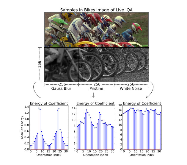 Figure 1
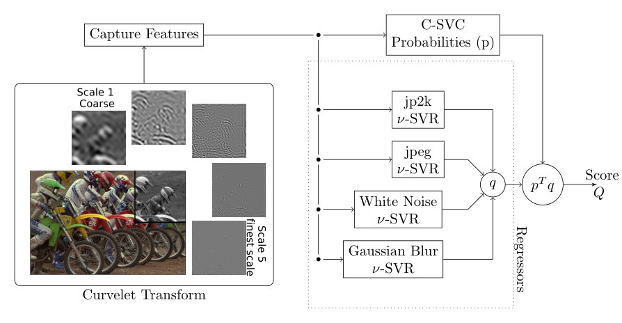 Figure 2
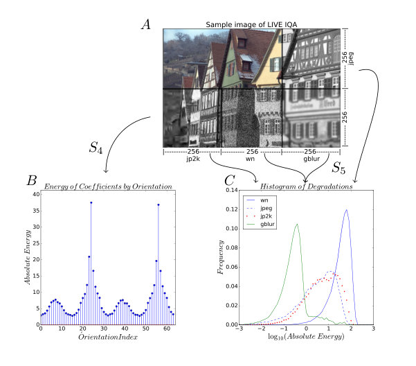 Figure 3
| jp2k | jpeg | wn | gblu | ||
| LIVE IQA 20% | |||||
| SROCC | M1 | 0,8743 | 0,8805 | 1 | 0,9045 |
| Curvelt2014[4] | 0,8373 | 0.9309 | 0,9990 | 0,9175 | |
| KROCC | M1 | 0,7867 | 0,8116 | 1 | 0,8850 |
| Curvelet2014[4] | 0,7337 | 0,8676 | 0,9980 | 0,8830 | |
| TID2013 | |||||
| SROCC | M1 | 0,8447 | 0,8365 | 0,9058 | 0,8548 |
| Curvelt2014[4] | 0.7703 | 0,8337 | 0,8784 | 0,8608 | |
| KROCC | M1 | 0,6467 | 0,6337 | 0.7284 | 0,6592 |
| Curvelet2014[4] | 0,5742 | 0,6353 | 0,6967 | 0,6658 | |
| CSIQ | |||||
| SROCC | M1 | 0,7964 | 0,7747 | 0,8875 | 0,7836 |
| Curvelt2014[4] | 0,7252 | 0,7861 | 0,8674 | 0,7105 | |
| KROCC | M1 | 0,5868 | 0,5670 | 0,6989 | 0,6070 |
| Curvelet2014[4] | 0,5230 | 0,5750 | 0,6773 | 0,5255 | |
Peer Reviews
No public reviews on file for this paper yet. If you reviewed it on a platform where reviews are public (OpenReview, ICLR, NeurIPS, ICML), you can paste yours below so the community can read it here.
Code & Models
Videos
No videos yet. Explain this paper in a talk, walkthrough, or lecture? Add one.
Taxonomy
TopicsImage and Video Quality Assessment · Advanced Image Fusion Techniques · Image and Signal Denoising Methods
Robust statistics and no-reference image quality assessment in Curvelet domain.
Ramon Giostri Campos, Evandro Ottoni Teatini Salles
Programa de Pós-Graduação em Engenharia Elétrica
Universidade Federal do Espírito Santo
Vitória, ES, 29075-910, Brasil
Email:[email protected], [email protected]
Abstract
This paper uses robust statistics and curvelet transform to learn a general-purpose no-reference (NR) image quality assessment (IQA) model. The new approach, here called M1, competes with the Curvelet Quality Assessment proposed in 2014 (Curvelet2014). The central idea is to use descriptors based on robust statistics to extract features and predict the human opinion about degraded images. To show the consistency of the method the model is tested with 3 different datasets, LIVE IQA, TID2013 and CSIQ. To test evaluation, it is used the Wilcoxon test to verify the statistical significance of results and promote an accurate comparison between new model M1 and Curvelet2014. The results show a gain when robust statistics are used as descriptor.
Index Terms:
Image quality assessment (IQA), No reference (NR), Curvelet, Support Vector Machine (SVM), Natural scene images
I Introduction
This is a non-doubly blind version of the article accepted for publication in the XIV Workshop de Visão Computacional111http://www.wvc2018.com.br/proceedings. This version differs from that published only because it has links to download all parts of the software developed and has one additional figure. The software, trained models and some useful routines can be downloaded from the link https://github.com/rgiostri/robustcurvelet.
The Image Quality Assessment (IQA) is an important subject for computational vision, which impacts in robotics, super-resolution, reconstruction of images, evaluation of medical images, among other areas. The research in IQA aim in developing algorithms to make an objective quality score of images (Q) consistent with human opinion, regardless of the content of the image, the level and type of distortion.
This area has three main groups of methods, Full-Reference (FF),Reduced-Reference (RR) and No-Reference (NR). In applied sciences there is usually no reference image, therefore NR methods are appropriate. For research areas like astronomy, microscopy, remote sensing and medical images, the NR models are the unique way to evaluate quality of images without consulting an expert.
This work proposes a NR method, oriented to natural scenes which the features are extracted by the transformed space of curvelets[1]. The traditional Wavelets transform do not have orientation, and orientation facilitates the study of anisotropy in degraded images[2]. The parametrization of Curvelets uses position, scale and orientation, which favors if compared to the traditional Wavelet for this study.
The architecture used in this paper was proposed by Moorthy and Bovik[3] that uses the several modules of Support Vector Machine (SVM) organized in two stages (2-stages SVM).
The complete explanation of 2-stages SVM is in subsection III-D and the flow chart can be viewed in Figure 1.
In the stage 1, the classifier C-support vector classification (C-SVC), provides the probabilities of an image to be of a specific class. In the second stage, each regressor nu-support vector regression (-SVR), provide her prediction. The fusion of predictions is performed by a weighted average. The weights are given by the probability of C-SVC stage.
This work searchs forms to improve the feature extraction in Curvelets space, using robust and non-parametric statistics, which is the main difference for the model proposed by Liu et al.[4], here called Curvelet2014. The two proposals are close by the use of 2-stages SVM, and features extracted in Curvelets space, but are distant by the way the features are extracted.
The propose defined in this paper, called model M1, uses orthodox tools of robust statistics based on quartiles, octiles[5][6] and the Median Absolute Deviation (MAD)[7]. The M1 uses features to describe images and at same time exempts the analysis of outliers and statistical models.
The competing proposes are trained with the LIVE IQA[8] database and tested with the TID2013[9], CSIQ[10] and the LIVE IQA. It is important to mention that because the selected datasets the conclusions are restricted to natural scene images. This type of image is defined as any image obtained on ordinary commercial cameras. The degradation classes used in this paper are compressions jpeg (jpeg) and jpeg2000 (jp2k), Gaussina white noise (wn), Gaussian blur (gblur). One experiment was done using the classes of degradation simultaneously and other experiment for type of degradation. In all the experiments we used the statistical significance test of Wilcoxon[11] to make strengthen conclusions.
All choices made in this article are shown to facilitate their use and reproducibility. An examples of the code can be downloaded in github page https://github.com/rgiostri/robustcurvelet.
The contributions of this article to the scientific community are: 1) Propose a new ways to extract features in the transformed space of Curvelets. These features are based on robust statistical descriptors. 2) Replace the model Curvelet2014, due to the better performance of the new method, which is less dependent on training data and has a better correlation with human perception. The final product is a competitive, open source and reproducible IQA method.
The organization of this work is as follows: In Section II shows a review of the work related to NR IQA, focusing mainly on the use of the Curvelet transform. In Section III shows the invocation. In Section IV presents the methodology. In Section V shows the experiments, results and discussions. Finally, in Section VI the conclusions of the study are shown.
II Related Works
This work uses the second generation Curvelets transform proposed by Candes et al.[1], called Fast Discret Curvelet Transform (FDCT). The implementation used was the Frequency Wrapping (FDCT-Wrap), avaliable for download on the website of CurveLab222http://www.curvelet.org/. The binding with python used was PyCurvelab, available here333https://github.com/slimgroup/PyCurvelab.
The first use of FDCT in NR IQA proposals was made by Shen et al.[12], using only the finest layer for feature extraction.
The architecture 2-stages SVM was introduced by Moorthy and Bovik[3] applied to features extracted from natural scenes. This architecture was used in by [13][14][15][16] with different features.
The use of FDCT with 2-stages SVM was proposed by Liu et al.[4]. Zhao et al.[13] proposed an NR IQA method that uses the entropy of the Curvelet transform coefficients, also associated with the 2-stages SVM. Ahmed e Der[14] used the method proposed in [4] with the spatial features for study of contrast in images. Recently Shahkolaei et al.[17] use the model Curvelet2014[4] to quantify the quality of images associated with historical documents.
Examples of NR IQA work using non-parametric statistics associated with the Curvelet transform can be found in [12][13]. On the other hand, in the literature review, the authors did not find any work in NR IQA that made use of robust statistical tools to extract features from the Curvelets space.
III Proposed Aproach
III-A Pre-processing
Follow [1], the total number of Curvelet coefficients and the total number of scales () depends on the image size (M,N) and the number of directions () on second coarse scale (). This work uses 32 directions on and all images are fragmented in blocks with size (256,256) pixels. The others scales are: is the coarse layer with only one orientation, with 64 orientations, the fine scale that preserve the information of directions with 64 orientations and the finest scale, but has only one direction.
The input image must be 8 bits. Color images or in other scales must be converted.
III-B Features extractions
The model Curvelet2014[4] has 12 features grouped into 3 brands, Mean Energy by Scale (MES), Orientation Energy Distribution in layer (OED4) and Statistics of finest scale () (SFS5). This division of groups is maintained in this article.
Using the principal component analysis (PCA) in 12 original features of Curvelet2014, reveals 3 eigenvalues equal zero, this indicates that 3 out of 12 features are redundant.
III-B1 Mean Energy by Scale (MES)
The authors of [4] proposes the application of on all the coefficients of the transform and the calculation of the mean per scale, as follows:
[TABLE]
where is the mean value of energy scale and is the set of coefficients on scale with orientation .
In [4],the authors make subtractions with energies (1) between the adjacent scales and interval scales. By inspection, it is possible to see that here live 2 of the 3 redundant features.
In other hand, the model M1 uses 3 combinations to discriminate the behavior of the coarser layers, , e . There is no redundancy between these features.
III-B2 Orientation Energy Distribution (OED4)
In mathematics, the anisotropy is the existence of a preferential direction. In images of natural scenes, textures and edges are sources of anisotropy[2].
In [2] it is showed how the addition of white Gaussian noise (wn) and the Gaussian blurring process (gblur) impact on anisotropy measurements of the images. Also in [2] it is said that artifacts created in compression like jpeg and jpeg2000 (jp2k) are difficult to handle.
In [18] the authors argue the degradations affect the high-frequency components of the images. For model M1, the scale is the fine scale with different directions. The is the main source information for the study of anisotropy using the Curvelet transform.
There are more than 98 thousand coefficients in the scale, organized in a matrices and each matrix has 64 orientations (). The average energy per orientation in the layer can be measured as follows,
[TABLE]
where define the mean of coefficients in by direction and direction index has 64 values.
The Figure 2-A shows an image divided in 5 parts. The color part was preserved and the remaining parts were degraded. The Figure 2-B shows the graphics vs for the jp2k part. In this image it is possible see the prominent points in the data. The Figure 3 shows the behavior for classes Gaussian Blur (gblur), Gaussian white noise (wn) and the reference image.
In [19], the authors argue that robust statistics means being callous to small deviations in assumptions. Since one of the sources of deviation is the outliers, then a strategy involving robust statistical descriptors is justified.
Two complementary measures of dispersion are calculated in the scale .
The first estimator is Quartile coefficient of dispersion (QCD)[20],
[TABLE]
.
where and are first and third quartiles of data (2).
The second estimator is MAD[7] divided by median,
[TABLE]
where computes the median, is the median of the data (2).
The third feature in is the area below the curve of the data (2).
All model-free features, applied to data directly.
III-B3 Statistics of finest scale (SFS5)
For Shen et al.[12], propose the transformation of the coefficients grouped into ,
[TABLE]
where is the set of coefficients in scale 5.
In Figure 2-C shows the histogram of the probability distribution by type of degradation, what exposes several formats of distributions.
Several formats of distribution imply studying asymmetry and flattening of distributions. The lack of the normality condition and the presence of outliers justify doing this research with robust statistical descriptors[19].
The robust descriptors in SFS5 are better understood using the octiles concept, which divides the sample into 8 sections of equal size, to . This method is applied directly to the coefficients transformed by (5) without requiring a histogram or curve fit.
The first three descriptors are the median , interquartile range () and the MAD estimator .
The fourth descriptor is the Bowley Skewness[5],
[TABLE]
the fifth feature is Moors Kurtosis[6],
[TABLE]
where the octiles are define with percentiles, , , , , , , , besides for .
III-C Post Processing
Remembering, the model M1 has 11 features without redundancy, 3 in MES, 3 in OED4 and 5 in SFS5, calculated for each gray scale block.
For each input image, the number of blocks varies according its size. The 11 features are calculate for each block. The simple mean of each features make the 11-dimension vector. This vector represent the input image on features space and is the input of 2-stages SVM for machine learnig.
III-D Architecture 2-stages SVM
In this work, the 2-stages SVM uses the 11-dimension vector obtained by the coefficients of the Curvelet transform. This vector passes through ensemble of regressors. The predictions of regressors are fused using mean weight. The weights are provided by the classifier.
In Figure 1, 4 branches in dashed box show the set of regressors. Each regressor uses an -SVR with Radial Base Funcition (RBF) kernel. Each regressor was trained with degraded images of a specific class, becoming a specialist in that class.
For this work, the set of regressors returns a column vector with the predictions of each regressor.
Also in Figure 1, the upper branch is the classifier. We used a C-SVC with output in probability and an RBF kernel. The output of classificator is a column vector .
Each module can be approached independently. In this work, the only additional procedure was the application of a standardized scale transformation (zero mean and unit variance) for each block.
When a test image is inserted in this architecture, it passes through the classifier and the 4 regressors. The objective quality index is the weighted average of the predictions of the regressors bank, expressed by,
[TABLE]
IV Methodology
IV-A Data set of images
IV-A1 LIVE IQA
The set LIVE IQA[8]444http://live.ece.utexas.edu/research/quality/subjective.htm has 29 reference images of natural scenes. From them they create 779 degraded images, distribute in 5 categories. The subjective quality index used in the LIVE IQA survey is the Differential Mean Opinion Scores (DMOS) with values between 0 and 100, where 0 values indicates the highest quality.
In this work we will use only 4 classes: jpeg (jpeg) compression and jpeg2000 (jp2k), white noise Gaussian (wn), Gaussian blur (gblur), total number of 634 degraded images.
IV-A2 TID2013
The set TID2013[9]555http://www.ponomarenko.info/tid2013/tid2013.rar has 25 reference images, 24 of natural scenes and one artificial. It has 25 classes of distortion with 5 levels of degradation per class, having a total of 3125 degraded images with standard size . The subjective quality index is the Mean Opinion Scores (DMOS) with values between 0 and 9, where 9 values indicates the highest quality.
For the experiments of this work only the natural images and the 4 classes used in LIVE IQA . The total of the images used is 480.
IV-A3 CSIQ
The set CSIQ[10]666http://vision.eng.shizuoka.ac.jp/mod/page/view.php?id=23 has 30 reference images. There are 6 classes of distortion and 5 levels of degradation per class, generating a total of 900 degraded images of standard size . The subjective quality index used in the CSIQ survey is the Differential Mean Opinion Scores (DMOS) with values between 0 and 1, where 0 values indicates the highest quality.
In the experiments, four previously mentioned categories were used. The total of 600 degraded images.
The data set LIVE IQA and TID2013 has the same primary font for reference images, a set of public images Kodak Lossless True Color Image Suite777http://r0k.us/graphics/kodak/[9]. To perform an experiment absolutely independent of any bias resulting from this content overlap we use the CSIQ data set.
IV-B Machine Learning
The following steps are applied to model M1 and concurrent job Curvelet2014 [4].
In this work, the training is performed with the degraded images of LIVE IQA.
By [3] and [4], the training set should be separated using the reference images. This prevents content overlap in the test involving LIVE IQA.
The separation of degraded images is done by mapping reference images. We use 5-fold method with 40 repetitions to cover a large number of possibilities of association of reference images. This makes a 200 different sets to train. The training is done with the degraded images mapped using 80% of the reference images in each set. The rest of the degraded images, are used in the test phasis.
After training, the models are tested separately using 20 % of the degraded images of the LIVE IQA, 480 images of the TID2013 set and 600 images of the CSIQ set.
The SVM hyperparameters must be obtained for each training set[3].
For each round the hyperparameters are computed for C-SVC using the stratified 5-fold cross-validation method with 5 random repetitions. As same, it is computed to each regressor -SVR the hyperparameters using 5-fold cross-validation method with 5 random repetitions. The search grids for each of the hyperparameters were , . The parameter was set at 0.5 because tests using a search grid between 0.25 and 0.75 showed minimal variation of results.
This computational implementation was performed using the python scikit-learn 0.19.1 package888https://scikit-learn.org/stable/.
IV-C Quality Measures of Predictions
The main product of NR methods is the objective quality index(Q). The quality of the prediction is measured using correlation between Q index of the images and the subjective index associated of the images (DMOS or MOS).
Ponomarenko et al.[9] recommend the Spearman’s rho (SROCC) and the Kendall’s tau (KROCC) as correlation measures. Values close to 1 indicate a better correlation with human perception.
To measure the quality of the classifier the accuracy is used. Values closer to 1 indicate a better classification.
IV-C1 Statistical significance
Statistical significance: Due to the structural proximity between the competing models, we chose a statistical significance test to support more accurate conclusions. And, when normality and homoscedasticity tests indicate that there is no distribution common to all experiments non-parametric test is recommended.
The way the experiments were conducted generates paired results. The Paired Samples Wilcoxon Test[11] is adequate and was used in the measures of SROCC, KROCC and accuracy of the M1 and Curvelet2014.
For this test the null hypothesis is: The means of the groups compared is identical. The alternative hypothesis is: The means are different.
In this article the null hypothesis is rejected for value , the comparisons in which this occurs the mean of greater value is highlighted. There is greater interest in cases where the null hypothesis is rejected. It is known that the rejection of the null hypothesis does not imply accepting the alternative hypothesis.
The Wilcoxon test will only allow a simple and reasonable conjecture that there is evidence to believe that the highest average model has a better result.
To strengthen this conjecture, we will emphasize results that are persistent in at least 2 tests and that there is no setback in the remaining tests.
This computational implementation is performed in subsection IV-C were made using the scipy 1.1.0 python package999https://www.scipy.org/.
V Experiments and Results
We made two types of experiments. The first evaluating the overall result using the four classes of degradation simultaneously and the second evaluating the result by class.
The cells of Tables I and II should be evaluated in pairs (white and gray). There is more emphasis in the analysis by columns, they go through the 3 tests. Do not compare the values of SROCC and KROCC because they evaluate different forms of correlation.
V-A Four Classes test
This experiment consists of testing competing models with all test images. The outputs and the output of the classifier are collected. Predictions are compared to subjective quality index and degraded image label.
The same sets of images are used for training and testing in both models over 200 rounds.
The analysis of Table I column by column shows that the M1 classify demonstrates better than Curvelet2014.
Also in Table I SROCC indicates that in 2 tests the null hypothesis is verified. On the other hand KROCC presents 2 results in which it is rejected, both favorable to the model M1.
Separating table I by test, M1 shows better results in the LIVE IQA 20% and CSIQ tests. The test performed with TID2013 shows statistically equivalent results.
In this experiment there were 6 favorable results for M1, 3 indifferent results for the M1 model and none was unfavorable.
V-B Performance by class of degradation
This experiment discriminates which degradations are best described by each model. To do this, the prediction is made using only images of a particular degradation class, and the accuracy is not evaluated.
Four different experiments are performed, one for each class of degradation. The results are grouped in the Table II.
The analysis of Table II column by column shows that M1 has superior performance in the jp2k and wn classes. For jpeg class KROCC gave indications that Curvelet2014 is better to describes this class, but this conclusion is contradicted by the SROCC test of TID2013. The gblur class does not present results that are favorable to any model.
There was no systematic behavior for the averages of the gblur class. It is possible to make a variation analysis, where smaller variations are preferable to larger ones.
In this analysis for class gblur, it is verified that M1 is superior to the competitor. The model M1 has variations 12.1% for SROCC and 27.8% for KROCC. The model Curvelet2014 has variatons 20.6% for SROCC and 35.7% for KROCC.
In this experiment there were 13 favorable results for M1, 2 indifferent results for the M1 model and 6 unfavorable results.
VI Conclusion
In this work, an objective method was developed to evaluate image quality without reference image, acronym (NR IQA). The method consists in extracting 11 features within the transformed space of the Curvelets and has as a differential the use of robust statistical descriptors. The proposed model M1 positions itself as an alternative to the model proposed in [4], Curvelet2014. The models were tested with 3 databases of natural scenes images.
The M1 model classify better than Curvelet2014 according to Table I. The probable hypothesis is that the features of M1 are more discriminatory for classification, there were already indications of this in the transformation of principal components for the 12 characteristics of Curvelet2014.
Also, Table I shows improvements in agreement between Q and subjective indexes (DMOS and MOS) in a multi-class experiment. In such experiment, 6 of them give favorable results for M1, 3 of them give indifferent results for the M1 model and none was unfavorable.
The M1 model also presents the highest correlation for the jp2k class for all tests and correlations. The most likely hypothesis is that robust statistical descriptors will better discriminate the data from the jp2k class. This class is quite problematic, as shown in Figure 2 this class can present outliers in and has a no normal distribution of coefficients in .
The class jpeg presents a KROCC measure in favor of the model Curvelet2014. This indication is not strong, because is contradicted by a SROCC test.
The M1 model presents a better correlation for the degradation of the white Gaussian noise type (wn) in most tests. There was no evidence of the contrary.
For Gaussian blurring degradation (gblur) the M1 model presented more robust and unbias results. It is callous to bias introduced by training in a specific database. This last statement is also endorsed by superior performance in the CSIQ database.
The statistical tests performed showed that, more often, M1 model presented superior results. M1 presented higher correlation with statistically significant in almost all the tests and with smaller numerical variation among the databases.
For these reasons the M1 model is the most advantageous option among the models tested.
The reference list from the paper itself. Each links out to its DOI / PubMed record.
- 1[1] E. D. L. Candès, D. Donoho, and L. Ying, “Fast Discrete Curvelet Transforms,” Multiscale Modeling and Simulation , vol. 5, no. 3, 2006.
- 2[2] S. Gabarda and G. Cristóbal, “Blind image quality assessment through anisotropy,” J. Opt. Soc. Am. A , vol. 24, no. 12, pp. B 42—-B 51, 2007.
- 3[3] A. K. Moorthy and A. C. Bovik, “A Two-Step Framework for Constructing Blind Image Quality Indices,” IEEE Signal Processing Letters , vol. 17, no. 5, pp. 513–516, 2010.
- 4[4] D. Liu Lixiong, H. H. Hongping, and B. A. C, “No-reference image quality assessment in curvelet domain,” Signal Processing: Image Communication , vol. 29, no. 4, 2014.
- 5[5] R. A. Groeneveld and G. Meeden, “Measuring skewness and kurtosis,” Journal of the Royal Statistical Society. Series D (The Statistician) , vol. 33, no. 4, pp. 391–399, 1984.
- 6[6] J. J. A. Moors, “A quantile alternative for kurtosis,” Journal of the Royal Statistical Society. Series D (The Statistician) , vol. 37, no. 1, pp. 25–32, 1988.
- 7[7] P. J. Rousseeuw and C. Croux, “Alternatives to the median absolute deviation,” Journal of the American Statistical Association , vol. 88, no. 424, pp. 1273–1283, 1993.
- 8[8] H. R. Sheikh, Z. Wang, L. Cormack, and A. C. Bovik, “Live image quality assessment database release 2.” [Online]. Available: http://live.ece.utexas.edu/research/quality/