On the Rotational Invariant $L_1$-Norm PCA
Sebastian Neumayer, Max Nimmer, Simon Setzer, Gabriele Steidl

TL;DR
This paper reinterprets the rotational invariant $L_1$-norm PCA as a gradient-based optimization on Grassmannian manifolds, proving convergence to critical points using the Kurdyka-Łojasiewicz property.
Contribution
It provides a novel interpretation of robust $L_1$-norm PCA as a gradient descent on Grassmannian manifolds and establishes convergence results for the entire iterative process.
Findings
Reinterpreted $L_1$-norm PCA as a gradient descent on Grassmannian manifolds.
Proved convergence of all iterates to a critical point using Kurdyka-Łojasiewicz property.
Unified robust PCA methods under a geometric optimization framework.
Abstract
Principal component analysis (PCA) is a powerful tool for dimensionality reduction. Unfortunately, it is sensitive to outliers, so that various robust PCA variants were proposed in the literature. Among them the so-called rotational invariant -norm PCA is rather popular. In this paper, we reinterpret this robust method as conditional gradient algorithm and show moreover that it coincides with a gradient descent algorithm on Grassmannian manifolds. Based on this point of view, we prove for the first time convergence of the whole series of iterates to a critical point using the Kurdyka-{\L}ojasiewicz property of the energy functional.
Click any figure to enlarge with its caption.
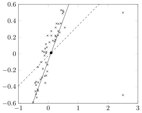 Figure 1
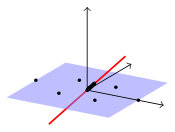 Figure 2
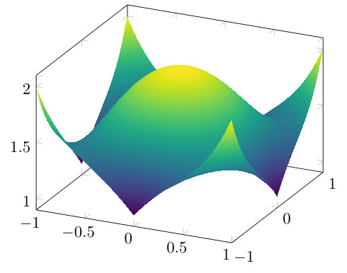 Figure 3
Peer Reviews
No public reviews on file for this paper yet. If you reviewed it on a platform where reviews are public (OpenReview, ICLR, NeurIPS, ICML), you can paste yours below so the community can read it here.
Videos
No videos yet. Explain this paper in a talk, walkthrough, or lecture? Add one.
\setkomafont
sectioning \setkomafonttitle \setkomafontdescriptionlabel
On the Rotational Invariant -Norm PCA
Sebastian Neumayer111Department of Mathematics, Technische Universität Kaiserslautern, Paul-Ehrlich-Str. 31, D-67663 Kaiserslautern, Germany, {neumayer,nimmer,steidl}@mathematik.uni-kl.de.
Max Nimmer111Department of Mathematics, Technische Universität Kaiserslautern, Paul-Ehrlich-Str. 31, D-67663 Kaiserslautern, Germany, {neumayer,nimmer,steidl}@mathematik.uni-kl.de. 444corresponding author
Simon Setzer333Engineers Gate, London, United Kingdom
Gabriele Steidl111Department of Mathematics, Technische Universität Kaiserslautern, Paul-Ehrlich-Str. 31, D-67663 Kaiserslautern, Germany, {neumayer,nimmer,steidl}@mathematik.uni-kl.de. 222Fraunhofer ITWM, Fraunhofer-Platz 1, D-67663 Kaiserslautern, Germany
Abstract
Principal component analysis (PCA) is a powerful tool for dimensionality reduction. Unfortunately, it is sensitive to outliers, so that various robust PCA variants were proposed in the literature. One of the most frequently applied methods for high dimensional data reduction is the rotational invariant -norm PCA of Ding and coworkers. So far no convergence proof for this algorithm was available. The main topic of this paper is to fill this gap. We reinterpret this robust approach as a conditional gradient algorithm and show moreover that it coincides with a gradient descent algorithm on Grassmannian manifolds. Based on the latter point of view, we prove global convergence of the whole series of iterates to a critical point using the Kurdyka-Łojasiewicz property of the objective function, where we have to pay special attention to so-called anchor points, where the function is not differentiable.
Keywords: Principal component analysis, Dimensionality reduction, Robust subspace fitting, Conditional gradient algorithm, Frank-Wolfe algorithm, Optimization on Grassmannian manifolds
MSC: 58C05, 62H25, 65K10
1 Introduction
In exploratory data analysis, principal component analysis (PCA) [37] still is one of the most popular tools for dimensionality reduction. Given data points , it finds a -dimensional affine subspace , , of having smallest squared Euclidean distance from the data:
[TABLE]
where denotes the Euclidean norm. While in the above minimization problem is not unique, every minimizing affine subspace goes through the offset(bias) . Therefore, we restrict our attention to data points , , and subspaces through the origin minimizing the squared Euclidean distances to the , . Setting further the gradient with respect to to zero and allowing only orthonormal columns in , the PCA problem becomes
[TABLE]
where
[TABLE]
denotes the orthogonal projection onto and the identity matrix. Here denotes the range and the kernel of . One convenient property of PCA is the nestedness of the PCA subspaces, i.e., for , the optimal -dimensional PCA subspace is contained in the -dimensional one. Furthermore, it is very fast, as the columns of an optimal are the eigenvectors corresponding to the largest eigenvalues of the empirical covariance matrix which can be computed in polynomial time.
Unfortunately, PCA is sensitive to outliers appearing quite often in real-world data sets, see Fig. 1. A lot of different methods in robust statistics [14, 24, 29] and optimization were proposed to make the dimensionality reduction more robust. One possibility consists of removing outliers before computing the principal components which has the serious drawback that outliers are difficult to identify and other data points are often falsely labeled as outliers. Another approach assigns different weights to data points based on their estimated relevancy, to get a weighted PCA, see, e.g. [18]. The RANSAC algorithm [10] repeatedly estimates the model parameters from a random subset of the data points until a satisfactory result is obtained as indicated by the number of data points within a certain error threshold. In a similar vein, least trimmed squares PCA models [38, 40] aim to exclude outliers from the squared error function, but in a deterministic way. The variational model in [6] decomposes the data matrix into a low rank and a sparse part. Related approaches such as [31, 43] separate the low rank component from the column sparse one using different norms in the variational model. However, such a decomposition is not always realistic. From a statistical point of view, robust subspace recovery can be done via Tyler’s M-estimator [41, 44], a special case of M-estimators of covariance. But due to the large number of variables to be estimated for the scatter matrix, this approach is not feasible for high dimensional data. Another group of robust PCA approaches replaces the squared norm in the PCA by the norm. Then, the minimization of the energy functional can be addressed by linear programming, see, e.g., Ke and Kanade [16]. Unfortunately, this norm is not rotationally invariant meaning that in general for an orthogonal matrix we have . Consequently, when rotating the centered data points , the minimizing subspace is not rotated in the same way.
In this paper, the focus lies on the model
[TABLE]
where in contrast to (1) we do not square the Euclidean norm. First of all, let us mention that the determination of the offset is not straightforward now. Frequently, the geometric median of the data is used as offset, which is in general not a minimizer of (3), see [33, Sect. 5]. However, in this paper it is assumed that is fixed and already subtracted from the data. Then, (3) reduces to
[TABLE]
A slightly different form of this model became popular under the name rotational invariant -norm PCA by a paper of Ding et al. [8].
It is important to note that in contrast to the classical PCA the hierarchical structure of the approach is lost. This is exemplified in Fig. 2. We mention that several models applying the deflation technique of standard PCA in a robust setting were also provided in the literature. These models are not of interest in this paper, but we refer to the book [13, p. 203] and the collection of papers [12, 17, 20, 23, 25, 31, 35] which is clearly not complete.
Despite the loss of the nestedness property and the non-smooth target function which is harder to optimize, the robustness makes (4) an attractive choice in practical problems. Examples of improved performance compared to standard PCA and other robust alternatives can be found in, e.g., [8, 22]. Furthermore, in [30] it was shown that under certain assumptions on the given so-called inlier and outlier data, by minimizing (4) we can recover the exact underlying subspace spanned by the inlier data points. Additionally, in contrast to convex relaxation methods, the approach is well suited for high dimensional data appearing, e.g., in image processing.
The minimization of (4) has been treated before. Ding et al. [8] suggest a constrained minimization based on a power method without convergence proof. In [30] the optimization problem is tackled by a geodesic gradient descent approach on the Grassmannian and under certain assumptions on the data, local convergence to the global minimizer is shown for an appropriate starting step size and initial iterate. A tight convex relaxation was studied in [23], where the projection matrix is estimated. Due to the much larger size of the projection matrix, this approach is not suitable for high-dimensional data. An approach based on iteratively reweighted least squares can be found in [21], where standard PCA is repeatedly applied to rescaled data points. For the special case of one-dimensional subspaces (), a Weiszfeld-like algorithm with convergence was given in [33].
In this paper, the iterative algorithm of Ding et al. [8] is first interpreted as a conditional gradient algorithm, also known as Frank-Wolfe algorithm, which only implies a certain convergence behavior of subsequences of the iterates. Recalling that we are not interested in the columns of the minimizer in (4) itself, but just in the -dimensional subspace spanned by them, we show that the algorithm can be recast as a gradient descent algorithm on the Grassmannian manifold. This enables us to prove global convergence of the whole sequence of iterates under mild assumptions.
The paper is organized as follows: In Section 2, we recall preliminaries on Stiefel and Grassmannian manifolds. We discuss important properties of the robust PCA functional in Section 3. Section 4 shows the equivalence of the algorithm of Ding et al. [8], the conditional gradient algorithm and a gradient descent algorithm on Grassmannians. The proof of global convergence of the whole sequence of iterates under some restrictions on the so-called anchor points is given in Section 5. Finally, Section 6 addresses the topic of anchor points.
2 Preliminaries on Stiefel and Grassmannian Manifolds
In this section, we briefly provide the basic notation on Stiefel and Grassmannian manifolds which is required in our approach. Good references on the topic, in particular for optimization on these manifolds, are [1, 9].
Let . The (compact) Stiefel manifold is defined by
[TABLE]
For , it coincides with the unit sphere in and for with the orthogonal matrices . The tangent space at is given by
[TABLE]
where denotes a matrix with orthonormal columns which are in addition orthogonal to the columns of . There are two common ways to define inner products on the tangent space such that becomes a Riemannian manifold, namely
- i)
the Frobenius inner product , or
- ii)
the canonical inner product \langle H_{1},H_{2}\rangle_{A}\coloneqq\operatorname{tr}\bigl{(}H_{1}^{\mathrm{T}}(I_{d}-\frac{1}{2}AA^{\mathrm{T}})H_{2}\bigr{)}.
In the rest of this paper always denotes the Frobenius norm of . The first inner product appears when considering as submanifold of the Euclidean space , while the second one relies the quotient structure . We are mainly interested in the -dimensional subspace spanned by the columns of , which does not change if we multiply from the right with an orthogonal matrix . This is pictured by the Grassmannian manifold, or just Grassmannian, which can be defined as quotient manifold of the Stiefel manifold . The equivalence classes belonging to can be represented by elements of the Stiefel manifold. The tangent space of at can be identified with its horizontal lift at ,
[TABLE]
Further, the Grassmannian becomes a Riemannian manifold by reducing the Riemannian metrics in i) or equivalently ii) to , i.e., for any representative and ,
[TABLE]
A possible choice for a metric on the Grassmannian is given by
[TABLE]
where and is the spectral norm.
In PCA we aim to find an optimal subspace, which means that we are interested in elements of Grassmannians. In practice, working with equivalence classes is difficult and hence calculations are performed with representatives on the Stiefel manifold.
The proposed optimization algorithms involve the orthogonal projection , i.e.,
[TABLE]
To this end, recall that the polar decomposition of a matrix is given by , where and is symmetric and positive semi-definite. Starting with the (economy-size) singular value decomposition , where , is a diagonal matrix and and , the polar decomposition is determined by and . The following lemma can be found e.g. in [15, 38].
Lemma 2.1**.**
The orthogonal projection is given by
[TABLE]
If has full rank, then .
3 Model Analysis
The main focus of this section lies on investigating the objective function in (4) and a related function with respect to differentiability and convexity. To be precise, we are actually only interested in minimizing over equivalence classes . Besides the objective function
[TABLE]
we also deal with the function
[TABLE]
Clearly, these two functions take the same values on the Stiefel manifold . However, they have quite different properties as functions on , but this was often neglected in existing approaches. While is well-defined on the whole , the function is only well defined on the closed domain
[TABLE]
and therefore it is extended to the whole by
[TABLE]
For and all , it holds so that . Further, if and only if for some . The compact subset of
[TABLE]
is called anchor set.
In the simple case and , the above functions read and with . While the first function is locally Lipschitz continuous on , the second one does not have this property at . The following two lemmata state properties of and .
Lemma 3.1**.**
The function defined by (7) is locally Lipschitz continuous on .
Proof.
It suffices to show the property for the summands . For an arbitrary fixed , let , . Then, we obtain
[TABLE]
∎
In general, the function is neither convex nor concave on , see Fig. 3.
In contrast, is concave as the following lemma shows.
Lemma 3.2**.**
The function defined by (8) and (10) fulfills the following relations:
* is convex.* 2. 2.
* is convex.* 3. 3.
The subdifferential of is empty at the boundary of , i.e. at with for some .
Proof.
It holds if and only if
[TABLE]
for all . Since the intersection of convex sets is convex, it suffices to show convexity of separately. Let . Then, using (12), we obtain for that
[TABLE]
Thus, and the claim follows. 2. 2.
Since the sum of concave functions is concave again, it suffices to consider the individual summands again. For , we define
[TABLE]
which is differentiable on an open set containing . By the chain rule and since , the gradient of is
[TABLE]
Using the product rule and the chain rule, the Hessian is given by
[TABLE]
for all so that
[TABLE]
Consequently, the Hessian is negative semidefinite and concave in for all . Finally,
[TABLE]
is concave as the pointwise infimum of a family of concave functions. 3. 3.
For an arbitrary fixed , let with . We consider the subdifferential of at given by
[TABLE]
Choosing with , a subgradient must fulfill
[TABLE]
which leads to a contradiction if . Hence, the subdifferential is empty.
∎
For the algorithms the gradient and the Riemannian gradient on the Grassmannian of the functions and are required.
Lemma 3.3**.**
Let and be defined by (7) and (8), respectively. Then, the gradient and the Riemannian gradient on at are given by
[TABLE]
where
[TABLE]
Note that is also the horizontal lift of the gradient on the Grassmannian at , where and is the projection from onto .
Proof.
By straightforward computation we obtain for that
[TABLE]
For the gradient of coincides with the Riemannian gradient of on , i.e.,
[TABLE]
This implies the assertion. ∎
We call a critical point of , resp. if
[TABLE]
4 Minimization Algorithm
In this section, we show that the constrained minimization algorithm of Ding et al. [8] can be interpreted as i) a conditional gradient algorithm, and ii) a gradient descent algorithm on Grassmannians. The conditional gradient algorithm, also known as Frank-Wolfe algorithm, was originally proposed 1956 in [11] for solving linearly constrained quadratic programs and was later adapted to other problems. For a good overview, we refer to [27] and the references therein. Then it follows from general results on the algorithm that a subsequence of the iterates converges under strong conditions on the anchor points to a critical point of the functional.
Constrained Minimization Algorithm.
Ding et al. [8] consider the constrained optimization problem
[TABLE]
The authors claimed without proof that the function is convex in and has a unique global minimizer. Both statements are not correct: for and it is easy to check that is concave in ; for , , with centered data points and the minimizers of are given by and , which span different subspaces. Penalizing the constraint in (16) via a symmetric Lagrange multiplier , setting the gradient of the resulting Lagrangian with respect to to zero and applying an orthogonalization procedure, see Lemma 2.1, the authors arrive at the following iteration scheme: if ,
[TABLE]
Conditional Gradient Algorithm.
The conditional gradient algorithm is commonly used to minimize a convex function over a compact set. However, as in [27], we apply it for maximizing the convex function .
In general, for a proper convex function and a nonempty, compact set , the conditional gradient algorithm is the update scheme
[TABLE]
Note that according to [39, Corollary 32.4.1], the value is a local maximizer of over if for all ,
[TABLE]
By definition of the subdifferential we have
[TABLE]
where the last equation follows by choosing .
For finite convex functions the following convergence result was proved in [27] based on [28]. The proof can be modified for with values in the extended real numbers and in a straightforward way.
Theorem 4.1**.**
Let a proper convex function and a nonempty, compact set. Then the sequence generated by (18) is strictly increasing except when , in which case it terminates at satisfying (19). If is continuously differentiable on , then every accumulation point of the sequence fulfills (19).
We want to apply the scheme (18) for and , where
[TABLE]
denotes the set of matrices in having a distance smaller than some from the anchor set. To this end, the maximization problem (18) has to be solved, but first we have to find a suitable . For this purpose define the iteration
[TABLE]
for , where we plugged as given in Lemma 3.3 into (18). Now, assume that we can find such that for all . In this case
[TABLE]
Note that we can always find such an for large enough if all accumulation points of as in (21) are non-anchor points. Using Lemma 2.1 we obtain
[TABLE]
which is exactly the iteration scheme (17) proposed by Ding et al. Based on Theorem 4.1, we have the following corollary for our special setting.
Corollary 4.2**.**
Let be defined by (8)-(10). Assume that the sequence generated by (22) has no element in and that the set of accumulation points has a positive distance from . Then the sequence is strictly decreasing except for iterates where
[TABLE]
in which case the iteration terminates at which is a critical point. Condition (23) is equivalent to , resp. to . If the iteration does not terminate after a finite number of steps, every accumulation point of is a critical point.
Proof.
We show that the three stopping criteria are equivalent. Let and recall that .
-
If , then and thus .
-
If , then and thus
[TABLE]
Further, this implies (23).
- Assume now that (23) is fulfilled. Then, we have
[TABLE]
On the other hand, we have with that
[TABLE]
where denotes the largest eigenvalue of the matrix . Hence, .
It remains to show that all accumulation points of infinite sequences are critical points. Let be an accumulation point of such a sequence. As the set of accumulation points has positive distance from , we can choose small enough such that all iterates are in for large enough. Then, by Theorem 4.1, the accumulation point fulfills (19) and as is differentiable in , this implies that is a critical point. ∎
Remark 4.3**.**
Unfortunately, the function has no subdifferential at the boundary of its domain and touches this boundary in the anchor set. A remedy would be to use instead of the function
[TABLE]
By the proof of Lemma 3.2, we conclude that is convex on an open set which contains and therefore also . Thus, accumulation points of the sequence produced by the conditional gradient algorithm are critical points by Theorem 4.1. Another idea consists of switching to a function with summands , where is e.g. the Huber function as proposed in [8]. This approach is not pursued any further, since we are more interested in finding an algorithm for the original function without an additional parameter.
Gradient Descent Algorithm on .
By (15), a matrix is a critical point of , resp. , on if and only if . This can be rewritten as
[TABLE]
where is assumed to be invertible which is the case under the reasonable assumption that and , where .
Remark 4.4**.**
Note that . Let be an eigenvalue decomposition with eigenvalues of in the diagonal matrix . Plugging this into (29), multiplying with from the right and substituting we get
[TABLE]
*so that the columns of are eigenvectors of with eigenvalues .
Using the same relations in (31), we arrive at*
[TABLE]
which allows the interpretation of , as columns-wise step sizes in the gradient descent iteration (32).
Together with Lemma 2.1, the fixed point equation (31) gives rise to the following descent scheme on , resp. :
[TABLE]
Note the strong connection of this iterative scheme to the Weiszfeld algorithm [4, 42, 34] and majorize-minimize strategies [7].
By the following lemma, the gradient descent iteration (32) coincides with those of the conditional gradient algorithm (22) on the Grassmannian .
Lemma 4.5**.**
For the same input matrix , the iterates generated by the schemes (32) and (22) coincide on , i.e., they span the same subspace.
Proof.
Since for , we observe that the matrices produced by the update schemes (32) and (22) span the same subspace as they differ only by a multiplication with an invertible matrix from the right. Since both iterates are in the Stiefel manifold, they can only differ by orthogonal matrix, i.e., for some . ∎
The following lemma quantizes the relation from Corollary 4.2 that is decreasing.
Lemma 4.6**.**
If , then generated by (32) satisfies
[TABLE]
Proof.
In order to shorten notation, we denote and . For it holds so that
[TABLE]
Using , this can be rewritten as
[TABLE]
The first sum can be simplified to
[TABLE]
so that
[TABLE]
∎
5 Convergence Analysis
So far Corollary 4.2 only ensures convergence of a subsequence of the iterates to a critical point under a restrictive assumption on the anchor directions. In this section, we prove global convergence of the whole sequence of iterates generated by algorithm (32) on the Stiefel manifold (and thereby on the Grassmannian) under mild assumptions which are summarized at the end of this section.
The important observation is that both and are semi-algebraic functions. Such functions are typical examples of so-called Kurdyka-Łojasiewicz (KL) functions [2, 19, 26]. A function with Fréchet limiting subdifferential , see [32], is said to have the Kurdyka–Łojasiewicz (KL) property at if there exist , a neighborhood of and a continuous concave function such that
, 2. 2.
is on , 3. 3.
for all it holds , 4. 4.
for all , the Kurdyka–Łojasiewicz inequality holds true.
A proper, lower semi-continuous (lsc) function which satisfies the KL property at each point of is called KL-function. For KL-functions, the following theorem [3, Theorem 2.9] holds true.
Theorem 5.1**.**
Let be a KL function. Let be a sequence which fulfills the following conditions:
- C1)
There exists such that for every . 2. C2)
There exists such that for every there exists with , where denotes the Fréchet limiting subdifferential of **[32]**. 3. C3)
There exists a convergent subsequence with limit and .
Then the whole sequence converges to and is a critical point of in the sense that . Moreover the sequence has finite length, i.e.,
[TABLE]
Similar arguments as used in the proof of Theorem 5.1 lead to the next corollary, see [3, Corollary 2.7].
Corollary 5.2**.**
Let be a KL function. Denote by , and the objects appearing in the definition of the KL function. Let be such that with . Consider a finite sequence , , which satisfies the Conditions C1 and C2 of Theorem 5.1 and additionally
- C4)
, 2. C5)
.
If for all it holds
[TABLE]
then for all .
We start our convergence analysis by showing property C1).
Lemma 5.3**.**
Assume that for all generated by (32). Then, there exists such that
[TABLE]
Proof.
In order to shorten notation, we denote and . By Lemma 4.6 and since , we estimate
[TABLE]
Next, we want to estimate the sum on the right hand side. To this end, note that
[TABLE]
with some unit vector as . The latter follows directly from the fact that the columns of are in . We can choose a basis of from the data points and w.l.o.g., , where . Then, setting , the coefficients can be estimated by for . Setting for all , we obtain
[TABLE]
Using the equivalence of Frobenius and spectral norm, (38) now results in the estimate
[TABLE]
It remains to show that . Since , we get
[TABLE]
where
[TABLE]
All eigenvalues of are in . On the other hand, since , it holds
[TABLE]
Finally, this implies with the smallest eigenvalue of the matrix that
[TABLE]
∎
Corollary 5.4**.**
Assume that for all generated by (32). Then, it holds
[TABLE]
The set of accumulation points of is compact and connected in . Every accumulation point which is not an anchor point is a critical point of , i.e. . The same statements hold true for the corresponding equivalence classes in .
Proof.
- Since is decreasing and bounded below by zero, we know that for some . Multiplying (37) by , summing and taking the limit yields
[TABLE]
Consequently, the series on the right-hand side converges and . Using the estimate
[TABLE]
the statement also holds on .
2. By the theorem of Ostrowski [36, p. 173], it follows that the set of accumulation points of is compact and connected both in and .
3. Since the sequence is bounded, it has a convergent subsequence. Let be a subsequence converging to a non-anchor point and be the update operator in (32), i.e.,
[TABLE]
Then is continuous for which we can see as follows: The projection is continuous on all full rank matrices. For ,
[TABLE]
has only eigenvalues larger than , so that the argument of the projection has full rank. Furthermore, (and therefore ) depends continuously on except for .
Using the continuity of outside , we have . By continuity of , this implies
[TABLE]
By Corollary 4.2, is strictly decreasing except for in which case . ∎
Lemma 5.5**.**
Assume that the elements of the sequence are generated by (32) and the accumulation points do not belong to the anchor set . Then the sequence fulfills C2) in Theorem 5.1, i.e., there exists such that
[TABLE]
Proof.
By the assumptions and Corollary 5.4 the set of accumulation points has a positive distance from . Since , we have for large enough that all lines connecting and are in a compact set for some . Here denotes the ball centered at [math] with radius with respect to the Frobenius norm. Further, is smooth on an open set containing so that the mean value theorem implies
[TABLE]
Hence, we can estimate
[TABLE]
Now, (39) implies
[TABLE]
For the second term, we can use the series expansion of the square root given by
[TABLE]
Plugging this in yields
[TABLE]
From Corollary 5.4 we know that at each accumulation point which is not an anchor point the gradient of is zero, so that . Furthermore, both \lambda_{\mathrm{min}}\bigl{(}S_{A^{(r)}}^{-1}\bigr{)} and \lambda_{\mathrm{max}}\bigl{(}S_{A^{(r)}}^{-1}\bigr{)} depend continuously on on the compact set , so that they can be bounded by their positive minima and maxima on , respectively. Consequently, \lim_{r\to\infty}\bigl{\|}\nabla E(A^{(r)})\bigr{\|}^{2}\lambda_{\mathrm{max}}\bigl{(}S_{A^{(r)}}^{-1}\bigr{)}^{4}=0 and we get
[TABLE]
for some and large enough. Plugging this into (45), we get for large enough
[TABLE]
∎
Theorem 5.6**.**
Assume that the set of iterates generated by (32) is infinite and fulfills for all . Suppose that there is an accumulation point which is not in . Then the whole sequence converges a critical point.
Proof.
We distinguish two cases.
If all accumulation points are non-anchor points, then the assertion follows by Theorem 5.1 together with Lemma 5.3, Corollary 5.4 and Lemma 5.5. 2. 2.
If the set accumulation points consists of both anchor and non-anchor points we will show convergence to a non-anchor point by applying Corollary 5.2. Let be an accumulation point which is not in the anchor set , i.e., for all . Due to the continuity of we can find a ball around which has positive distance to all anchor points. Next, for all the iterates and large enough, C1) and C2) are fulfilled by Lemma 5.3 and Lemma 5.5. By the continuity of and , see also the proof of [3, Theorem 2.9], we can choose a ball (where is from the definition of the KL property), and a starting iterate which satisfies C4) and C5) from Corollary 5.2. Since and is an accumulation point, we can choose such that
[TABLE]
for all . Either all iterates after are in or there is a finite sequence such that is the first element outside . But then, by Corollary 5.2, also the iterate is inside and hence all iterates stay in , which is a contradiction. As can be chosen arbitrarily small, the whole sequence converges to the anchor point .
∎
We can summarize our results under the condition that no iterate is in the anchor set as follows: If the sequence generated by (32) has at least one accumulation point where is differentiable, i.e., at least one accumulation is not an anchor point, then it converges to that point on the Stiefel manifold and it is a critical point of . In this case, iteration (17) by Ding et al. converges on the Grassmannian as it coincides with (32) there. In particular, this implies local convergence near differentiable local minimizers of which are isolated on the Grassmannian. Only in the case that all accumulation points are anchor points, which means that they form a connected component and all have the same function value, we cannot prove convergence of the whole sequence on the Stiefel or Grassmannian manifold. In the next section we give partial results for the cases which were not fully treated up to now. We investigate an optimality condition for anchor points and a descent step in non-optimal anchor points.
6 Investigation of Anchor Points
While a local minimizer of (and ) on is characterized by the Riemannian gradient being zero, this is not possible for minimizers lying in the anchor set , since is not differentiable and the subdifferential of is empty there.
To formulate optimality conditions for matrices in the anchor set, we use the definition of one-sided directional derivatives. The one-sided directional derivative of a function , , at a point in direction is defined by
[TABLE]
The following theorem gives necessary and sufficient conditions for (strict) local minimizers of (locally Lipschitz) continuous functions on using the notion of one-sided derivatives, see [5, Theorems 2.1 & 3.1].
Theorem 6.1**.**
Let be a function which is one-sided differentiable. Then the following holds true:
If is a local minimizer of on , then for all . 2. 2.
If for all and is locally Lipschitz continuous, then is a strict local minimizer of on .
Note that for all does not imply that is a local minimizer of on . The authors of [5] gave an example that Lipschitz continuity in the second part cannot be weakened to just continuity.
The theorem can be applied for complete Riemannian manifolds in the following way. For a function , the point is a local minimizer if and only if is a local minimizer of with , where denotes the exponential map at . The exponential map satisfies and , where denote the differential of a smooth mapping between manifolds, see [1, Section 5.4]. Hence, local minimizers can be checked with the following directional derivative on manifolds
[TABLE]
Now, we want to apply Theorem 6.1 for the locally Lipschitz continuous energy function . To this end, the norm on is defined by
[TABLE]
Then, it is easy to check that the dual norm is given by
[TABLE]
Further, note that for the exponential map satisfies
[TABLE]
First, the one-sided derivative of at in direction is computed.
Lemma 6.2**.**
The one-sided derivative of defined in (7) on reads for and as follows
[TABLE]
where , and
[TABLE]
Proof.
First, we consider , i.e. and . Then, we obtain for and that
[TABLE]
and with further by the chain rule and (49),
[TABLE]
Since for some and , this implies further
[TABLE]
For , the one-sided derivative in direction is the inner product of and so that
[TABLE]
and using the structure of again, this implies
[TABLE]
∎
Under certain conditions, it is possible to formulate a minimality condition also for matrices in the anchor set.
Theorem 6.3**.**
Let , and , where . Let have cardinality . Assume that the matrix has rank , where the columns are ordered so that the first are linearly independent and denoted by and the other ones are their multiples, i.e., , where is a matrix whose columns contain exactly one nonzero entry. Then is a strict local minimizer of on if and only if the following two conditions are fulfilled
[TABLE]
where the absolute value of has to be understood componentwise, denotes the vector with entries one, and is any matrix of rank which columns are orthogonal to those of .
If contains only vectors which are multiples of , then is a strict local minimizer of on if and only if the following conditions are fulfilled
[TABLE]
Proof.
By Theorem 6.1 and (50), is a strict local minimizer of on if and only if
[TABLE]
for all . Replacing by , where , this is equivalent to
[TABLE]
for all . Clearly, the condition is fulfilled if and only if
[TABLE]
for all . The second part implies that the columns of are in the range of which gives the second condition in (51).
Now, implies , so that the first condition becomes
[TABLE]
Using and the definition of , the right-hand side can be rewritten as
[TABLE]
so that the condition can be rewritten as
[TABLE]
for all . By (48) this is fulfilled if and only if
[TABLE]
Using for all , this gives the assertion (51).
Assume that the columns of are multiples of . Then the first condition of the simplification (52) follows immediately from
[TABLE]
Since for every , the columns of span the linear space orthogonal to , the second condition can be deduced using and . ∎
Remark 6.4**.**
For more general cases than those considered in Theorem 6.3 there is no simple optimality condition for an anchor point to be a local minimizer, since basically all possible descent direction need to be checked in (50). However, if
[TABLE]
then is a descent direction since
[TABLE]
Hence, we can use a line search method to find a next iterate in these anchor points. Note that in comparison to the gradient condition used in [30, Theorem 4], ours can be easily verified numerically.
Acknowledgments
Part of this research was performed while the author was visiting the Institute for Pure and Applied Mathematics (IPAM), which is supported by the National Science Foundation. Funding by the German Research Foundation (DFG) within the Research Training Group 1932, project area P3, is gratefully acknowledged. We thank the anonymous reviewer for pointing to the retraction approach in Section 6.
The reference list from the paper itself. Each links out to its DOI / PubMed record.
- 1[1] P.-A. Absil, R. Mahony, and R. Sepulchre. Optimization Algorithms on Matrix Manifolds . Princeton and Oxford, Princeton University Press, 2008.
- 2[2] H. Attouch, J. Bolte, P. Redont, and A. Soubeyran. Proximal alternating minimization and projection methods for nonconvex problems: An approach based on the Kurdyka-Łojasiewicz inequality. Mathematics of Operations Research , 35(2):438–457, 2010.
- 3[3] H. Attouch, J. Bolte, and B. F. Svaiter. Convergence of descent methods for semi-algebraic and tame problems: proximal algorithms, forward-backward splitting, and regularized Gauss-Seidel methods. Mathematical Programming , 137(1-2, Ser. A):91–129, 2013.
- 4[4] A. Beck and S. Sabach. Weiszfeld’s method: old and new results. Journal of Optimization Theory and Applications , 164(1):1–40, 2015.
- 5[5] A. Ben-Tal and J. Zowe. Directional derivatives in nonsmooth optimization. Journal of Optimization Theory and Applications , 47(4):483–490, 1985.
- 6[6] E. J. Candes, X. Li, Y. Ma, and J. Wright. Robust principal component analysis? Journal of the ACM , 58(3):11, 2011.
- 7[7] E. Chouzenoux, J. Idier, and S. Moussaoui. A majorize - minimize strategy for subspace optimization applied to image restoration. IEEE Transactions on Image Processing , 20:1517–1528, 2011.
- 8[8] C. Ding, D. Zhou, X. He, and H. Zha. R 1 subscript 𝑅 1 R_{1} -PCA: rotational invariant L 1 subscript 𝐿 1 L_{1} -norm principal component analysis for robust subspace factorization. In Proceedings of the 23rd international conference on Machine learning , pages 281–288. ACM, 2006.