Unitary inflaton as decaying dark matter
Soo-Min Choi, Yoo-Jin Kang, Hyun Min Lee, Kimiko Yamashita

TL;DR
This paper explores a unitarity-preserving inflation model with a singlet scalar that acts as decaying dark matter, analyzing its cosmological implications and non-thermal production mechanisms consistent with observational constraints.
Contribution
It introduces a novel inflation model with linear non-minimal coupling, linking inflation dynamics to dark matter decay and production mechanisms.
Findings
Linear non-minimal coupling affects inflation and reheating dynamics.
Decaying sigma field can produce dark matter consistent with relic density.
Model remains valid up to the Planck scale with suppressed low-energy parameters.
Abstract
We consider the inflation model of a singlet scalar field (sigma field) with both quadratic and linear non-minimal couplings where unitarity is ensured up to the Planck scale. We assume that a symmetry for the sigma field is respected by the scalar potential in Jordan frame but it is broken explicitly by the linear non-minimal coupling due to quantum gravity. We discuss the impacts of the linear non-minimal coupling on various dynamics from inflation to low energy, such as a sizable tensor-to-scalar ratio, a novel reheating process with quartic potential dominance, and suppressed physical parameters in the low energy, etc. In particular, the linear non-minimal coupling leads to the linear couplings of the sigma field to the Standard Model through the trace of the energy-momentum tensor in Einstein frame. Thus, regarding the sigma field as a decaying dark matter, we consider the…
Click any figure to enlarge with its caption.
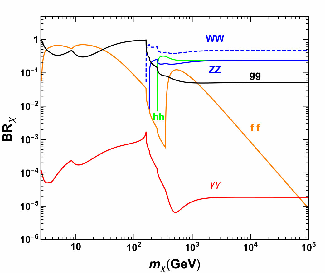 Figure 1
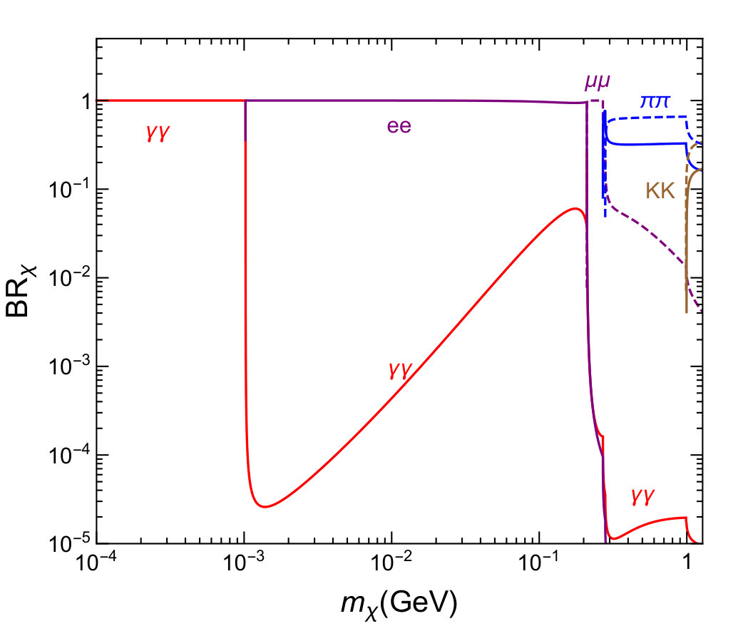 Figure 2
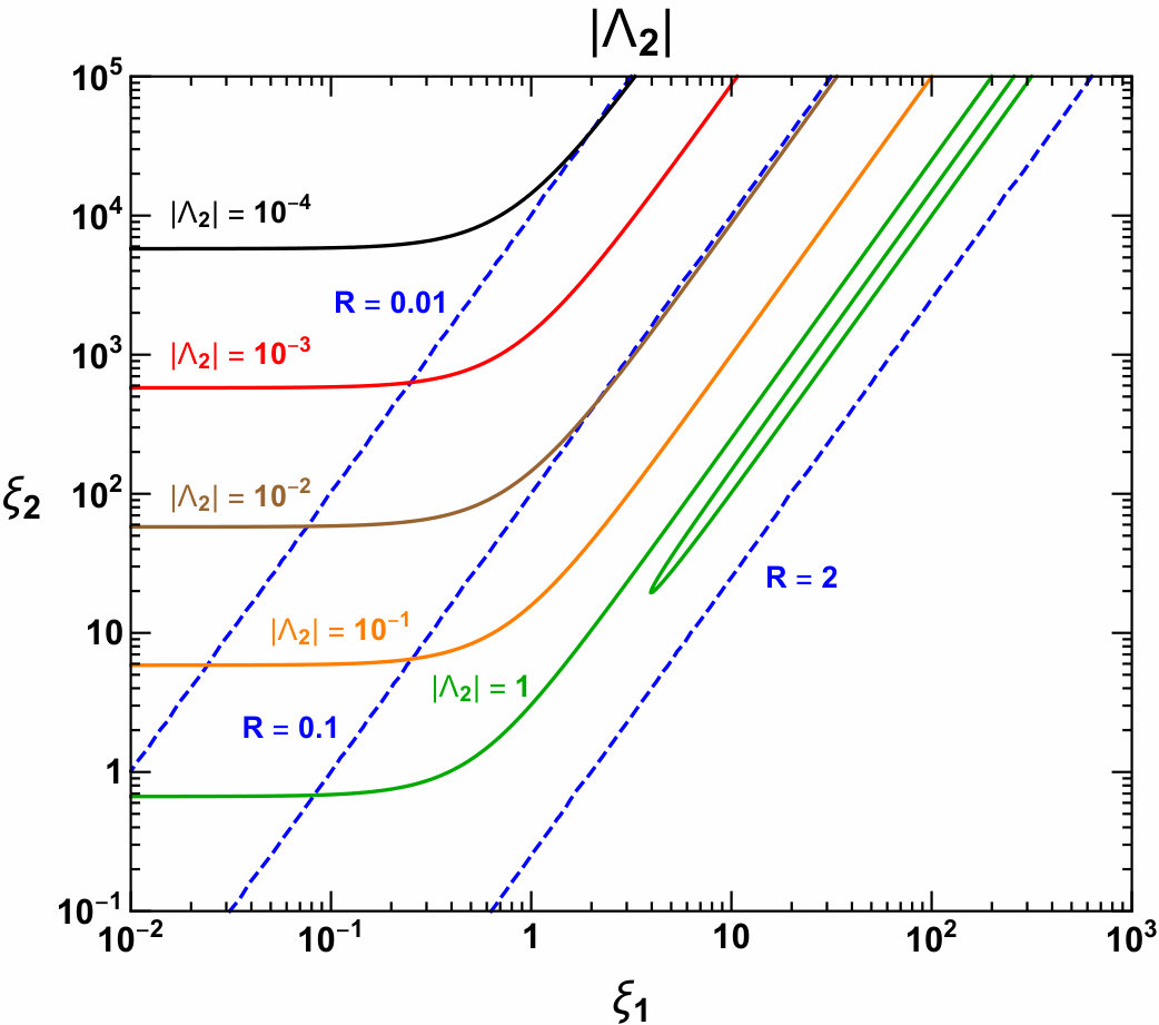 Figure 3
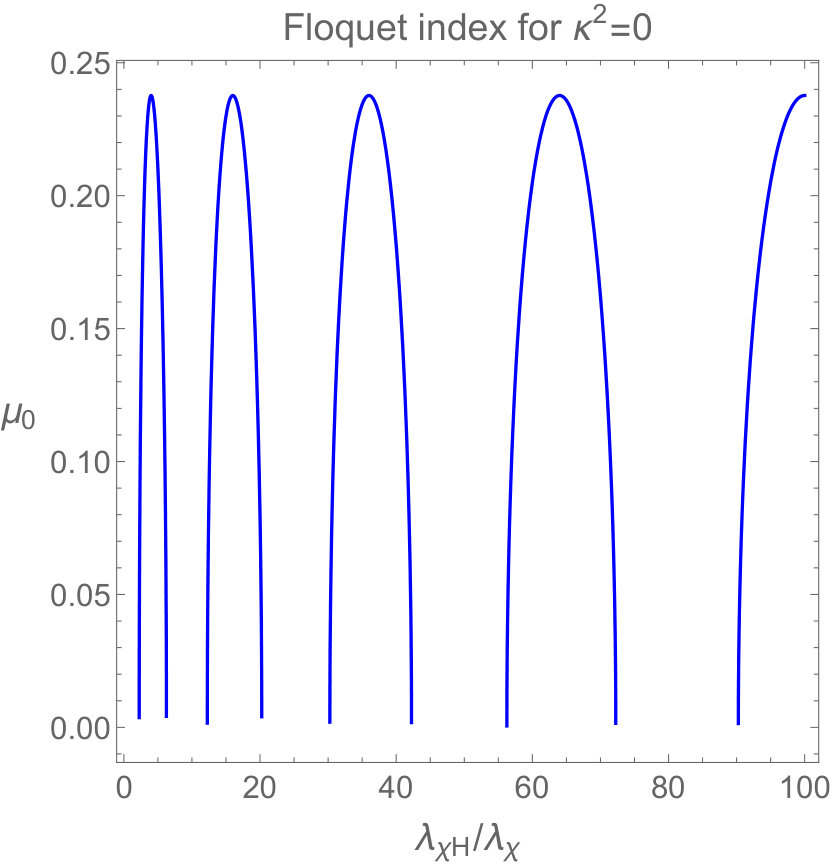 Figure 4
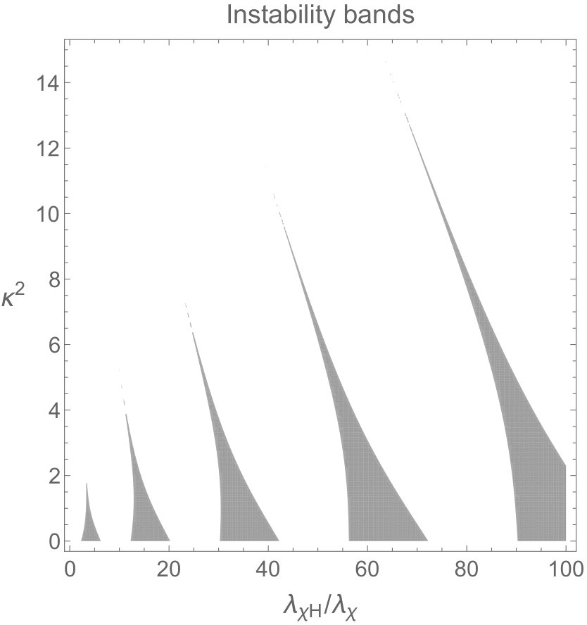 Figure 5
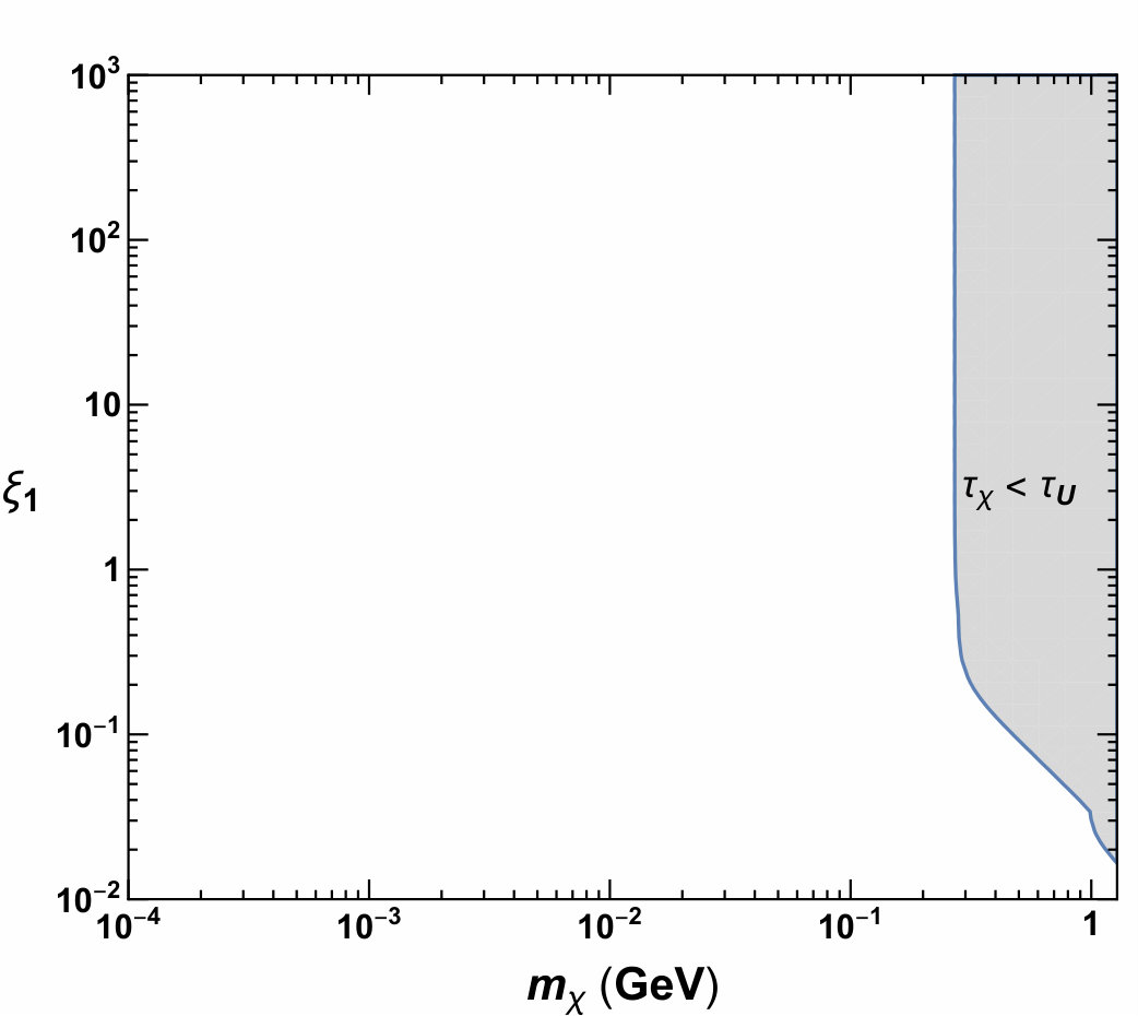 Figure 6
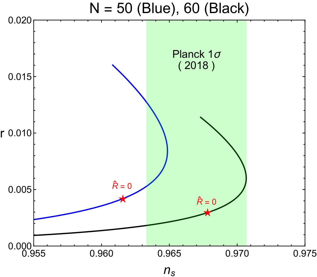 Figure 7
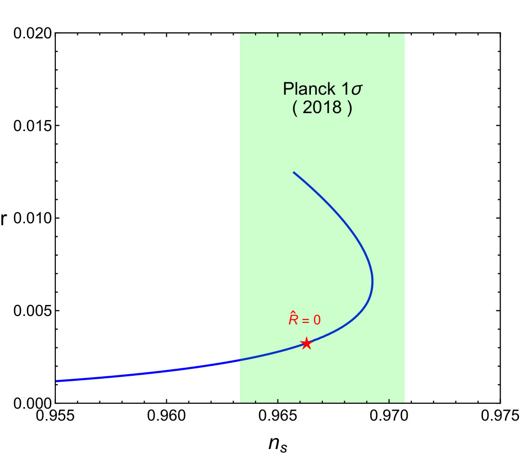 Figure 8
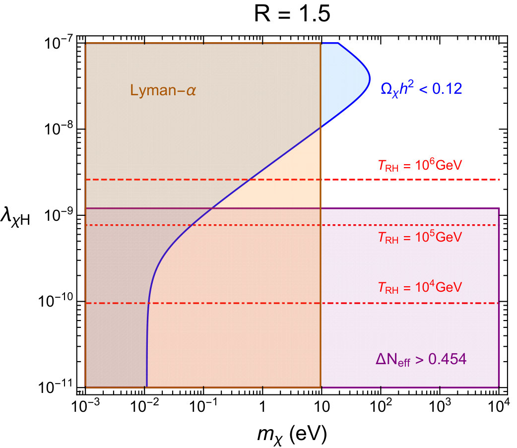 Figure 9
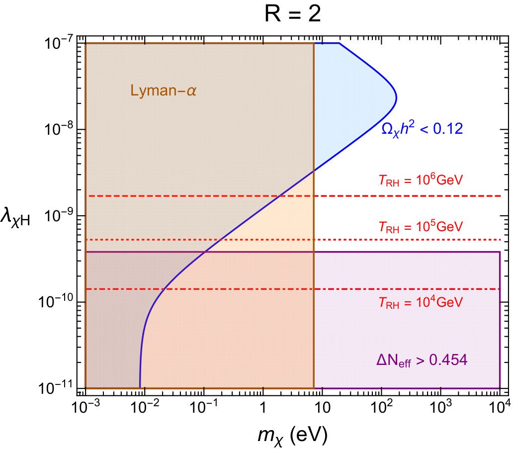 Figure 10
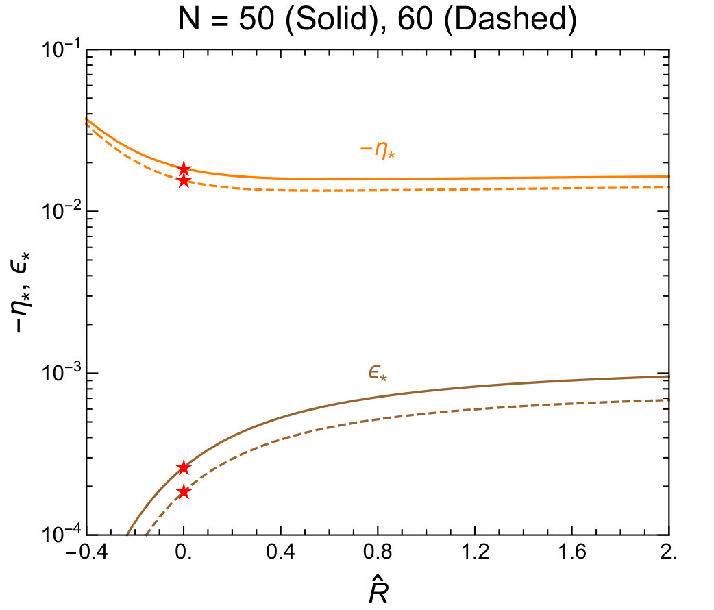 Figure 11
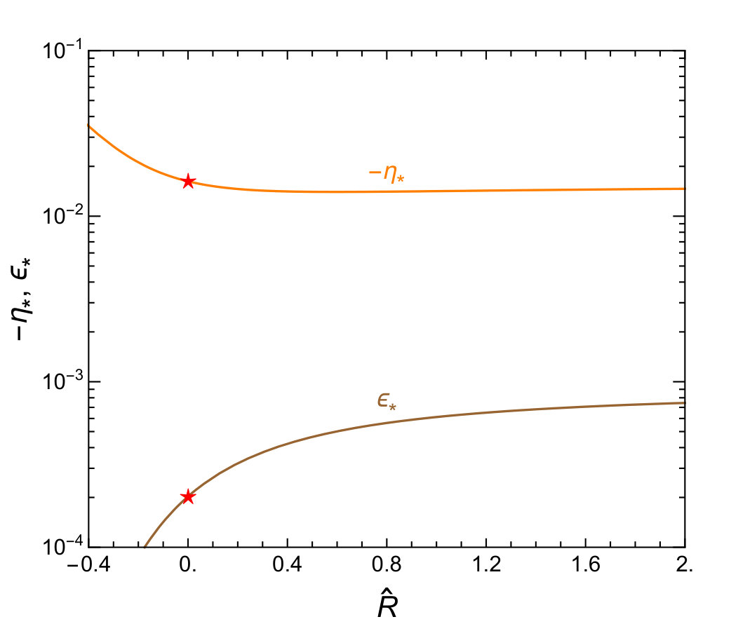 Figure 12
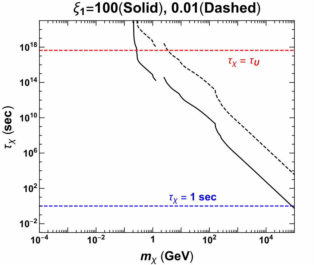 Figure 13
Peer Reviews
No public reviews on file for this paper yet. If you reviewed it on a platform where reviews are public (OpenReview, ICLR, NeurIPS, ICML), you can paste yours below so the community can read it here.
Videos
No videos yet. Explain this paper in a talk, walkthrough, or lecture? Add one.
{centering}
**Unitary inflaton as decaying dark matter **
**Soo-Min Choi1,†, Yoo-Jin Kang1,‡, Hyun Min Lee1,2,∗ and Kimiko Yamashita3,# **
1Department of Physics, Chung-Ang University, Seoul 06974, Korea.
2School of Physics, Korea Institute for Advanced Study, Seoul 02455, Korea.
3Department of Physics, National Tsing Hua University, Hsinchu, Taiwan 300.
We consider the inflation model of a singlet scalar field (sigma field) with both quadratic and linear non-minimal couplings where unitarity is ensured up to the Planck scale. We assume that a symmetry for the sigma field is respected by the scalar potential in Jordan frame but it is broken explicitly by the linear non-minimal coupling due to quantum gravity. We discuss the impacts of the linear non-minimal coupling on various dynamics from inflation to low energy, such as a sizable tensor-to-scalar ratio, a novel reheating process with quartic potential dominance, and suppressed physical parameters in the low energy, etc. In particular, the linear non-minimal coupling leads to the linear couplings of the sigma field to the Standard Model through the trace of the energy-momentum tensor in Einstein frame. Thus, regarding the sigma field as a decaying dark matter, we consider the non-thermal production mechanisms for dark matter from the decays of Higgs and inflaton condensate and show the parameter space that is compatible with the correct relic density and cosmological constraints.
†Email: [email protected]
‡Email: [email protected]
∗Email: [email protected]
#Email: [email protected]
1 Introduction
Measurements of anisotropies of Cosmic Microwave Background (CMB) provide important clues to the early Universe after Big Bang, such as inflation, dark matter and dark energy. In particular, it has been shown that the observed CMB spectrum [1, 2] is consistent with the predictions from the slow-roll inflation with a single canonical scalar field, the so called inflaton. However, what causes the inflation is unknown, although some of the early proposed inflation models including quartic or quadratic inflaton potentials have been now disfavored.
Higgs inflation [3] has been proposed as an economic implementation of inflation in particle physics, just with a single non-minimal coupling of Higgs field to gravity, so it has drawn a lot of attention from both particle physics and cosmology communities. Some time after the proposal, it was also noticed that a large non-minimal coupling necessary for a successful Higgs inflation causes unitarity problem much below the Planck scale [4]. However, Higgs inflation can be saved under the assumption that new physics entering at unitarity scale respects the approximate scale symmetry [5] or due to extra degrees of freedom fully recovering the unitarity up to the Planck scale [6, 7, 8, 9].
Recently, a new proposal for unitarizing Higgs inflation with a light inflaton, dubbed the sigma field , has been made by one of the authors [10]. In this case, the inflaton carries both quadratic and linear non-minimal couplings. As a result, we can keep the flat direction for inflation due to a large quadratic non-minimal coupling and, at the same time, unitarity scale is restored up to the Planck scale due to the field-independent rescaling of the inflaton field due to the linear non-minimal coupling. In this framework, the sigma field mass can take any value below the unitarity scale of the original Higgs inflation such that we can recover the Higgs inflation in the effective theory, but with a sizable correction to the tensor-to-scalar ratio at tree level.
In this article, we investigate the impacts of the linear non-minimal coupling on various dynamics from inflation to low energy phenomena such as reheating and inflaton couplings, in connection to unitarity scale and inflationary predictions. The symmetry for is respected by the inflaton potential in Jordan frame but it is broken explicitly by the linear non-minimal coupling. Then, the inflaton has novel couplings to the SM through the trace of the energy-momentum tensor with a suppression of the Planck scale in Einstein frame. In this case, we pursue the possibility that the inflaton can be a decaying dark matter (DM). To this, we consider the non-thermal production mechanisms for dark matter from the decays of the SM Higgs boson and the inflaton condensate. As a result, we show the parameter space for a decaying dark matter that is consistent with the correct relic density and cosmological constraints. There has been a recent proposal of axion-like inflation where the inflaton makes a decaying dark matter too [11].
The paper is organized as follows. We begin with a model description for the sigma field inflation and discuss the inflationary dynamics along the flat direction in the system with sigma and Higgs fields. Then, we continue to consider the reheating dynamics with a novel quartic potential and identify the possible reheating temperature depending on the mixing quartic coupling. Next we show how the unitarity is restored up to the Planck scale due to a sizable linear non-minimal coupling and identify the low energy parameters in the potential and inflation couplings to the SM through the trace of the energy-momentum tensor. As a result, the decay branching ratios of the inflaton are shown for heavy or light inflaton cases. Then, we show the parameter space for inflaton dark matter that is consistent with the correct relic density and the Big Bang Nucleosynthesis (BBN), CMB and large-scale structure bounds. Finally, conclusions are drawn. There is one appendix dealing with the details on inflaton decay rates.
2 Model
We consider the inflation model with a real scalar field as a simple extension of the Standard Model (SM), with the corresponding Lagrangian [10] being
[TABLE]
where the frame function and the scalar potential are given by
[TABLE]
We note that is the SM Higgs doublet, is to collectively describe the field strength tensors for the SM gauge bosons, and are the SM fermions, and and are covariant derivatives, , and is a constant term which is chosen to set the cosmological constant in the vacuum to zero. Here, we assume that the sigma field is odd under a symmetry, i.e. , that is respected by the scalar potential but broken only due to the linear non-minimal coupling in quantum gravity. As will be discussed later, it is still possible to make the inflaton as a decaying dark matter if light enough, even in the presence of the violation of the symmetry.
We note that the symmetry gets restored in the limit of a vanishing , so it is natural to introduce the approximate symmetry in the low energy. As will be shown in Sections 5 and 6, the breaking is communicated to the SM via gravitational interactions, thus it appears as higher dimensional interactions with suppression scales larger than or equal to the Planck scale in Einstein frame. Then, we can regarding our setup as an effective theory below the Planck scale. Therefore, as far as higher dimensional operators are suppressed by the Planck scale at least, our later discussion based on the breaking non-minimal coupling holds.
When the sigma field is heavier than electroweak scale, it is too short-lived to be a dark matter candidate. In this case, after integrating out a heavy sigma field with , we obtain a Higgs effective theory with the effective frame function and scalar potential [10], given by
[TABLE]
with
[TABLE]
Therefore, the effective Higgs quartic coupling gets a tree-level shift due to the scalar threshold, curing the vacuum instability problem in the SM[12, 13]. Moreover, a large positive effective non-minimal coupling for the Higgs field can be obtained and the effective frame function also contains a non-analytic form of the non-minimal coupling to gravity for the Higgs field, being proportional to the linear non-minimal coupling for the sigma field. However, we will fully take into account the sigma field in our later discussion and focus on the case with a light sigma field.
For , in order to maintain the effective Planck mass squared in Jordan frame to be positive during the cosmological evolution, we impose the condition for stable gravity [10] as
[TABLE]
with . Then, eq. (10) leads to the upper bound on the linear non-minimal coupling for stable gravity in the entire field space. We will take this into account in the later discussion on inflationary dynamics.
Choosing the Higgs doublet in unitary gauge as and performing the metric rescaling by with , we get the Einstein frame Lagrangian of our model as
[TABLE]
where are SM fermion and electroweak gauge boson masses, independent of the sigma field, and for bosons, and the Einstein frame potential is given by
[TABLE]
with
[TABLE]
Here, we note that the SM fermions are rescaled by for canonical kinetic terms in eq. (11) and the form of covariant kinetic terms for fermions is unchanged under the Weyl transformations of the metric and fermions.
From the following,
[TABLE]
and the Einstein frame Lagrangian given in eq. (11), the scalar kinetic terms in Einstein frame can be rewritten as
[TABLE]
We will make use of the above form of the kinetic terms for our later discussion on inflationary dynamics and unitarity scales in the true vacuum.
Furthermore, from eq. (11), we also note that the inflaton couplings to the SM in Einstein frame can be read from
[TABLE]
The above interaction Lagrangian will be useful for discussing the reheating dynamics and inflation couplings at low energy in the later sections.
3 Inflationary dynamics
We consider the inflationary dynamics in our model with sigma and Higgs fields along the flat direction and discuss the details of the vacuum structure during inflation. After obtaining the effective potential for a single inflaton, we show the differences from the usual inflation with quadratic non-minimal couplings only.
3.1 Inflaton dynamics along the flat direction
Taking during inflation, we get and introduce a new set of fields [10] by
[TABLE]
Then, from the approximate relation between and redefined fields, and , given by
[TABLE]
with
[TABLE]
the scalar potential in Einstein frame111We have corrected the typo in the last term of the scalar potential in Ref. [10]: . becomes
[TABLE]
with
[TABLE]
Thus, the ratio of the fields is determined dominantly by the minimization of with respect to . We note that for , i.e. for zero during inflation, is identical to , that will appear in the unitarity scales in Section 5. We note that the value of is constrained to for stable gravity [10], as discussed for eq. (10).
Now we discuss the scalar kinetic terms in Einstein frame and check the consistency of the inflaton identification in the above discussion. First, we can rewrite eq. (15) in terms of the shifted sigma field, , as
[TABLE]
Here, during inflation, we can ignore in eq. (23) so the kinetic terms are essentially the same as in the sigma field inflation without the linear non-minimal coupling, although there is a significant difference in the vacuum as will be shown in the later sections.
In the basis of and , the Einstein-frame kinetic terms in eq. (23) are generically non-diagonal [14, 15, 10]. Thus, we have to choose another basis with , instead of , as follows,
[TABLE]
This is the Noether current of scale symmetry [16, 17], which is approximately respected during inflation because is close to a constant value up to small slow-roll parameters. Redefining the scalar fields in terms of and [18, 17] as
[TABLE]
we find that the above Einstein-frame kinetic terms in eq. (23) become diagonal,
[TABLE]
This is a more convenient form for discussing the inflaton effective potential with the field decoupled in the next section.
3.2 Effective action for inflaton
After stabilization of from the scalar potential in eq. (22), we get four different vacua for during inflation and the corresponding minimum conditions [14], in the following,
[TABLE]
Then, there is a unique vacuum for in the first three cases, and the vacuum energy in each case given [14] by
[TABLE]
whereas there are two local minima in the last case (4), with the same vacuum energy as given in the cases (2) and (3), respectively.
In the case with and quartic couplings of order unity, the conditions for the inflation vacua (28) become
[TABLE]
In the first two cases, we need the Higgs quartic coupling to be positive during inflation: the former is the sigma-Higgs mixed inflation and the latter is the pure sigma inflation. In the third case, as the Higgs quartic coupling is required to be negative as , , so it is not possible to get a dS vacuum for inflation. Finally, in the fourth case, even for , the inflation could be driven by the sigma field at the metastable vacuum with so it could lead to a viable cosmology with correct electroweak symmetry breaking at low energy. But, is not a valid option because the vacuum energy during inflation is negative, i.e. . The vacuum energy (29) for the viable inflation is given by
[TABLE]
Therefore, for and (or ) stabilized at (or ), the Einstein-frame kinetic terms in eq. (27) become simplified to
[TABLE]
Here, we note that since
[TABLE]
where
[TABLE]
the above result with the canonical inflaton field is consistent with eq. (17).
In summary, from eqs. (32) and (21), the approximate Einstein-frame Lagrangian for inflation is given [10] by
[TABLE]
with
[TABLE]
We note that the physical mass for the field is rescaled by the non-minimal coupling to , which is much larger than the Hubble scale during inflation, so we can safely ignore the dynamics of the field for the inflationary dynamics.
3.3 Inflationary predictions
From the effective inflaton Lagrangian in eq. (35), the slow-roll parameters during inflation are given approximately by
[TABLE]
As a result, the spectral index is given by
[TABLE]
where denotes the evaluation of the slow-roll parameters, (37) and (38), at horizon exit. The tensor-to-scalar ratio is also given by with eq. (37) at horizon exit. We note that the measured spectral index and the bound on the tensor-to-scalar ratio are given by and at C.L., respectively, from Planck 2018 (TT, TE, EE + low E + lensing + BK14 + BAO) [2], as compared to and at C.L. in Planck 2015 (TT, TE, EE + low P) [1]. Thus, the experimental errors in the spectral index from Planck 2018 combination are reduced a bit but the central value of the spectral index is consistent with the one from Planck 2015.
Moreover, with eq. (37), the number of efoldings required to solve the horizon problem can be calculated as follows,
[TABLE]
with
[TABLE]
where are the inflaton values at the beginning and end of inflation and we can take . Then, we can solve eq. (40) for to express the slow-roll parameters at horizon exit in terms of the number of efoldings and .
In Fig. 1, we show the slow-roll parameters as a function of for and in solid and dashed lines, respectively, on left, and for in the case with perturbative reheating, on right. The parameter is sensitive to the value of , increasing as gets larger. Moreover, in Fig. 2, we depict the predictions for the spectral index and the tensor-to-scalar ratio in our model for and in blue and black lines, respectively, on left, and for in the case with perturbative reheating, on right. The values of are taken between and . In the presence of a sizable , the region compatible with Planck 2018 data is enlarged and the tensor-to-scalar ratio is as large as , which is at the detectable level in future CMB experiments.
For , i.e. , the results with quadratic non-minimal couplings only are recovered, namely, , and . Then, we get and , so the spectral index and the tensor-to-scalar ratio become and , respectively [3].
Finally, from the normalization for CMB anisotropies, the vacuum energy during inflation is constrained by at the Planck pivot scale of [2]. Then, for and , depending on the viable inflation vacua given in (31), we need the combination of quartic couplings and the quadratic non-minimal coupling to satisfy the following conditions,
[TABLE]
Therefore, in the case with sigma-Higgs mixed inflation (1), there is a cancellation between quartic couplings, so the CMB normalization can be satisfied for a relatively smaller . On the other hand, in the case with sigma inflation (2), (4), the non-minimal coupling must be very large unless is small.
4 Reheating
In order to discuss the reheating process, we need to identify the form of the inflaton potential at the onset of inflaton oscillation near the minimum. We show that the sigma-field potential becomes quartic already at the end of inflation due to a sizable linear non-minimal coupling, so the reheating dynamics becomes different from the usual inflation without a linear non-minimal coupling. We also obtain the reheating temperature of our model, depending on the mixing quartic coupling between sigma and Higgs fields. Then, we discuss the relevance of preheating and the instability regions for quartic couplings in our model.
4.1 Inflaton potential during reheating
For simplicity, we focus on the reheating process of the pure sigma-field inflation but a similar discussion applies for the mixed inflation. With during inflation, from eq. (11) or (15), the canonical inflaton field is related to the original sigma field by
[TABLE]
with . Therefore, as far as , we always get , so the above equation becomes simplified, independent of field values, to
[TABLE]
Thus, we obtain the canonical inflaton field as
[TABLE]
or
[TABLE]
with .
As a result, we obtain the inflaton potential in Einstein frame, as follows,
[TABLE]
Then, we can recover the approximate inflaton potential (21) with during inflation for or . On the other hand, after the end of inflation, i.e. , we can expand eq. (47) to get the inflaton potential during reheating as follows,
[TABLE]
Consequently, we find that the inflaton potential becomes quartic during reheating, due to a sizable linear non-minimal coupling. In this case, the effective quartic coupling for the inflaton becomes suppressed by . The suppressed quartic coupling is due to the redefined sigma field with near the true vacuum, as will be discussed in more detail in the next section.
For comparison, when or as in Higgs inflation [19], the inflaton potential (47) becomes
[TABLE]
The above potential is valid for , so the inflaton potential becomes quadratic as during reheating [19], unlike the case with . Moreover, from eq. (43), when , eq. (43) with leads to , thus the sigma-field potential becomes the same as the one in Jordan frame as , without a suppression of the quartic coupling.
4.2 Decays of inflaton condensate and reheating temperature
In the presence of the quartic inflaton potential during reheating, the inflaton background field (or condensate) evolves in time [21, 23], as follows,
[TABLE]
Here, {\rm cn}\Big{(}\omega(t)\,t,\frac{1}{\sqrt{2}}\Big{)}\approx\cos(0.85\omega(t)) with being the oscillation frequency of the inflaton with , and the amplitude of oscillation is given by with . We note that is the Jacobi cosine for .
From eq. (16), we consider the relevant Lagrangian for reheating, composed of the inflaton quartic potential and the inflaton interactions in Einstein frame, as follows,
[TABLE]
where and is used, and is the gravitational inflaton interaction from eq. (16) during reheating, due to the frame function with eq. (45), given by
[TABLE]
Then, from the quartic terms in the potential in eq. (51), the inflaton and Higgs boson particles have background-dependent masses due to the inflaton condensate as
[TABLE]
where are inflaton-independent scalar masses. As a result, the decay width of the inflaton condensate [23] is determined to be
[TABLE]
with
[TABLE]
We note that the gravitational contributions to and additional decay modes can be ignored as far as or . Henceforth, we assume that this is the case, as will be shown in the later section.
Then, from the condition for the inflaton decoupling at , for which
[TABLE]
with
[TABLE]
we obtain the amplitude of the inflaton condenstate as
[TABLE]
Therefore, under the condition of instantaneous reheating,
[TABLE]
with eq. (60), we get the reheating temperature as
[TABLE]
with
[TABLE]
Here, we used from the CMB normalization in eq. (42). Therefore, for and , choosing , we get and .
4.3 Preheating from Higgs portal coupling
Preheating is a non-perturbative process for reheating and it becomes sometimes dominant. In our case, since the effective mass of Higgs boson depends on the time-dependent inflaton condensate, this leads to the non-adiabatic excitation of the Higgs perturbation by parametric resonance [20, 21, 22].
As discussed in the previous subsection, the inflaton potential becomes quartic during reheating, so the inflaton condensate follows eq. (50). Then, the Fourier mode of the Higgs perturbation with comoving momentum satisfies the following modified Klein-Gordon equation [21],
[TABLE]
Then, redefining the Higgs perturbation by and introducing the conformal time by , we can write eq. (64) [21] as the Lamé equation,
[TABLE]
where the prime denotes the derivative with respect to the conformal time , and , and the comoving momentum in units of the initial effective mass of the inflaton is given by
[TABLE]
Here, we ignored the inflation-independent Higgs mass, , in eq. (54). Then, the number of Higgs particles created during preheating grows exponentially as with a Floquet index . When , with being the Higgs decay rate, preheating works for Higgs production. From with being the bottom Yukawa coupling, the condition for preheating to work for Higgs production is
[TABLE]
Here, we note that both and are proportional to , unlike the case with the quadratic inflaton potential where is replaced by the inflaton mass, so preheating rate exceeds the Higgs decay rate only if eq. (67) is fulfilled. On the other hand, if , i.e. outside the instability bands, preheating can be ignored.
Furthermore, preheating can be dominant over perturbative reheating, provided that with eq. (55), that is,
[TABLE]
Therefore, as far as preheating is efficient according to eq. (67), it would become a dominant process for reheating. We note that from , eq. (68) is equivalent to . If eq. (68) is satisfied, the reheating temperature can be determined approximately by the condition, , where is the Hubble parameter during reheating. In this case, the resulting reheating temperature can be much larger than the one determined by perturbative decay in the previous subsection.
In the case of , which is our interest for the later discussion on decaying dark matter, we expand {\rm cn}\Big{(}x,\frac{1}{\sqrt{2}}\Big{)}\approx x near . Then, it can be shown that the equation for the Floquet index is given [21] by
[TABLE]
where is the period of the oscillations in units of , and , and the phase is approximated to
[TABLE]
Then, there exists a solution to eq. (69), i.e. the exponential growth of created particles is possible, only if
[TABLE]
On the left in Fig. 3, we show the instability bands for preheating in the parameter space for and the comoving momentum . On the right in Fig. 3, for zero momentum mode, we draw the Floquet index as a function of , with its maximum being given by . As a consequence, in the region where eq. (71) is satisfied, preheating is efficient enough to determine the reheating temperature at a higher value as compared to the case with perturbative decays.
Preheating process becomes important for broad resonances near the zero momentum mode on the left in Fig. 3. However, in the narrow resonances close to cuspy ends of each instability band in the same plot, the redshift of momenta away from the resonance band can prevent parametric resonance from being efficient [20]. Then, we can estimate the condition for preheating into the Higgs perturbation to be dominant as where is the width of the narrow resonance. Therefore, the original condition with broad resonances in eq. (68) is generalized to . Therefore, for a sufficiently small , we can ignore preheating safely but instead rely on the perturbative decays of the inflaton for reheating, as discussed in the previous subsection. We assume that this is the case for our later discussion for the calculation of dark matter abundance from the inflaton.
Before ending this subsection, we comment on the inflaton perturbation and preheating. The corresponding Lamé equation for with the inflaton perturbation is
[TABLE]
Here, we also ignored the bare inflaton mass, , in eq. (53). In this case, the inflaton perturbation grows for the momenta in the range, [21]. However, the modes of the inflaton perturbations which are amplified are at sub-Hubble scales during reheating [22], so there is no effect of the inflaton perturbations produced from preheating at large scales such as CMB [22]. The maximum growth for is at [21]. If the inflaton perturbation is decoupled from the SM due to small couplings, i.e. , the produced inflaton would not thermalize the SM particles.
5 Non-minimal couplings and unitarity scales
We discuss the impacts of the linear non-minimal coupling in identifying the physical parameters of the scalar potential in the vacuum and show how the unitarity problem with a large quadratic non-minimal coupling can be eliminated by an appropriate linear non-minimal coupling.
5.1 Physical parameters in the vacuum
Taking near the vacuum, we get the approximate quadratic kinetic terms in eq. (15) as
[TABLE]
Then, from the canonical sigma field,
[TABLE]
the frame function becomes
[TABLE]
Moreover, we get the Einstein-frame potential (12) for the canonical sigma field , as follows,
[TABLE]
with
[TABLE]
On the other hand, the interaction terms containing only do not rescale. Therefore, if dimensionful and dimensionless parameters are of common origin in Jordan frame, we can get a natural hierarchy of masses and couplings for : , and .
After electroweak symmetry breaking, the effective mass of the inflaton has a tree-level shift as , due to the mixing Higgs quartic coupling. Higgs loop corrections to the inflaton mass is , so they are subdominant as compared to the tree-level shift. The mass shift of the inflaton is much smaller than the Higgs mass for ,. In a later discussion for light inflaton dark matter, however, we need to tune the bare inflaton mass against for a phenomenologically desirable mass, such as for the relic density. For simplicity, henceforth we use the same notation for the effective inflaton mass as .
5.2 Unitarity scales
In terms of the canonical sigma field, we obtain the leading derivative interaction terms [10] from eq. (15),
[TABLE]
where the ellipses are higher dimensional terms and the cutoff scales in the leading terms read
[TABLE]
with
[TABLE]
Here, we assumed in the above approximations. For and , the unitarity scales depend only on the ratio of the non-minimal couplings, . In Fig. 4, as a representative example, we draw the contour plot for the unitarity scale in the parameters space for and , showing that is saturated to in order to maintain of order the Planck scale for a large .
6 Inflaton couplings to the SM at low energies
The sigma field also has dilaton-like couplings to the SM through the trace of the energy-momentum tensor, due to the linear non-minimal coupling. In this section, we consider all the linear couplings of the sigma field to the SM in the low energy in Einstein frame.
From and eq. (76), we expand the inflaton interaction Lagrangian (16) in Einstein frame to identify the linear coupling of the canonical sigma field as follows,
[TABLE]
where is the trace of the energy-momentum tensor at tree level on the equations of motion and use is made of the canonical sigma field (74) in the true vacuum. Here, we have recovered the Planck scale , and is given in units of .
We remark that the minimal couplings of gauge bosons to SM fermions do not depend on the frame function , so there is no coupling between the sigma field and one SM gauge boson. Since the covariant derivative terms of fermions do not contribute to the trace of the energy-momentum tensor, our results confirm that minimal couplings between the sigma field and one SM gauge boson are absent, unlike the approach of Ref. [28] where these couplings however arise at higher orders in perturbation theory.
6.1 Inflaton couplings to massive particles
From eq. (90), we consider the linear couplings of the sigma field to the Higgs field,
[TABLE]
The tadpole term for vanishes in the vacuum with a vanishingly small cosmological constant, , leading to an extremely tiny VEV of the sigma field, thus the Higgs-sigma mixing is negligible. Thus, this is different from the case where a light inflaton carries a sizable Higgs mixing due to a sizable inflaton VEV so it has Higgs-like couplings to the SM [24]. Moreover, the mass mixing vanishes in the minimum of the potential . We note that the effective mass of the sigma field is shifted to after electroweak symmetry breaking, but we keep the same notation for the sigma field mass as for simplicity.
As a consequence, expanding the Higgs field about the vacuum as , the linear couplings of the sigma-like field (91) become
[TABLE]
Then, the sigma field decays into a pair of Higgs bosons, on-shell or off-shell, through the Higgs kinetic term and mass term. We note that the Feynman rule for the vertex with one sigma field and two Higgs bosons with outgoing momenta, and , is given by
[TABLE]
From eq. (90), with , we get the linear couplings of the sigma field to massive fermions and electroweak gauge bosons as
[TABLE]
Then, the sigma field can decay into a pair of SM fermions or gauge bosons. If the sigma field is lighter than pions, it can decay dominantly into a pair of muons for or a pair of electrons for .
6.2 Inflaton couplings to massless gauge bosons
We now consider the sigma field couplings to massless gauge bosons. In this case, there are two contributions coming from trace anomalies and threshold effects due to heavy particles.
First we note that the trace of the energy-momentum tensor is corrected due to scale anomalies at loop order to the following,
[TABLE]
where and are the beta functions for and , respectively, and they are given at one loop by and where are beta function coefficients in the SM, given by and , respectively. Therefore, with in eq. (90) being replaced , there are sigma field couplings to two photons and two gluons.
Furthermore, the sigma field couples to massive particles through the energy-momentum tensor in . Since all the SM particle have sigma-field dependent masses, , where being independent of the sigma field, they contribute to the effective QED gauge coupling at the threshold, , as
[TABLE]
with is the cutoff scale and is the QED gauge coupling at the cutoff scale. Therefore, from the gauge kinetic term, , after absorbing the gauge coupling by the gauge field with , we obtain the additional contributions to the effective sigma field coupling to photons, as follows,
[TABLE]
where the beta function coefficient for EM gauge coupling is given by
[TABLE]
with and . Here, the sum is performed over all the SM charged fermions heavier than the typical energy scale, for instance, the inflaton mass, in case of the inflaton decay process. For example, for , ; for , ; for , . For , it decays dominantly into a photon pair.
Consequently, including the sigma field coupling due to trace anomalies in eq. (96), we obtain the full effective sigma field coupling to photons as
[TABLE]
with being the beta function coefficient for EM gauge coupling due to light charged particles. Thus, the contributions from heavy charged particles cancel the counterpart of scale anomalies, leaving the scale anomalies from light charged particles.
Similarly, the threshold corrections to the running QCD gauge coupling due to heavy quarks lead to the additional contribution to the sigma field couplings to gluons, as follows,
[TABLE]
where is the QCD beta function coefficient due to heavy quarks, given by . Consequently, including the sigma field coupling due to trace anomalies in eq. (96), we obtain the full effective sigma field coupling to photons as
[TABLE]
with being the beta function coefficient for strong gauge coupling due to light quarks and gluons. Thus, similarly to the case with photon couplings, there is a cancellation between the contributions from heavy colored quarks and the counterpart of scale anomalies, so the scale anomalies from light quarks and gluons remain.
If the sigma field is heavier than , we can consider the sigma field decays into a gluon pair. But, for , either descriptions in terms of mesons or quarks/gluons are not quite correct [25]. For , we can use the description of quarks/gluons and the coefficient of the QCD beta function, which is given by from light quarks only.
We note that the effects of heavy particle masses in the effective inflaton couplings to photons and gluons, and , can be taken into account through the loop functions as shown in eqs. (A.4) and (A.5) of the appendix.
6.3 Inflaton couplings to mesons
When the sigma field is lighter than , we need to include the sigma field decays into a pair of mesons in chiral perturbation theory, instead of quarks or gluons. In this case, we need to take the beta function coefficient of strong gauge coupling as for for light quarks in chiral perturbation theory [30].
From eqs. (90) and (102), we consider the relevant interactions of the sigma field to light quarks and gluons in the low energy as
[TABLE]
with . Then, using PCAC relation, , we obtain the linear couplings of the sigma field to mesons as
[TABLE]
which is nothing but the coupling to the trace of energy-momentum tensor for mesons. Thus, the Feynman rule for the vertex with one sigma field and two pions with outgoing momenta, and , is given by
[TABLE]
For instance, for the decay of the sigma field into a pair of pions, we get .
In Fig. 5, we show the decay branching ratios of the inflaton in the cases of light inflaton below on left and heavy inflaton above on right. Formulas for inflaton decay rates are collected in the appendix. In the case of light inflaton, the inflaton decays into muons, pions or kaons above the muon threshold while it decays dominantly into an electron pair below the muon threshold but above the electron threshold. On the other hand, in the case of heavy inflaton, the inflaton decays dominantly into gluons or fermion pairs below the threshold, while it decays dominantly into the electroweak sector, , above the threshold.
7 Long-lived inflaton as dark matter
We consider the sigma field or inflaton as a decaying dark matter and show the parameter space for the correct relic density of the long-lived dark matter, based on Feebly Interacting Massive Particle (FIMP) process after reheating as well as the decays of the inflaton condensate during reheating.
7.1 Long-lived inflaton
As soon as the decay of the sigma field into a pion pair opens up, the lifetime of the sigma field would be less than the age of the Universe, independent of for . Therefore, in most of the parameter space, the sigma field can be a candidate for dark matter only for [28]. This fact is shown on the left of Fig. 6, in the gray region of the parameter space for vs where the inflaton does not survive until the present Universe. On the right of Fig. 6, we also draw the contours of the inflaton lifetime as a function of for in black solid and dashed lines, respectively. We find that the inflaton lifetime ranges between the age of the Universe and for with , as shown from the lines with and .
Dark matter can be in thermal equilibrium, as far as or for . But, dark matter can annihilate into a pair of muons or electrons for . For instance, the cross section for the annihilation, , is suppressed by the SM Higgs mass and the muon Yukawa coupling, as follows,
[TABLE]
On the other hand, the necessary annihilation cross section for thermal freeze-out is with the effective DM coupling being given by for . However, this condition is not satisfied in our model, so we need to rely on non-thermal production mechanisms.
7.2 Relic density from FIMP inflaton
For a small mixing quartic coupling between the sigma field and Higgs boson, i.e. , the sigma field could never be in thermal equilibrium. Thus, the total relic density of inflaton dark matter is determined by two non-thermal mechanisms, as follows,
[TABLE]
One is the FIMP contribution [26], generated by Higgs decay at the temperature . The other is the contribution from the decay of the inflaton condensate during reheating [23].
First, in the presence of a nonzero , the Higgs decay into a pair of sigma fields governs the DM relic density dominantly below the reheating temperature, as follows,
[TABLE]
where the Higgs decay rate is given by
[TABLE]
the equilibrium number density of Higgs is with in the non-relativistic limit, and the second term on right is the inverse decay term, which can be neglected for a small initial abundance of dark matter. Then, for , eq. (108) can be solved for as
[TABLE]
with and , which agrees well with the result from the exact thermal average [26]. Therefore, the relic density coming from the FIMP process is given by
[TABLE]
Next we consider the relic density of inflaton dark matter produced from the decay of the inflaton condensate during reheating. The energy density of dark matter at the decoupling is given by
[TABLE]
where BR is the branching ratio of the inflaton condensate decaying into a pair of inflatons in eq. (59). Then, at the decoupling, dark matter has the peak energy at and it becomes non-relativistic when at due to the redshift of the momentum. Assuming that dark matter becomes non-relativistic before matter-radiation equality for structure formation, the energy density of dark matter at matter-radiation equality is given by
[TABLE]
First, using eq. (58), we obtain the red-shift factor at the time when dark matter becomes non-relativistic as
[TABLE]
Then, assuming that there is no entropy change between decoupling and matter-radiation equality, we also get
[TABLE]
where , , , and . Therefore, using the above results and , we obtain eq. (113) with eq. (112) explicitly as
[TABLE]
Consequently, we get the general formula for the relic density coming from the reheating process as
[TABLE]
where the critical density at present is given by , , and in the last line, we used eq. (42) and . In the case that inflation reheats the SM particles dominantly, i.e. , the above relic density becomes
[TABLE]
Furthermore, from eqs. (114) and (115), we obtain the temperature ratios of at matter-radiation equality to at which dark matter becomes non-relativistic, as follows,
[TABLE]
Here, for and , we find that is greater than for , which is not favored by the correct relic density, as will be discussed shortly.
In the case with , dark matter is still relativistic during BBN, so we need to check the contribution of dark matter to the number of relativistic species, . Assuming that dark matter is still relativistic during BBN and using eq. (113), we get the DM relic density for as
[TABLE]
Then, from and \Delta\rho=\frac{\pi^{2}}{30}\cdot\frac{7}{4}\Big{(}\frac{4}{11}\Big{)}^{4/3}(\Delta N_{\rm eff})\,T^{4}, we obtain from dark matter during BBN as follows,
[TABLE]
where the inequality comes from , and we took for . The combined results of primordial abundance measurements of helium and deuterium and the CMB measurement by Planck constrain to be in case a), in case b), or in case c), depending on the computed deuterium fraction [2]. Therefore, our inflaton dark matter is consistent with such BBN constraints, as far as within in case c), for , and .
In Fig. 7, we show the parameter space for the DM relic density due to non-thermal production mechanisms in light blue region for and , for , on left and right plots, respectively. Using the reheating temperature obtained in eq. (62), we also indicate the contours with reheating temperature, , on left(right), in red dashed, dotted, dot-dashed (and solid) lines, respectively. Moreover, the light orange region is excluded by the bounds on the free-streaming length up to , from the Lyman- forest data [31] and the phase space densities derived from the dwarf galaxies of the Milky way [32]. Finally, purple region is with , which is beyond the limit of the BBN constraint in case c).
As a result, we find that light dark matter with is favored for the correct relic density, being compatible with BBN and CMB constraints. As the decay branching fraction of the inflaton condensate into an inflaton pair gets larger, the relic density becomes almost independent of the inflaton-Higgs quartic coupling, , and the reheating temperature gets smaller. But, the region with a large is disfavored by BBN constraints. On the other hand, for for , the inflaton condensate decays dominantly into a Higgs pair, so the relic density is saturated along the line with constant , as expected from the approximate formula in eq. (118).
We remark briefly on other potential constraints on the inflaton dark matter. We note that there is no mixing between Higgs and sigma fields in our model so there is no direct constraint on the mixing quartic coupling, , in the relevant parameter space for the correct relic density, and indirect constraint from Higgs invisible decays into a pair of sigma fields is not sensitive enough to bound such a tiny coupling. Furthermore, there are couplings of the sigma field to photons through the trace of the energy-momentum tensor in eq. (100) but such couplings are suppressed by the Planck scale, so there is no constraint from SN1987A or horizontal branch cooling [33] or fifth-force experiments [34]. On the other hand, the bounds from isotropic diffuse gamma-ray spectrum and CMB measurements [28] can constrain the parameter space for a decaying dark matter heavier than , but there is no constraint in the parameter space for FIMP dark matter in our model. There are also interesting constraints by electron absorption from XENON10 [35] on the detection of a light dark matter below or proposed experiments with superconductors or semi-conductors [36], but the sensitivity has not reached yet to probe our inflaton dark matter.
8 Conclusions
We have studied the dynamics of inflation models of a singlet scalar field with both quadratic and linear non-minimal couplings. Although the quadratic non-minimal coupling determines the flat direction for inflation, the linear non-minimal coupling starts to dominate already during reheating and rescales the effective quartic couplings and mass of the inflaton to small values. We identified the reheating temperature in this model and obtained the correct abundance of the inflaton dark matter by non-thermal production mechanisms with the decay of the inflaton condensate during reheating and the decay of Higgs after reheating.
It is intriguing that the inflaton couples to the trace of the energy-momentum tensor so does it to the full Jordan frame potential. As a result, there is no mixing between the inflaton and the SM Higgs boson in the vacuum, allowing for a definite prediction for the inflaton decay rates in terms of the linear non-minimal coupling and the inflaton mass. We showed that the effective quartic coupling of the inflaton is fixed by the CMB normalization while a tiny mixing quartic coupling between the inflaton and the SM Higgs boson can be varied to saturate the relic density for DM masses between and , being compatible with BBN, CMB and large-scale structure constraints.
Acknowledgments
We thank Fedor Bezrukov, Cristiano Germani, Pak Hang Chris Lau, Wan-Il Park and Chang Sub Shin for their valuable comments and discussions. HML appreciates fruitful discussions with participants during the CERN-CKC Theory Workshop on Scale Invariance in Particle Physics and Cosmology. The work of SMC, HML and YJK is supported in part by Basic Science Research Program through the National Research Foundation of Korea (NRF) funded by the Ministry of Education, Science and Technology (NRF-2016R1A2B4008759 and NRF-2018R1A4A1025334). The work of KY is supported in part by National Center for Theoretical Sciences. The work of SMC is supported in part by TJ Park Science Fellowship of POSCO TJ Park Foundation. The work of YJK is supported in part by the Chung-Ang University Graduate Research Scholarship in 2018.
Appendix A: Inflaton decay rates
The sigma inflaton field has couplings to the SM particles through the trace of the energy-momentum tensor. Here, we list formulas for the most relevant two-body decay rates of the inflaton, as follows [29, 30, 25],
[TABLE]
Here, for bosons, are the beta function coefficients of , and gauge couplings, given by in the SM, leading to for the beta function of EM gauge coupling, , , and the loop functions are given by
[TABLE]
where
[TABLE]
In the limit of decoupled particles, the loop functions are approximated to and for , thus recovering the low energy couplings coming from trace anomalies due to light particles only: in eq. (100) and in eq. (102).
For simplicity, we took the notations, , for the SM particle masses that are independent of the inflaton field value.
For , we need to rely on chiral perturbation theory to obtain the decay rates of the inflaton into a meson pair, as follows [25],
[TABLE]
The reference list from the paper itself. Each links out to its DOI / PubMed record.
- 1[1] P. A. R. Ade et al. [Planck Collaboration], Astron. Astrophys. 594 (2016) A 20 doi:10.1051/0004-6361/201525898 [ar Xiv:1502.02114 [astro-ph.CO]].
- 2[2] Y. Akrami et al. [Planck Collaboration], ar Xiv:1807.06211 [astro-ph.CO].
- 3[3] F. L. Bezrukov and M. Shaposhnikov, Phys. Lett. B 659 (2008) 703 doi:10.1016/j.physletb.2007.11.072 [ar Xiv:0710.3755 [hep-th]].
- 4[4] C. P. Burgess, H. M. Lee and M. Trott, JHEP 0909 (2009) 103 doi:10.1088/1126-6708/2009/09/103 [ar Xiv:0902.4465 [hep-ph]]; J. L. F. Barbon and J. R. Espinosa, Phys. Rev. D 79 (2009) 081302 doi:10.1103/Phys Rev D.79.081302 [ar Xiv:0903.0355 [hep-ph]]; C. P. Burgess, H. M. Lee and M. Trott, JHEP 1007 (2010) 007 doi:10.1007/JHEP 07(2010)007 [ar Xiv:1002.2730 [hep-ph]]; M. P. Hertzberg, JHEP 1011 (2010) 023 doi:10.1007/JHEP 11(2010)023 [ar Xiv:1002.2995 [hep-ph]].
- 5[5] F. Bezrukov, A. Magnin, M. Shaposhnikov and S. Sibiryakov, JHEP 1101 (2011) 016 doi:10.1007/JHEP 01(2011)016 [ar Xiv:1008.5157 [hep-ph]].
- 6[6] G. F. Giudice and H. M. Lee, Phys. Lett. B 694 (2011) 294 doi:10.1016/j.physletb.2010.10.035 [ar Xiv:1010.1417 [hep-ph]]; H. M. Lee, Phys. Lett. B 722 (2013) 198 doi:10.1016/j.physletb.2013.04.024 [ar Xiv:1301.1787 [hep-ph]].
- 7[7] J. L. F. Barbon, J. A. Casas, J. Elias-Miro and J. R. Espinosa, JHEP 1509 (2015) 027 doi:10.1007/JHEP 09(2015)027 [ar Xiv:1501.02231 [hep-ph]].
- 8[8] G. F. Giudice and H. M. Lee, Phys. Lett. B 733 (2014) 58 doi:10.1016/j.physletb.2014.04.020 [ar Xiv:1402.2129 [hep-ph]].