The Palomar Transient Factory Sky2Night programme
J. van Roestel (1), P.J. Groot (1), T. Kupfer (2,3,4), K. Verbeek (1),, S. van Velzen (5), M. Bours (6), P. Nugent (7), T. Prince (4), D. Levitan, (4), S. Nissanke (1), S.R. Kulkarni (4), R.R. Laher (8) ((1) Department of, Astrophysics/IMAPP, Radboud University Nijmegen

TL;DR
The Sky2Night project systematically searched for fast optical transients over 407 deg$^2$ with the Palomar Transient Factory, identifying various transient types and setting upper limits on extragalactic fast transient rates, aiding gravitational wave follow-up strategies.
Contribution
This study provides the first systematic, unbiased survey for fast optical transients, establishing robust transient rates and false positive expectations for gravitational wave counterpart searches.
Findings
Detected 12 supernovae and other transient types.
Set upper limits on extragalactic fast transient rates.
Provided data to improve gravitational wave follow-up strategies.
Abstract
We present results of the Sky2Night project: a systematic, unbiased search for fast optical transients with the Palomar Transient Factory. We have observed 407 deg in -band for 8 nights at a cadence of 2 hours. During the entire duration of the project, the 4.2m William Herschel Telescope on La Palma was dedicated to obtaining identification spectra for the detected transients. During the search, we found 12 supernovae, 10 outbursting cataclysmic variables, 9 flaring M-stars, 3 flaring active Galactic nuclei and no extragalactic fast optical transients. Using this systematic survey for transients, we have calculated robust observed rates for the detected types of transients, and upper limits of the rate of extragalactic fast optical transients of degd and degd for timescales of 4h and 1d and…
Click any figure to enlarge with its caption.
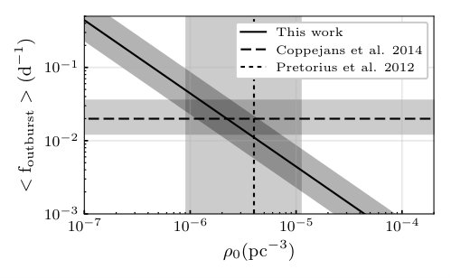 Figure 1
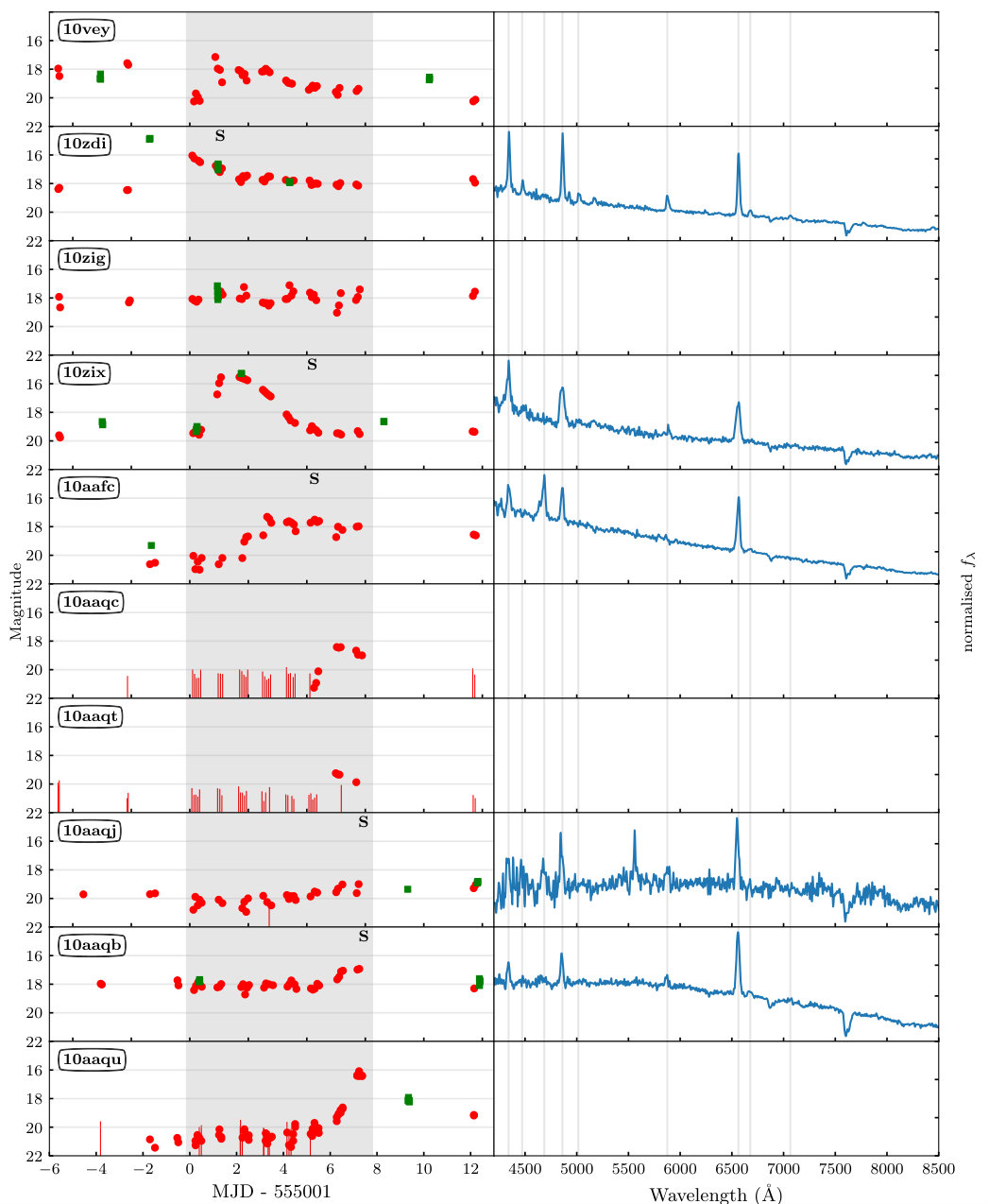 Figure 2
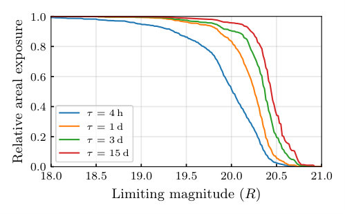 Figure 3
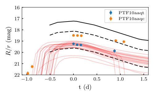 Figure 4
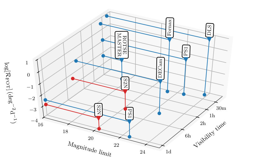 Figure 5
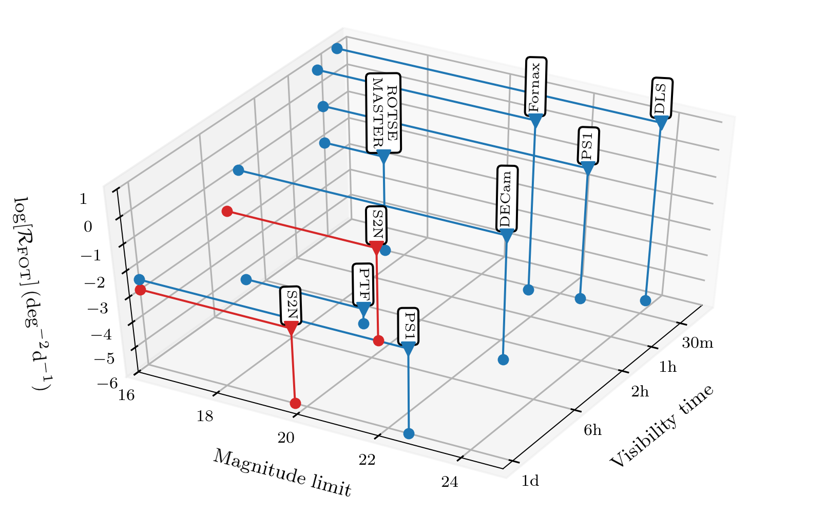 Figure 6
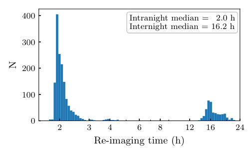 Figure 7
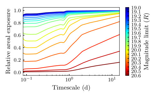 Figure 8
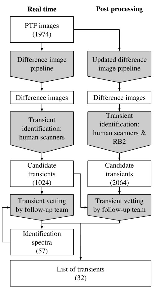 Figure 9
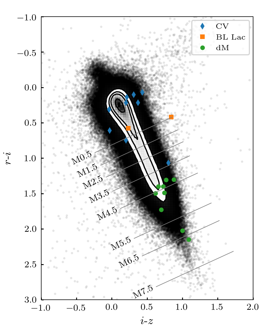 Figure 10
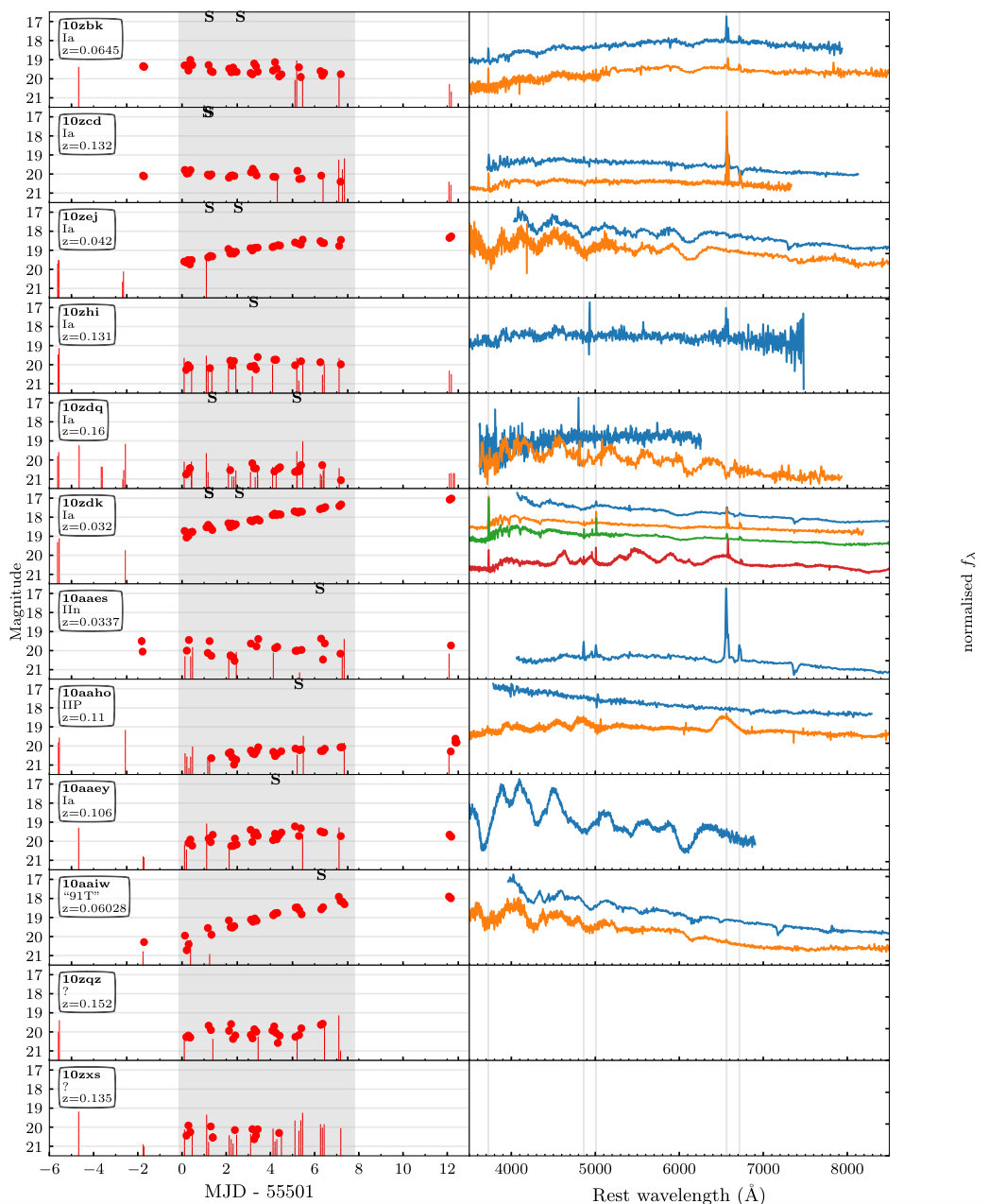 Figure 11
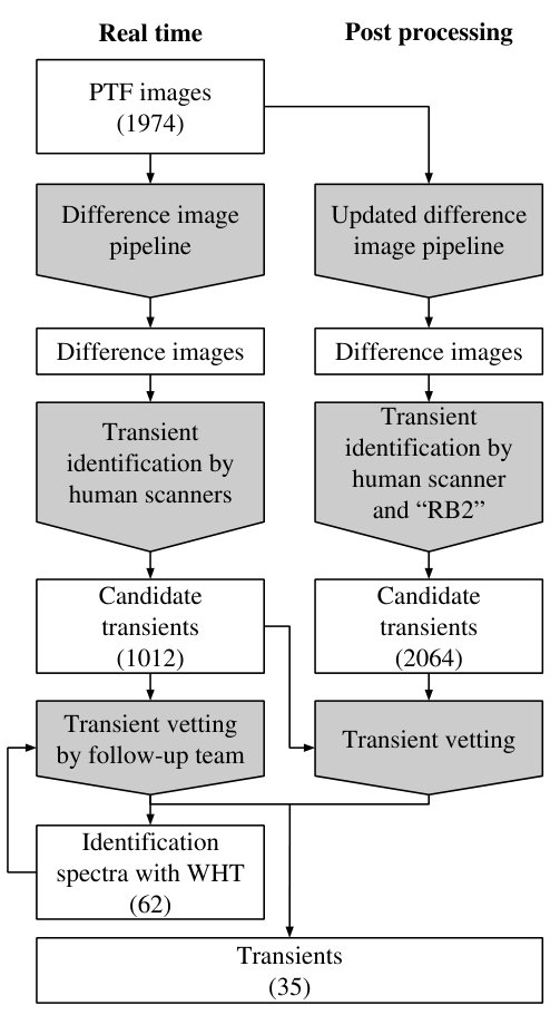 Figure 12
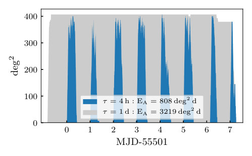 Figure 13
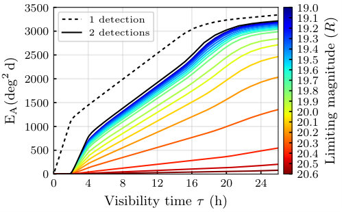 Figure 14
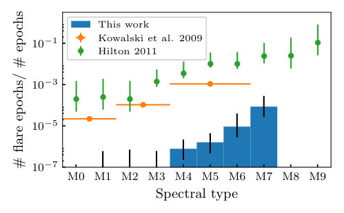 Figure 15
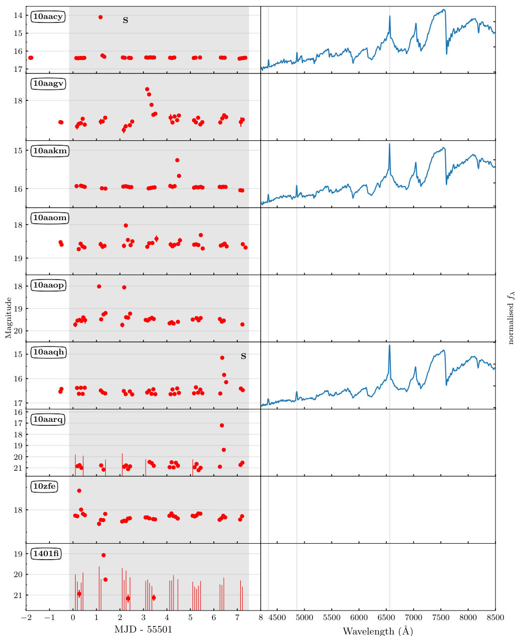 Figure 16
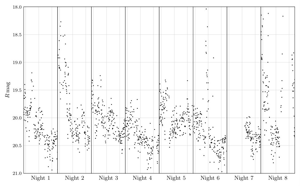 Figure 17
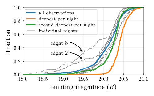 Figure 18
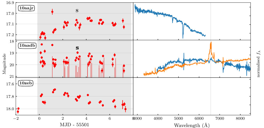 Figure 19
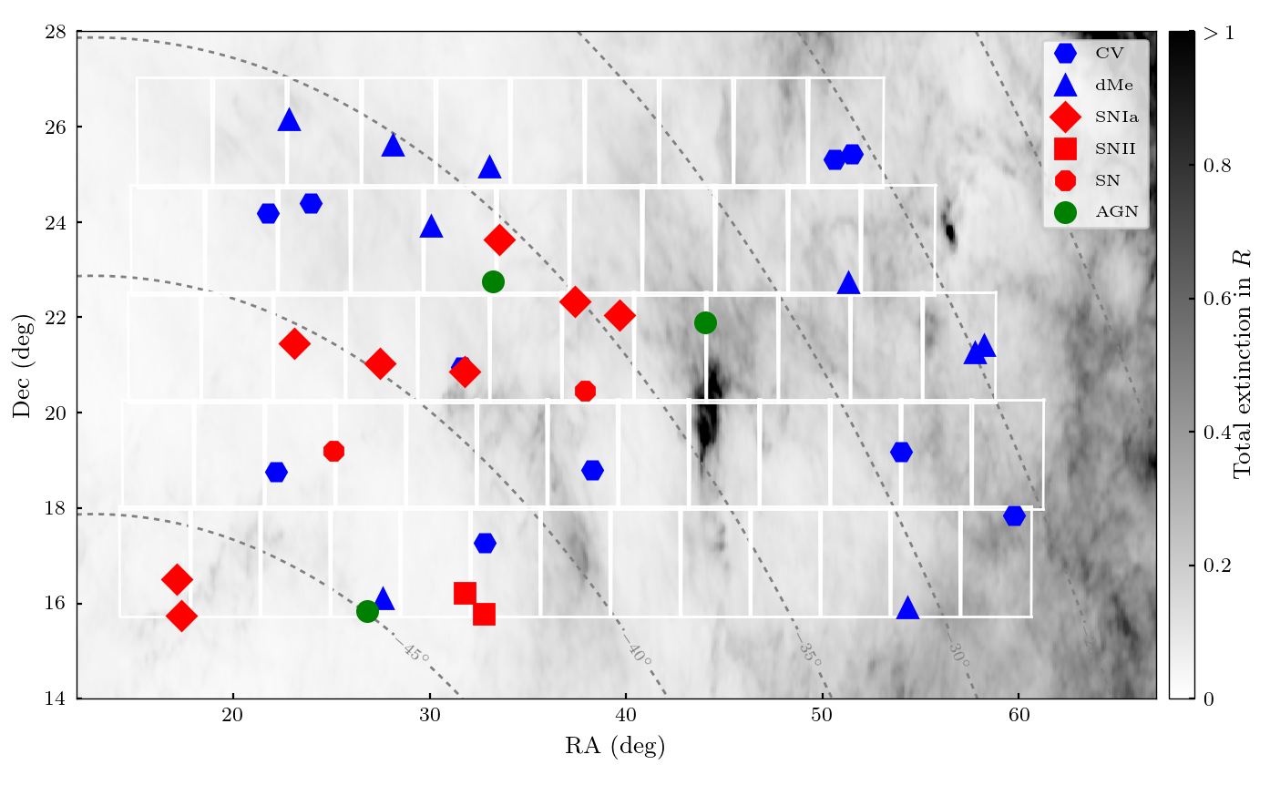 Figure 20
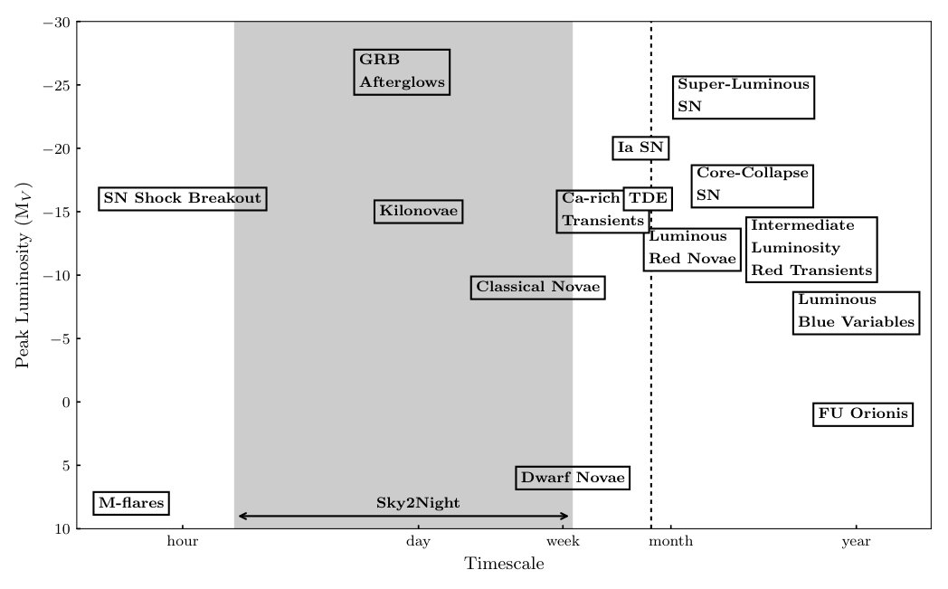 Figure 21
| Type | # |
|---|---|
| Point-source counterpart | |
| - Star | 873 |
| - QSO | 15 |
| - Faint star () | 3 |
| Galaxy counterpart | |
| - Nuclear | 48 |
| - Near galaxy | 12 |
| Artefact | 26 |
| Moving object | 35 |
| Total | 1012 |
| Name | Ra | Dec | First detection | Discovery | Type | counterpart | spectrum |
|---|---|---|---|---|---|---|---|
| PTF … | (°) | (°) | (MJD-55501) | (MJD-55501) | |||
| 10vey | 21.734133 | 24.188559 | -46.5 | -46.5 | CV | =19.37 | |
| 10aaqh | 58.242271 | 21.424262 | -3.76 | -1.78 | M-flare | =16.50 | ACAM |
| 10zbka | 37.393757 | 22.333575 | -1.76 | -1.72 | SN/Ia | galaxy | R.C. Spec, Kast |
| 10zcdb | 17.137369 | 16.502957 | -1.76 | 0.13 | SN/Ia | galaxy | ACAM, R.C. Spec |
| 10zejc,d | 31.760443 | 20.853715 | 0.1 | 0.19 | SN/Ia-“91bg”? | galaxy | ACAM |
| 10zebe | 26.82027 | 15.82885 | -1.82 | 0.22 | QSO/BL Lac | =19.20 | |
| 10zhib | 23.101224 | 21.455835 | 0.19 | 0.27 | SN/Ia | galaxy | R.C. Spec |
| 10zfe | 30.067678 | 23.926279 | 0.34 | 0.34 | M-flare | =18.15 | |
| 10zdq | 27.478711 | 21.033048 | 0.19 | 0.36 | SN/Ia | galaxy | ACAM |
| 10zdif | 31.639451 | 20.952067 | 0.1 | 0.44 | CV | =18.44 | ACAM |
| 10zdkg | 33.530525 | 23.630602 | 0.12 | 0.46 | SN/Ia | galaxy | ACAM, R.C. Spec, Kast, LRIS |
| 10zqz | 25.085293 | 19.205094 | 0.60 | 0.86 | SN | galaxy | |
| 10aacy | 27.623838 | 16.107371 | 1.17 | 1.17 | M-flare | =16.37 | ACAM |
| 10aadbh | 35.64689 | 25.137566 | -5.6 | 1.20 | AGN | galaxy | ACAM, DBSP |
| 10zigi | 22.159879 | 18.760014 | 1.31 | 1.31 | CV | =18.22 | |
| 10zixj | 32.792509 | 17.273396 | 1.16 | 1.33 | CV | =19.61 | ACAM |
| 10zxs | 37.87864 | 20.461258 | 0.20 | 1.89 | SN | galaxy | |
| 10aaop | 33.024992 | 25.166939 | 1.1 | 2.18 | M-flare | =19.51 | |
| 10aaesk | 31.791567 | 16.211025 | -19.81 | 2.20 | SN/IIn | galaxy | ACAM |
| 10aaom | 54.314202 | 15.914879 | 2.24 | 2.25 | M-flare | =18.58 | |
| 10aaho | 32.755376 | 15.785523 | 0.14 | 2.27 | SN/IIP | galaxy | ACAM, LRIS |
| 10aaey | 39.654895 | 22.056594 | 0.29 | 2.31 | SN/Ia | galaxy | LRIS |
| 10aafcl | 51.512414 | 25.425869 | 2.33 | 2.40 | CV | =20.17 | ACAM |
| 10aagv | 57.774944 | 21.256824 | 3.34 | 3.34 | M-flare | =18.34 | |
| 10aajrm | 33.219913 | 22.748068 | 0.26 | 4.10 | QSO/BL lac | =17.83 | |
| 10aaiwa | 17.338134 | 15.735881 | -2.71 | 4.13 | SN/Ia-“99T” | galaxy | ACAM, KAST |
| 10aakm | 51.319163 | 22.735708 | 0.14 | 4.51 | M-flare | =15.89 | ACAM |
| 10aaqci | 38.260974 | 18.806173 | 6.28 | 6.28 | CV | =22.03 | ACAM |
| 10aarq | 28.098845 | 25.613108 | 6.34 | 6.34 | M-flare | =20.68 | |
| 10aaqti | 23.952331 | 24.400854 | 6.24 | 6.40 | CV | =23.02 | |
| 10aaqj | 50.600737 | 25.309258 | 5.33 | 6.42 | CV | =20.16 | ACAM |
| 10aaqbi | 59.774695 | 17.842959 | 6.38 | 6.46 | CV | =18.00 | ACAM |
| 10aaqui | 53.982354 | 19.188484 | 6.36 | 6.52 | CV | =20.34 | |
| 1401fi | 22.82068 | 26.1559 | 1.29 | >8 | M-flare | =21.37 |
| Type | ( deg-2 d-1) | |
|---|---|---|
| Supernova - Ia | 8 | |
| Supernova - CC | 1 | |
| CV - DN | 5 | |
| CV - DN - mag | 2 | |
| M-flares | 9 | |
| M-flares - mag | 2 | |
| BL Lac flares | 2 | |
| FOTs (4 h) | 0 | |
| FOTs (1 d) | 0 |
| FieldID | RA (°) | Dec (°) | Ec. Lon. (°) | Ec. Lat. (°) | Gal. Lon. (°) | Gal. Lat. (°) | Brightest star (mag) | |
|---|---|---|---|---|---|---|---|---|
| 3430 | 16.0396 | 16.875 | 21.2721 | 9.2741 | 127.306 | -45.8887 | 0.045 | 5.68 |
| 3431 | 19.604 | 16.875 | 24.459 | 7.9678 | 132.161 | -45.5128 | 0.078 | 3.71 |
| 3432 | 23.1683 | 16.875 | 27.6492 | 6.6942 | 136.916 | -44.8742 | 0.089 | 3.71 |
| 3433 | 26.7327 | 16.875 | 30.8459 | 5.4573 | 141.528 | -43.9839 | 0.053 | 5.21 |
| 3434 | 30.297 | 16.875 | 34.0516 | 4.261 | 145.96 | -42.8563 | 0.061 | 5.21 |
| 3435 | 33.8614 | 16.875 | 37.2688 | 3.1092 | 150.189 | -41.5079 | 0.098 | 5.89 |
| 3436 | 37.4257 | 16.875 | 40.4995 | 2.0057 | 154.198 | -39.9567 | 0.454 | 6.05 |
| 3437 | 40.9901 | 16.875 | 43.7453 | 0.9542 | 157.982 | -38.2211 | 0.1 | 5.32 |
| 3438 | 44.5545 | 16.875 | 47.0077 | -0.0417 | 161.541 | -36.319 | 0.224 | 5.32 |
| 3439 | 48.1188 | 16.875 | 50.2875 | -0.9783 | 164.88 | -34.2677 | 0.129 | 6.1 |
| 3440 | 51.6832 | 16.875 | 53.5855 | -1.8524 | 168.01 | -32.0832 | 0.123 | 6.26 |
| 3441 | 55.2475 | 16.875 | 56.9018 | -2.6606 | 170.943 | -29.78 | 0.221 | 6 |
| 3442 | 58.8119 | 16.875 | 60.2362 | -3.3998 | 173.694 | -27.3716 | 0.436 | 5.91 |
| 3531 | 16.2 | 19.125 | 22.3031 | 11.2882 | 127.294 | -43.6335 | 0.04 | 4.77 |
| 3532 | 19.8 | 19.125 | 25.4973 | 9.9791 | 131.952 | -43.26 | 0.054 | 4.77 |
| 3533 | 23.4 | 19.125 | 28.6931 | 8.7045 | 136.519 | -42.6317 | 0.055 | 5.34 |
| 3534 | 27.0 | 19.125 | 31.8936 | 7.4682 | 140.956 | -41.7586 | 0.059 | 5.21 |
| 3535 | 30.6 | 19.125 | 35.1015 | 6.2741 | 145.233 | -40.6537 | 0.08 | 5.21 |
| 3536 | 34.2 | 19.125 | 38.3192 | 5.1263 | 149.324 | -39.3323 | 0.136 | 5.28 |
| 3537 | 37.8 | 19.125 | 41.5487 | 4.0284 | 153.216 | -37.8109 | 0.096 | 5.57 |
| 3538 | 41.4 | 19.125 | 44.7918 | 2.9841 | 156.9 | -36.1066 | 0.085 | 5.17 |
| 3539 | 45.0 | 19.125 | 48.0498 | 1.9971 | 160.376 | -34.2362 | 0.194 | 4.45 |
| 3540 | 48.6 | 19.125 | 51.3236 | 1.0707 | 163.647 | -32.216 | 0.106 | 4.45 |
| 3541 | 52.2 | 19.125 | 54.614 | 0.2084 | 166.722 | -30.0612 | 0.169 | 4.87 |
| 3542 | 55.8 | 19.125 | 57.921 | -0.5867 | 169.611 | -27.7861 | 0.405 | 5.67 |
| 3543 | 59.4 | 19.125 | 61.2446 | -1.3117 | 172.326 | -25.4034 | 0.321 | 5.62 |
| 3631 | 16.5306 | 21.375 | 23.4947 | 13.2383 | 127.489 | -41.3668 | 0.041 | 4.5 |
| 3632 | 20.2041 | 21.375 | 26.7269 | 11.9154 | 132.004 | -40.9786 | 0.048 | 4.77 |
| 3633 | 23.8775 | 21.375 | 29.9592 | 10.6295 | 136.434 | -40.3384 | 0.07 | 5.34 |
| 3634 | 27.551 | 21.375 | 33.1947 | 9.3848 | 140.743 | -39.4557 | 0.07 | 4.8 |
| 3635 | 31.2245 | 21.375 | 36.4363 | 8.1853 | 144.9 | -38.3429 | 0.126 | 4.8 |
| 3636 | 34.898 | 21.375 | 39.6865 | 7.0349 | 148.883 | -37.0148 | 0.101 | 5.04 |
| 3637 | 38.5714 | 21.375 | 42.9474 | 5.9376 | 152.679 | -35.487 | 0.135 | 5.47 |
| 3638 | 42.2449 | 21.375 | 46.2206 | 4.897 | 156.279 | -33.776 | 0.342 | 5.17 |
| 3639 | 45.9184 | 21.375 | 49.5076 | 3.9168 | 159.683 | -31.898 | 0.432 | 4.45 |
| 3640 | 49.5918 | 21.375 | 52.8094 | 3.0004 | 162.892 | -29.8688 | 0.333 | 4.45 |
| 3641 | 53.2653 | 21.375 | 56.1264 | 2.1513 | 165.913 | -27.7033 | 0.185 | 5.22 |
| 3642 | 56.9388 | 21.375 | 59.4589 | 1.3726 | 168.757 | -25.4154 | 0.191 | 5.43 |
| 3729 | 16.701 | 23.625 | 24.5571 | 15.2451 | 127.469 | -39.1113 | 0.043 | 4.5 |
| 3730 | 20.4124 | 23.625 | 27.7929 | 13.9204 | 131.812 | -38.7253 | 0.065 | 4.79 |
| 3731 | 24.1237 | 23.625 | 31.0272 | 12.6345 | 136.076 | -38.0941 | 0.1 | 6.24 |
| 3732 | 27.835 | 23.625 | 34.263 | 11.3916 | 140.229 | -37.2265 | 0.119 | 4.8 |
| 3733 | 31.5464 | 23.625 | 37.5033 | 10.1956 | 144.245 | -36.1341 | 0.084 | 4.8 |
| 3734 | 35.2577 | 23.625 | 40.7507 | 9.0505 | 148.101 | -34.8302 | 0.09 | 5.04 |
| 3735 | 38.9691 | 23.625 | 44.0071 | 7.9601 | 151.786 | -33.3295 | 0.134 | 5.47 |
| 3736 | 42.6804 | 23.625 | 47.2745 | 6.9281 | 155.289 | -31.6474 | 0.207 | 5.17 |
| 3737 | 46.3918 | 23.625 | 50.5542 | 5.958 | 158.61 | -29.799 | 0.141 | 5.17 |
| 3738 | 50.1031 | 23.625 | 53.847 | 5.0533 | 161.748 | -27.7994 | 0.212 | 5.46 |
| 3739 | 53.8144 | 23.625 | 57.1536 | 4.2172 | 164.71 | -25.6627 | 0.22 | 3.6 |
| 3826 | 17.0526 | 25.875 | 25.7913 | 17.1841 | 127.647 | -36.8431 | 0.086 | 4.75 |
| 3827 | 20.8421 | 25.875 | 29.0625 | 15.8464 | 131.867 | -36.4421 | 0.119 | 4.75 |
| 3828 | 24.6316 | 25.875 | 32.3304 | 14.5504 | 136.012 | -35.7978 | 0.1 | 6.25 |
| 3829 | 28.4211 | 25.875 | 35.5986 | 13.3004 | 140.052 | -34.9189 | 0.116 | 4.8 |
| 3830 | 32.2105 | 25.875 | 38.87 | 12.1004 | 143.961 | -33.8163 | 0.063 | 4.8 |
| 3831 | 36.0 | 25.875 | 42.1473 | 10.9545 | 147.72 | -32.503 | 0.088 | 5.02 |
| 3832 | 39.7895 | 25.875 | 45.4327 | 9.8665 | 151.315 | -30.9931 | 0.153 | 3.58 |
| 3833 | 43.5789 | 25.875 | 48.7279 | 8.8402 | 154.739 | -29.3015 | 0.096 | 3.58 |
| 3834 | 47.3684 | 25.875 | 52.0342 | 7.8791 | 157.988 | -27.443 | 0.197 | 5.46 |
| 3835 | 51.1579 | 25.875 | 55.3527 | 6.9866 | 161.063 | -25.432 | 0.152 | 5.64 |
| Night 1 | Night 2 | Night 3 | Night 4 | Night 5 | Night 6 | Night 7 | Night 8 | ||
|---|---|---|---|---|---|---|---|---|---|
| PTF | time lost (h) | 0.6 | 3.7 | 0.1 | 0.2 | 0.7 | 0.4 | 3.7 | 6.0 |
| seeing (″) | 2.5-3.5 | 3.0 | 3.0 | 2.5 | 2.0-3.5 | 2.0 | 3.0 | 2.5-3.5 | |
| cloud conditions | good | good | good | ok | ok | ok | bad/ok | bad | |
| WHT | time lost (h) | 0 | 3.0 | 10.3 | 0 | 0 | 0 | 6.7 | |
| seeing (″) | 1.5-2.5 | 1.5-3.0 | 2.5 | 2.5 | 1.5-2.5 | 1.0 | 2-3 | ||
| cloud conditions | good | ok-bad | bad | good | good | good | good |
| FieldID | Night 1 | Night 2 | Night 3 | Night 4 | Night 5 | Night 6 | Night 7 | Night 8 | Total |
|---|---|---|---|---|---|---|---|---|---|
| 3430 | 4 | 3 | 4 | 4 | 3 | 4 | 2 | 4 | 28 |
| 3431 | 4 | 3 | 5 | 5 | 3 | 4 | 2 | 4 | 30 |
| 3432 | 4 | 3 | 5 | 5 | 3 | 4 | 3 | 4 | 31 |
| 3433 | 5 | 3 | 4 | 5 | 3 | 3 | 3 | 4 | 30 |
| 3434 | 5 | 3 | 5 | 5 | 3 | 4 | 3 | 4 | 32 |
| 3435 | 5 | 3 | 5 | 5 | 4 | 5 | 3 | 4 | 34 |
| 3436 | 5 | 4 | 5 | 5 | 3 | 4 | 3 | 3 | 32 |
| 3437 | 5 | 3 | 5 | 4 | 3 | 5 | 3 | 3 | 31 |
| 3438 | 5 | 3 | 4 | 5 | 3 | 5 | 3 | 3 | 31 |
| 3439 | 5 | 3 | 5 | 5 | 4 | 5 | 3 | 3 | 33 |
| 3440 | 5 | 3 | 5 | 5 | 4 | 5 | 4 | 3 | 34 |
| 3441 | 4 | 3 | 5 | 5 | 5 | 5 | 4 | 3 | 34 |
| 3442 | 5 | 3 | 5 | 4 | 5 | 5 | 4 | 3 | 34 |
| 3531 | 5 | 5 | 4 | 5 | 5 | 4 | 2 | 3 | 33 |
| 3532 | 5 | 2 | 4 | 5 | 5 | 4 | 3 | 3 | 31 |
| 3533 | 4 | 3 | 4 | 5 | 5 | 4 | 3 | 3 | 31 |
| 3534 | 5 | 4 | 4 | 5 | 5 | 4 | 3 | 3 | 33 |
| 3535 | 5 | 4 | 5 | 5 | 5 | 5 | 3 | 4 | 36 |
| 3536 | 4 | 4 | 4 | 5 | 5 | 5 | 3 | 4 | 34 |
| 3537 | 5 | 4 | 5 | 5 | 5 | 5 | 3 | 4 | 36 |
| 3538 | 4 | 4 | 5 | 6 | 6 | 5 | 3 | 3 | 36 |
| 3539 | 5 | 3 | 5 | 5 | 4 | 5 | 4 | 3 | 34 |
| 3540 | 5 | 3 | 5 | 5 | 5 | 5 | 4 | 3 | 35 |
| 3541 | 5 | 3 | 5 | 5 | 5 | 5 | 4 | 3 | 35 |
| 3542 | 4 | 3 | 5 | 5 | 5 | 6 | 4 | 3 | 35 |
| 3543 | 4 | 3 | 5 | 5 | 5 | 5 | 4 | 2 | 33 |
| 3631 | 5 | 3 | 5 | 5 | 4 | 4 | 2 | 2 | 30 |
| 3632 | 5 | 4 | 5 | 5 | 4 | 4 | 3 | 3 | 33 |
| 3633 | 5 | 4 | 5 | 5 | 3 | 5 | 3 | 2 | 32 |
| 3634 | 5 | 2 | 5 | 5 | 5 | 5 | 3 | 2 | 32 |
| 3635 | 5 | 4 | 5 | 5 | 4 | 5 | 3 | 2 | 33 |
| 3636 | 6 | 3 | 5 | 6 | 5 | 5 | 3 | 1 | 34 |
| 3637 | 5 | 4 | 5 | 5 | 5 | 5 | 3 | 3 | 35 |
| 3638 | 5 | 2 | 5 | 6 | 5 | 5 | 4 | 3 | 35 |
| 3639 | 5 | 3 | 5 | 5 | 5 | 4 | 4 | 2 | 33 |
| 3640 | 5 | 3 | 5 | 5 | 5 | 5 | 4 | 2 | 34 |
| 3641 | 5 | 3 | 5 | 4 | 5 | 5 | 4 | 2 | 33 |
| 3642 | 5 | 3 | 5 | 5 | 5 | 5 | 4 | 2 | 34 |
| 3729 | 5 | 3 | 5 | 5 | 5 | 4 | 3 | 2 | 32 |
| 3730 | 4 | 4 | 5 | 5 | 4 | 5 | 3 | 2 | 32 |
| 3731 | 5 | 4 | 5 | 4 | 5 | 5 | 4 | 1 | 33 |
| 3732 | 6 | 4 | 5 | 5 | 4 | 5 | 4 | 2 | 35 |
| 3733 | 6 | 4 | 5 | 5 | 5 | 5 | 4 | 2 | 36 |
| 3734 | 5 | 4 | 5 | 6 | 5 | 5 | 4 | 2 | 36 |
| 3735 | 5 | 4 | 6 | 6 | 5 | 5 | 4 | 1 | 36 |
| 3736 | 5 | 4 | 5 | 5 | 5 | 6 | 4 | 2 | 36 |
| 3737 | 5 | 3 | 5 | 5 | 5 | 5 | 4 | 2 | 34 |
| 3738 | 5 | 3 | 5 | 5 | 5 | 5 | 4 | 2 | 34 |
| 3739 | 5 | 3 | 5 | 5 | 5 | 5 | 4 | 2 | 34 |
| 3826 | 5 | 4 | 5 | 5 | 4 | 5 | 3 | 2 | 33 |
| 3827 | 5 | 4 | 5 | 4 | 5 | 5 | 3 | 2 | 33 |
| 3828 | 5 | 4 | 5 | 5 | 4 | 5 | 3 | 2 | 33 |
| 3829 | 6 | 4 | 5 | 5 | 5 | 5 | 3 | 2 | 35 |
| 3830 | 6 | 4 | 5 | 5 | 4 | 5 | 3 | 1 | 33 |
| 3831 | 5 | 4 | 6 | 6 | 5 | 6 | 3 | 2 | 37 |
| 3832 | 5 | 4 | 4 | 6 | 5 | 6 | 4 | 2 | 36 |
| 3833 | 5 | 3 | 5 | 5 | 5 | 6 | 4 | 2 | 35 |
| 3834 | 5 | 3 | 4 | 5 | 5 | 5 | 4 | 2 | 33 |
| 3835 | 5 | 3 | 5 | 5 | 5 | 5 | 4 | 2 | 34 |
| median | 5 | 3 | 5 | 5 | 5 | 5 | 3 | 2 | 34 |
| total | 290 | 200 | 287 | 296 | 266 | 285 | 199 | 151 | 1974 |
| Name | Type | Redshift | peaktime |
|---|---|---|---|
| PTF … | (z) | (MJD-55501) | |
| 10zbk | Ia | ||
| 10zcd | Ia | ||
| 10zej | Ia “91bg”: | ||
| 10zhi | Ia | ||
| 10zdq | Ia | ||
| 10zdk | Ia | ||
| 10aaes | IIn | ||
| 10aaho | IIP | ||
| 10aaey | Ia | ||
| 10aaiw | Ia “99T” | ||
| 10zxs | ? | ||
| 10zqz | ? |
| Name | type | quiescence | |
|---|---|---|---|
| PTF … | (mag) | (mag) | |
| 10vey | U Gem | 3.4 | |
| 10zdi | U Gem | 2.4 | |
| 10zig | SU UMa:/WZ Sge: | 5.5 | |
| 10zix | U Gem | 3.9 | |
| 10aafc | U Gem | 2.5 | |
| 10aaqc | U Gem | 3.5 | |
| 10aaqt | U Gem | 4.5 | |
| 10aaqj | AM Her: | 1.0 | |
| 10aaqb | U Gem | 1.2 | |
| 10aaqu | U Gem | 4.3 |
| Name | Sp type | quiescence | time scale | ||
|---|---|---|---|---|---|
| PTF … | (mag) | (mag) | (h) | ||
| 10aacy | M4 | 16.4 | 2.3 | 0.5(1) | 32.0 |
| 10aagv | M5 | 18.3 | 0.6 | 4.6(4) | 32.0 |
| 10aakm | M4 | 15.9 | 0.6 | 1.6(1) | 32.0 |
| 10aaom | M5 | 18.7 | 0.7 | 1.3(2) | 31.4 |
| 10aaop | M7 | 19.5 | 1.5/1.5 | <0.3/<0.6 | 30.0/30.4 |
| 10aaqh | M5 | 16.5 | 1.3 | 1.9(1) | 32.1 |
| 10aarq | M6 | 20.7 | 3.5 | 0.8(1) | 31.6 |
| 10zfe | M4 | 18.2 | 0.6 | 1.4(1) | 32.0 |
| 1401fi | M4 | 21.3 | 2.2 | 1.2(2) | 34.0 |
Peer Reviews
No public reviews on file for this paper yet. If you reviewed it on a platform where reviews are public (OpenReview, ICLR, NeurIPS, ICML), you can paste yours below so the community can read it here.
Videos
No videos yet. Explain this paper in a talk, walkthrough, or lecture? Add one.
The Palomar Transient Factory Sky2Night programme
J. van Roestel1, P.J. Groot1, T. Kupfer2,3,4, K. Verbeek1, S. van Velzen5, M. Bours6, P. Nugent7, T. Prince4, D. Levitan 4, S. Nissanke1, S.R. Kulkarni4, R.R. Laher8
1 Department of Astrophysics/IMAPP, Radboud University Nijmegen, P.O.Box 9010, 6500 GL, Nijmegen, The Netherlands
2 Kavli Institute for Theoretical Physics, University of California, Santa Barbara, CA 93106, USA
3 Department of Physics, University of California, Santa Barbara, CA 93106, USA
4 Cahill Center for Astronomy and Astrophysics, California Institute of Technology, Pasadena, CA 91125
5 Center of Cosmology and Particle Physics, New York University, New York, NY 10003, USA
6 Instituto de Física y Astronomía, Universidad de Valparaíso, Avenida Gran Bretana 1111, Valparaíso 2360102, Chile
7 Lawrence Berkeley National Laboratory, UC Berkley Department of Astronomy, Berkeley, CA, USA
8 Spitzer Science Center, California Institute of Technology, Pasadena, CA 91125, USA [email protected]
(Accepted XXX. Received YYY; in original form ZZZ)
Abstract
We present results of the Sky2Night project: a systematic, unbiased search for fast optical transients with the Palomar Transient Factory. We have observed 407 deg2 in -band for 8 nights at a cadence of 2 hours. During the entire duration of the project, the 4.2 m William Herschel Telescope on La Palma was dedicated to obtaining identification spectra for the detected transients. During the search, we found 12 supernovae, 10 outbursting cataclysmic variables, 9 flaring M-stars, 3 flaring active Galactic nuclei and no extragalactic fast optical transients. Using this systematic survey for transients, we have calculated robust observed rates for the detected types of transients, and upper limits of the rate of extragalactic fast optical transients of deg*-2* d*-1* and deg*-2* d*-1* for timescales of 4 h and 1 d and a limiting magnitude of . We use the results of this project to determine what kind of and how many astrophysical false positives we can expect when following up gravitational wave detections in search for kilonovae.
keywords:
supernovae: general – stars: dwarf novae
††pubyear: 2018††pagerange: The Palomar Transient Factory Sky2Night programme–A
1 Introduction
Fast optical transients are transients which appear and disappear within 24 hours or less. The rate of fast optical transients is not well known (see Fig. 1). The reason why the fast transient sky has not yet been systematically explored is due to technical limitations. To find fast transients a high cadence is required, which means that area and/or depth need to be sacrificed. For example, a 3-day cadence supernova survey can cover an area 100 times larger than a survey of optical transients with a cadence of 1 hour (using the same setup). In addition, follow up of fast optical transients is difficult since it requires rapid detection and identification of the transient and triggering of a follow-up telescope.
For this reason, almost all known extragalactic fast optical transients (timescales of less than 1 day) have been found as a counterpart of a transient detected at another wavelength where larger solid angle facilities are possible, e.g. X-ray or gamma-ray satellites. The most well studied are gamma-ray burst afterglows: interactions between highly relativistic outflows (jets) and their environment (e.g. Piran, 1999). Although they can be bright, because of the low rate ( with , Cenko et al., 2015) and in particular because of their rapid fading ( magnitudes per hour, e.g. Singer et al., 2015; Fong et al., 2015) they are very difficult to find in blind searches. So far, only one111a strong candidate without a gamma-ray detection is described by Cenko et al. (2013) GRB afterglow has been found in a blind search: iPTF14yb (Cenko et al., 2015).
In searches for fast extragalactic transients, many Galactic fast optical transients are detected: outbursts of stars in our Galaxy with short ( d) timescales. These are sometimes considered a ‘foreground fog’, but they are also interesting to study in their own right. Flaring M-dwarfs are the most common Galactic fast optical transients with typical time scales of 10-100 minutes (Hawley et al., 2014; Silverberg et al., 2016) up to 7 hours (Kowalski et al., 2010) and outburst magnitudes up to 9 magnitudes in V-band (e.g. Schmidt et al., 2014). Understanding M-flare rates and intensities have recently become important with regards to planetary habitability (e.g. Vida et al., 2017). The other type of common Galactic transients are eruptions in compact binary systems with an accretion disk. The most common are dwarf novae (DN), caused by accretion disc instabilities in systems where a white dwarf accretes mass from a main sequence companion. These outbursts can brighten the system by up to 8 magnitudes (e.g. WZ Sge, Harrison et al., 2004), with short rise timescales ( 1 day) and can last for a few days to weeks (Warner, 2003).
In 2017, the aLIGO/aVirgo gravitational wave observatories (LIGO Scientific Collaboration et al., 2015; Acernese et al., 2015) detected the first binary neutron star (BNS) merger (Abbott et al., 2017a). Rapid optical follow up of this event resulted in the discovery of the optical counterpart AT 2017gfo (Abbott et al. 2017b, c, see also: Andreoni et al. 2017; Arcavi et al. 2017; Coulter et al. 2017; Cowperthwaite et al. 2017b; Díaz et al. 2017; Drout et al. 2017; Evans et al. 2017; Hu et al. 2017; Kasliwal et al. 2017; Lipunov et al. 2018; Pian et al. 2017; Pozanenko et al. 2018; Shappee et al. 2017; Smartt et al. 2017; Tanvir et al. 2017; Troja et al. 2017; Utsumi et al. 2017; Valenti et al. 2017). The optical counterpart, called a kilonova, had been theorized to accompany a BNS merger by Li & Paczyński (1998); Kulkarni (2005); Metzger et al. (2010); Roberts et al. (2011); Barnes & Kasen (2013); Tanaka & Hotokezaka (2013); Metzger & Fernández (2014); Kasen et al. (2015). AT 2017gfo is consistent with the kilonova model predictions: it was fading rapidly (), had a peak absolute magnitude of mag and displayed rapid reddening ( in ).
The optical signal can be well modelled using either two or three outflow components. The two-component models are a combination of a rapidly fading ‘blue’ component, emitted by fast-moving, low opacity material, and a slower fading ‘red’ component emitted by slower-moving, high opacity material. Three component models add an addition ‘purple’ component, with intermediate velocity and opacity. Villar et al. (2017) show that a three-component model is the best explanation for kilonova AT 2017gfo. However, we should be aware that future kilonovae can be quite different than AT 2017gfo. For example, a lower amount of ejected mass and a different viewing angle results in a kilonovae which is significantly fainter, from down to (e.g. Kasen et al., 2015; Rosswog et al., 2017).
Currently, the aLIGO/aVirgo detectors are being upgraded, increasing the distance (and thus volume) at which they can detect BNS mergers. However, the localisation of the events will remain relatively poor (120-180 deg2, depending on the SNR of the event, Abbott et al., 2016). This means after the detection of a BNS merger, optical telescopes will still have to search a large area to find the faint optical counterpart, mag at 200 Mpc if it is similar to AT 2017gfo. One of the problems is that in such a large area and magnitude limit, many other (fast) transients will appear which can be confused for a kilonova; a ‘needle-in-the-haystack’ problem.
In the last decade, there have been a few studies that performed a blind search for fast transients in an attempt to determine the observed rate of fast optical transients. One of the earliest attempts was by Becker et al. (2004). They carried out an unbiased transients search on the data from the Deep Lensing Survey (DLS, Wittman et al., 2002) and found two M-flares and one potential extragalactic transient (OT20030305). However, follow up of the quiescent counterpart by Kulkarni & Rau (2006) shows that OT20030305 is also a flaring M-star. Other searches also found only Galactic transients, mainly cataclysmic variables (CVs) and M-dwarf flares. For example, Rykoff et al. (2005) used the ROTSE-II survey to search for untriggered GRBs but found only six outbursting cataclysmic variables. Rau et al. (2008) performed a high cadence survey on the Fornax galaxy cluster (cadence 32 min, depth B=22 mag). They also did not find any extragalactic fast optical transients in their search. The first multi-colour search for fast optical transients was performed by Berger et al. (2013), who showed that colours are very useful in identifying the transients. In their search for fast transients, they only found flares on faint M-stars and slow-moving asteroids. More recently, Cowperthwaite et al. (2017a) and Utsumi et al. (2018) performed multi-colour surveys with the goal to measure the rate of false positives when searching for kilonovae.
In this paper, we present an 8-day unbiased search for all transients in 407 deg2 of the sky. The search was combined with rapid, unbiased spectroscopic follow-up. To identify the transients we used the Palomar Transient Factory (PTF) and for immediate (within 24 hours) spectroscopic follow-up we used the William Herschel Telescope (WHT, Boksenberg, 1985). The main goals of the project are to measure the rate of intra-night transients (Galactic and extragalactic) and to determine the expected types of false positives when searching for the optical counterpart of gravitational waves by BNS mergers. The survey design is discussed in Section 2. The execution of the observations and data reduction are described in Section 3. The results: the survey characteristics, an overview of all detected transients, and the observed transient rates are presented in Section 4. We discuss the results in Section 5. The last section summarizes the paper and lists the main conclusions.
2 Survey design
The project consists of two parts: identification of transients with PTF, and rapid spectroscopic classification with the WHT.
To search the sky for transients, PTF used the 48-inch Oschin Schmidt Telescope at Palomar Observatory (P48), equipped with the CFH12K camera. The mosaic camera consists of 11 working CCDs with 4k2k pixels each. The system has a pixel scale of /pixel and a total field of view of 7.26 square degrees (Rau et al., 2009; Law et al., 2009). P48 was available for 8 nights of dark time on 2010 November 1–8 (in MJD range 55501.08–55508.85). We used the standard PTF setup of 60 s exposure times and the filter ( in the rest of the paper). We chose a target cadence of 2 hours and observed the same 59 PTF fields every night (see Table 4 for an overview). The fields are adjacent to each other on the sky and slightly overlapping, so the effective area covered is 407 deg2. The fields were selected such that they were observable the entire night and are located at an intermediate Galactic latitude (), allowing us to study both Galactic and extragalactic transients (see Fig. 1). The ecliptic latitude of the fields is between .
To be able to rapidly identify fast transients, PTF used an automated image processing pipeline which does bias and flatfield corrections, source extraction and image subtraction on all new images (Cao et al., 2016). Reference images of the target fields were obtained 14–16 days before the start of the project. Each reference image was constructed using at least 5 individual images. The difference images were presented to human scanners to identify transient candidates of interest and reject false positives. The best candidates were marked for follow-up spectroscopy.
We used the 4.2 m William Herschel Telescope (WHT) on La Palma, Spain, to obtain classification spectra of new transients. The WHT was dedicated for this purpose for 7 nights starting after the first night of PTF observations (MJD 55501.75). The instrument used to observe the transients was ACAM (Benn et al., 2008). ACAM is both an imager and low-resolution spectrograph (, 4000–9000 Å) and is therefore ideally suited for rapid transient identification. We first observed the candidate transients with ACAM in imaging mode to confirm if they are real and to determine the brightness, followed by an identification spectrum.
3 Observations
During the project, the weather at the P48 was mostly good. Fifteen per cent of the time was lost due to bad weather, mostly during nights 2, 7, and 8. The seeing was typically 2.5″, but it was highly variable and regularly increased up to 4″ (Table 5). A total of 1974 exposures were obtained, with a median of 5 exposures per field per night. Fewer observations were obtained during nights 2, 7, and 8; with a median of 3, 3, and 2 observations per field. A full overview of all PTF observations can be found in Table 6.
Fig. 2 shows a schematic overview of the data reduction and transient detection process. The new images were processed and difference images were created by the PTF pipeline as quickly as possible (see Sec. 2). This ranged from half an hour to a few hours after the observation because the image processing pipeline could not keep up with the flow of incoming images. As soon as the difference images were available they were analysed by multiple human scanners to identify new transients. Identifying the real transients on the difference images was not trivial since the difference images contained many artefacts (e.g. slight misalignments of the images, bad pixels). To reduce the time spend on visual inspection of candidates, we only inspected candidate transients which had two or more detections. This was done to get rid of asteroids but also filtered out some of the artefacts. In addition, the human scanners were assisted by a machine learning algorithm to get rid of the most obvious false positives (a rudimentary version of the ‘RealBogus’ pipeline, see Bloom et al. 2012, Cao et al. 2016 and also Smith et al. 2011). A total of 1012 candidate transients were judged by the human scanners to be potentially real, and these were passed on for further inspection by the follow-up team at the WHT.
The 1012 candidate transients were more carefully vetted by the follow-up team by inspecting the images obtained by PTF and, if available, SDSS images (Abazajian et al., 2009). In addition, we checked if the target corresponded to a known object in SIMBAD database222http://simbad.u-strasbg.fr/simbad/. An overview of the different kinds of transient candidates is given in Table 1. The bulk of the potential transients were associated with a known point-like source. The majority (873) of these were either due to bad subtraction of a star or low amplitude variability of a star. Besides variable stars, there were also 15 QSOs which brightened significantly during the project. We found three transient candidates without a counterpart in the PTF images, but for which a point-source was detected in the SDSS images. For all three, the SDSS and Pan-STARRS catalogues indicate that they are pointsources. A number of potential transients (60) were found near a galaxy. The majority of these (48) were at the core of the galaxy, and it is difficult to determine if this is a bad subtraction, AGN activity, or a supernova in the core of a galaxy. Five of these could be matched to a known AGN. Experience with other PTF data indicates that the remaining nuclear transients are likely bad subtractions or AGN. The 12 remaining transients with a nearby galaxy were strong supernova candidates. A few objects (35) were initially flagged as transients but were later identified as moving objects. In addition, 26 candidates were caused by artefacts (bad pixels, very bright stars and ‘ghosts’).
The PTF imaging data was thoroughly re-analysed in 2014 to make sure no transients were missed during the initial search (the right column in Fig. 2). The images were reprocessed using an improved version of the image processing pipeline. New difference images were made. All sources present on the new difference images were analysed using the ‘RealBogus2’ pipeline (Brink et al., 2013; Cao et al., 2016). We used a lower than normal threshold value of 0.3, compared to the 0.53 advised in the paper. This lower threshold corresponds to a missed detection rate of 5 per cent (compared to 10 per cent for a threshold of 0.53). This second search resulted in 2064 candidates transients, of which 105 overlap with the initial sample of 1012 sources. All these transient candidates were vetted using PTF, SDSS and Pan-STARRS (Chambers et al., 2016) images and CRTS light curves (Drake et al., 2009) and also using the SIMBAD database. This re-analysis recovered all real transients identified by the human scanners during the Sky2Night run. However, we also identified 2 faint supernovae and 5 flaring M-stars in the overlapping sample of transients. In addition, one new flaring M-star was found that was missed entirely during the initial search.
The most promising candidate transients found during the real-time search, typically transients candidates which were bright or were rapidly getting brighter, or were located off-centre from a galaxy, were observed with the WHT telescope. The results are shown in Table 7. The majority of the supernovae (8) are of type Ia. Since we obtained both a spectrum and an 8-day light curve, there is little uncertainty in the classification. The subtypes are more difficult to determine, but all except two, appear to be normal type Ia supernovae (for an overview of Ia subtypes, see for example Taubenberger, 2017). PTF10aaiw, for which we have two spectra, is a “91T”-like supernova (Filippenko et al., 1992b) according to the cross-correlation with template spectra. The spectra of PTF10aaiw show a shallow Si ii 6355 Å absorption line and deep Fe iii absorption features, which are the main features discriminating “91T”-type supernovae from normal SNIa supernovae. In addition, the absolute peak magnitude as determined from the light curve fit, , is consistent with being a “91T”-type supernova. PTF10zej could be a “91bg”-type supernova (Filippenko et al., 1992a); the obtained spectra match almost equally well with “91bg”-templates and normal Ia-template spectra. The estimated absolute magnitude is only , which puts it at the boundary between normal Ia supernova and “91bg”-type supernovae. With the available data, we cannot make a certain sub-classification of the subtype of PTF10zej. The results are shown in Table 7. The majority of the supernovae (8) are of type Ia. Since we obtained both a spectrum and an 8-day light curve, there is little uncertainty in the classification. The subtypes are more difficult to determine, but all except two, appear to be normal type Ia supernovae (for an overview of Ia subtypes, see for example Taubenberger, 2017). PTF10aaiw, for which we have two spectra, is a “91T”-like supernova (Filippenko et al., 1992b) according to the cross-correlation with template spectra. The spectra of PTF10aaiw show a shallow Si ii 6355 Å absorption line and deep Fe iii absorption features, which are the main features discriminating “91T”-type supernovae from normal SNIa supernovae. In addition, the absolute peak magnitude as determined from the light curve fit, , is consistent with being a “91T”-type supernova. PTF10zej could be a “91bg”-type supernova (Filippenko et al., 1992a); the obtained spectra match almost equally well with “91bg”-templates and normal Ia-template spectra. The estimated absolute magnitude is only , which puts it at the boundary between normal Ia supernova and “91bg”-type supernovae. With the available data, we cannot make a certain sub-classification of the subtype of PTF10zej. During the spectroscopic follow-up, the weather was variable. Most nights were clear, but during nights 2 and 3 time was lost due to passing clouds. Although night 7 was clear, about half the time was lost due to high humidity. The seeing during the nights varied between 0.8″and 4″. Table 5 shows an overview of the weather conditions at the WHT. A total of 62 transient candidates were observed. Exposure-times of the spectra range between 300 seconds and 1200 seconds. For calibration, either standard star SP2157+261 or SP0804+751 were observed at the beginning or end of the night. A quick reduction of the spectra was performed within 24 hours in order to identify any events which might need additional follow-up. The data were later reduced using standard procedures using iraf. For some transients, spectra were obtained with other telescopes as part of the PTF collaboration and were also used in the identification of transients (see also Table 2). All these spectra (including header information) are available on Wiserep333https://wiserep.weizmann.ac.il/ (Yaron & Gal-Yam, 2012).
4 Results
4.1 Survey characteristics
An overview of the most important metrics of the survey is given in Fig. 3. The time between observations, generally referred to as cadence, is given in the top left panel in Fig. 3. The median time between observations is 2.0 h within a night and almost all fields have been revisited within 3 hours. There is also a longer delay of about 16.8 h between revisits, which is due to the day-night cycle.
The limiting magnitude of the observations are shown in the top right panel. We empirically measure the limiting magnitude by calculating the \nth95 percentile magnitude of all sources detected in the image. The source detection by PTF is performed with Sextractor (Bertin & Arnouts, 1996) with a detection threshold of 4 standard deviations above the background noise. The median limiting magnitude of all observations is mag, with 95 per cent of the observations in the range of mag and mag (top right panel in Fig. 3). The figure also shows the distribution of the limiting magnitude of the deepest image per night (median mag) and the second deepest image per night (median mag), which is the relevant measure for transients which are visible for longer than 1 day. In addition, the distribution for individual nights is plotted, which shows that the nights are comparable, except for nights 2 and 8, due to clouds. Note that the limiting magnitudes are not randomly distributed in each night, but vary as a function of time in the night (see Fig. 10). This is caused by the airmass related extinction as the fields are tracked from horizon to horizon. At the beginning of the night, the limiting magnitude is about mag per exposure and increases to mag during the middle of the night, and then decreases again to mag toward the end of the night. A few spikes can be seen in the limiting magnitudes as a function of time which are caused by passing clouds.
In order to calculate an observed rate of transients, we need to determine how much area we have effectively monitored and for how long: the areal exposure (units: deg2 d), which is a function of how long a transient is visible (). To calculate the areal exposure for Sky2Night, we test if a transient (visible for a set duration ) would have been detected at least twice in our survey. The result for transients visible for =4 h and =1 d is shown as the shaded area in the mid-left panel in Fig. 3. The total areal exposure for a given visibility time can be calculated by integrating over time (i.e. the area of the shaded surface in the mid-left panel). The areal exposure as a function of visibility time () is shown in the mid-right panel. Here we also show the areal exposure if we take the limiting magnitude of the images into account. The bottom panel shows the same information in a different way: the fraction of areal exposure that is available as a function of magnitude. This shows that there is almost no loss of areal exposure for long timescale transient before magnitude , but for the short timescale transients, the areal exposure already starts to decrease at . This shows that the areal exposure on short timescales is more sensitive to low limiting observations than the longer times scales. In the rest of the paper, we will use the areal exposure assuming that all images can be used (the black line in the mid-right panel, 1 in the bottom panel) to calculate the observed rate of transients.
4.2 Transients
All transients that were identified as real are listed in Table 2 and shown in Fig. 4. We found a total of 12 supernovae, 10 cataclysmic variables, 9 flaring M-stars, and 3 flaring AGN. We will discuss each class separately in the following sections.
4.2.1 Supernovae
We found a total of 12 supernovae in the Sky2Night area. They are listed in Table 2 and the light curves and spectra are shown in Fig. 11. For most of the supernovae, we have at least 8 nights of photometry. For 10 supernovae, an ACAM spectrum is available. For some supernovae, additional spectra are available that were obtained as part of other programs in the PTF collaboration. For the 2 faint supernovae that were not found in the real-time search (PTF10zqz and PTF10zxs) no spectra are available.
To determine the type and sub-type of the supernovae, we use SNID (Blondin & Tonry, 2007) to cross-correlate the spectra with supernova template spectra. If possible, we determine the redshift from the host galaxy or use narrow emission lines in the supernova spectrum. If this is not possible, we use the average redshift from the SNID cross-correlation. For the supernovae without a spectrum, we use the SDSS photometric redshift. To determine the age of the supernovae, we fit a supernova light curve template to the PTF difference imaging photometry using the python package sncosmo (Barbary, 2014). For the Ia supernovae we use the template light curves from Hsiao et al. (2007) and for the core-collapse supernovae we use the templates from Gilliland et al. (1999)444‘Nugent’ supernovae templates available at https://c3.lbl.gov/nugent/nugent_templates.html.
The results are shown in Table 7. The majority of the supernovae (8) are of type Ia. Since we obtained both a spectrum and an 8-day light curve, there is little uncertainty in the classification. The subtypes are more difficult to determine, but all except two, appear to be normal type Ia supernovae (for an overview of Ia subtypes, see for example Taubenberger, 2017). PTF10aaiw, for which we have two spectra, is a “91T”-like supernova (Filippenko et al., 1992b) according to the cross-correlation with template spectra. The spectra of PTF10aaiw show a shallow Si ii 6355 Å absorption line and deep Fe iii absorption features, which are the main features discriminating “91T”-type supernovae from normal SNIa supernovae. In addition, the absolute peak magnitude as determined from the light curve fit, , is consistent with being a “91T”-type supernova. PTF10zej could be a “91bg”-type supernova (Filippenko et al., 1992a); the obtained spectra match almost equally well with “91bg”-templates and normal Ia-template spectra. The estimated absolute magnitude is only , which puts it at the boundary between normal Ia supernova and “91bg”-type supernovae. With the available data, we cannot make a certain sub-classification of the subtype of PTF10zej.
PTF10aaho and PTF10aaes, are core-collapse supernovae. PTF10aaho is a supernova that exploded a few days before the start of the program in a faint, unresolved galaxy ( mag). The light curve shows a rapid rise during the Sky2Night project, and PTF kept observing the field containing this supernova for a long time. The light curve indicates that this is a normal type IIP supernova (e.g. Filippenko, 1997).
PTF10aaes is likely a core-collapse supernova that occurred off-centre ( distance) in an elliptical galaxy. The spectrum best matches to that of type-II SN templates of 80 days or older. The lack of any significant trend in the 8-day light curve and the faint absolute magnitude () also indicate that this is most likely an old supernova. However, if PTF10aaes is indeed an old supernova, we should have detected it in the reference images (taken 15 days before the start of the Sky2Night project) and should not have shown up in the difference images. A visual inspection shows a detection in only one out of the 5 individual images used to make the reference image. One possibility is that the supernova re-brightened slightly since the reference images were taken, and therefore does appear in the difference images.
We have been unable to identify two supernovae, PTF10zqz and PTF10zxs. They are transients that appeared close to a galaxy (but not in the nucleus of the galaxy). No spectrum is available for PTF10zqz and PTF10zxs, and the light curve does not show any significant evolution over the 8 days of data. With this information, it is not possible to classify these two supernovae.
We also found one false positive supernova, PTF10zfi, which turned out to be a processing artefact. It appeared close to a galaxy, which is why it was initially confused for a supernova. Two ACAM spectra were obtained of the host galaxy but did not show any sign of a supernova. Re-analysis of the imaging data with forced photometry does not show the transient any more.
4.2.2 Outbursting Cataclysmic Variables
We found a total of 10 outbursting CVs in the Sky2Night survey area, see Table 8 and Fig. 12. Out of these systems, five were found by the human scanners during the Sky2Night project and for these five we obtained an ACAM spectrum. We confirmed that these objects are CVs by their spectra which show Balmer emission lines at a redshift of zero. For the remaining systems, we confirmed the CV nature by inspecting their CRTS light curves, which show many eruptions over the 10+ year baseline.
Dwarf nova outbursts are the most common type of large amplitude optical variation in CVs, and the majority of CVs we found feature dwarf nova outbursts. The amplitude of the outbursts are typically mag and last approximately 4 to 6 days. Transients PTF10vey, PTF10zdi, PTF10zix, PTF10aafc, and PTF10aaqu are typical examples of dwarf novae outbursts. PTF10aaqb shows an outburst amplitude of only 1.2 magnitudes. However, CRTS archival data show many dwarf nova outbursts with an amplitude of typically 2 magnitudes. We, therefore, conclude that PTF10aaqb is also a dwarf nova outburst.
Transients PTF10aaqc and PTF10aaqt have no counterpart in the PTF images. However, deeper SDSS images and Pan-STARRS images both show a faint, unresolved object. Both transients appeared at the end of the project so the light curve only spans a few days and no spectra are available. Both transients are repeating; both in PTF data obtained years later and in CRTS data multiple outbursts of a few days duration can be seen for both objects. We therefore also classify PTF10aaqc and PTF10aaqt as dwarf novae.
Transient PTF10zig was in outburst long enough for it to be detected both in the reference image and during the survey. The PTF light curve shows rapid variability ( hours) of 1.5 magnitudes. The few observations were taken before the start of the Sky2Night project hint that this system was already in outburst for 20 days, and possibly 80 days. The CRTS light curve, taken around the same time as the Sky2Night survey, also shows rapid variability of 1.5 magnitudes. Observations taken by CRTS years earlier and later only detected the source at 21 mag. The SDSS image also shows a faint source with a colour of with . In addition, an SDSS spectrum is available which shows many Balmer emission lines and also the He I emission line at Å which confirms the CV nature of the object. However, the light curve does not resemble that of a typical CV with dwarf nova outbursts. The PTF observations could be taken while it was in a super-outburst; long outbursts that can last months and can feature strong variability (e.g. Osaki & Kato, 2013). If indeed the Sky2Night light curve is part of a long duration superoutburst, PTF10zig can be classified as an SU UMa or WZ Sge subtype of dwarf nova CVs.
PTF10aaqj showed a slow brightening of about 1 magnitude during the Sky2Night project and was therefore saved as a candidate. The ACAM spectrum feature Balmer emission lines () and confirms that this is a CV. The CRTS light curve shows non-periodic optical variability but with no clear outbursts. These characteristics match those of AM Her type CVs (Warner, 2003).
4.2.3 Flaring M-stars
A total of 9 flaring stars were identified in the Sky2Night data, see Fig. 13. All except PTFS1401fi were identified as candidate transients, and a spectrum was obtained for three of the objects. The quiescent counterparts of the flaring objects were also detected in PTF reference images, ranging from mag to mag. We use Pan-STARRS colours to determine the spectral type of the M-dwarfs, following the classification of Best et al. (2018), see Table 9 and Fig. 6. This shows that the majority of the flaring objects are of spectral type M4–M5. Two of the flaring stars were significantly redder and have later spectral types of M6 and M7.
We fit a simple outburst model (instant rise, exponential decay in flux) to the light curves to determine the outburst properties, such as flare magnitude and decay time scale, see Table 9. Here we have assumed that the highest detected magnitude corresponds to the observed peak magnitude, the most conservative approach. We calculated the energy emitted per flare in the -band by first measuring the equivalent duration of the flare (Gershberg, 1972), and then calculate the absolute energy in the flare by using the absolute magnitudes of M-stars from Pecaut & Mamajek (2013).
The flare timescales are typically within 0.5 and 2 hours, with one longer flare with a timescale of almost 5 hours. The observed flare magnitudes are typically between 0.6 and 1.5 magnitudes, but three flares are significantly stronger, with the strongest flare of 3.5 magnitudes.
4.2.4 AGN activity
Three promising transient candidates were followed up with the WHT but were identified as an AGN. Their light curves and spectra are shown in Fig. 14.
PTF10aadb is a transient at the core of a face-on SAa spiral galaxy (, Huchra et al., 2012). The light curve during the Sky2Night project has an average of mag and does not show a significant trend. The initial spectrum showed what seemed to be a weak H P-Cygni profile, and the object was initially identified as a type IIn supernova. However, there is evidence that the core of the galaxy is an AGN. First, a radio source has been detected in the NVSS survey (Condon et al., 1998). Second, observations by PTF three years after the Sky2Night project also show another brightening of the core of this galaxy, now up to mag. This makes it more plausible that the transient seen during Sky2Night is due to AGN activity. A spectrum obtained 25 days after the first spectrum shows a huge increase in emission and that the O-III lines (4959 and 5007Å) disappeared. In addition, the AGN became significantly brighter at the long wavelengths (>7000Å). The strong increase of emission is a typical characteristic of changing look AGN (e.g. Gezari et al., 2017).
PTF10zeb and PTF10aajr both appear as unresolved sources which rapidly became brighter. For PTF10aajr a spectrum was obtained with ACAM. The spectrum shows a blue continuum without any prominent features. Both sources are known radio and X-ray sources and classified as BL Lac-type objects (Mickaelian et al., 2006; D’Abrusco et al., 2014), which agrees with our observations.
4.3 Observed transient rates
The observed rate of transients is calculated as follows:
[TABLE]
with the number of transients, the detection efficiency per image, and the effective exposure (see Sec. 3). Since is a small number, we use Poisson statistics to calculate the uncertainty (e.g. Gehrels, 1986).
We used a simple estimate for the detection efficiency: all transients brighter than the detection limit are recovered () and those fainter than the detection limit are not (). The detection efficiency () occurs in the equation squared because we required a transient to be detected in two images. The efficiency is difficult to estimate and is a function of the magnitude, the background (e.g. a galaxy), and the subjective nature of human scanners. We tried to be as complete as possible by saving candidate transients when in doubt. However, the efficiency will always gradually decrease as the brightness approaches the detection limit. Frohmaier et al. (2017) performed a detailed test of the recovery rate as a function of limiting magnitude, brightness of the transient, seeing, angular distance to the nearest galaxy and other parameters. Such a level of detail is not needed in this work, since the Poisson uncertainty dominates the rates and is of the order of 20 per cent or more. We note that Frohmaier et al. (2017) found a maximum recovery efficiency of 97 per cent. In the calculation of the rates, we will assume for transient brighter than the magnitude limit. This should be kept in mind when interpreting the results: if the real efficiency is lower than 1, the real observed transient rates will be slightly higher than reported in this work.
The effective exposure () depends on the visibility time of the transient, as can be seen in Fig. Fig. 3. We, therefore, need to estimate how long a transient would have been visible during the project. We then use the areal exposure assuming that the transients could have been detected in all images (the black line in the bottom-left panel in Fig. 3). For supernovae, we assume that they are all visible for longer than 15 days. This maximum results from the requirement of a non-detection in the reference images obtained 15 days before the start of the project. For the dwarf novae and BL Lac flares we estimate the visibility time by eye from the light curves, ranging between 3–5 d. For the M-dwarf flares, we have used the fitted curve to estimate the visibility time, which are typically detectable as transient for 3-6 h. We assume an uncertainty on our estimates of the visibility time () 10% (log-normal distributed).
We calculate the observed rate and uncertainty for each type of transient by numerically combining the Poisson distribution for , with the distribution we calculated for . The final values are shown in Table 3 with the uncertainties indicating the 95 per cent confidence interval. In addition, we calculate an upper limit for transients visible for 4 h and 1 d. We use the 95 percentile upper limit, which corresponds approximately to 3 detections (Gehrels, 1986).
5 Discussion
5.1 Expected number of transients
5.1.1 Supernovae
The expected number of supernovae Ia in the survey are easy to determine since their light curves are very uniform and the volumetric rate for Ia supernovae is well-known (e.g. Graur et al., 2014). In addition, they can be assumed to be uniformly distributed across the sky. We use sncosmo to simulate a large number of supernova Ia light curves of uniformly distributed supernovae (in co-moving volume). We use SALT2 supernova light curve templates (Guy et al., 2007) with parameters and host galaxy extinction parameters according to Mandel et al. (2017). We also take into account Galactic extinction (Schlegel et al., 1998). We simulate our survey by checking if the supernovae are in the Sky2night field and if it is above the detection limit during the survey and not detected in the reference image. For a limiting magnitude of =20.21 mag (the magnitude at which the fractional areal exposure is 90 per cent, see the bottom panel of Fig. 3) and volumetric rate of (Graur et al., 2014), we would expect to find 13.4 supernovae during our project, marginally consistent with 8 confirmed detections taking into account Poisson uncertainty. Or, the other way around, we find a volumetric rate of . This suggests that we have missed some supernovae in our search or the effective magnitude limit was about mag. Adams et al. (2018), who also used PTF data, also found that the efficiency started to drop of about 0.5 magnitudes above the detection limit. This could be explained due to the fact that Ia supernovae occur in galaxies, which makes their detection more difficult.
We compare the relative number of different types of supernovae to the fraction of supernovae found by the Lick Supernova search (Li et al., 2011). They find that 74 per cent of their supernovae are of type Ia, with 17 per cent of type II and 9 per cent type Ibc. Our results are consistent with this result: with 8 out of 9 identified supernovae are of type Ia (we do not count PTF10aaes, as it is an old supernova). The distribution of Ia subtypes is also in agreement with the ratios found in the Lick Supernova search. With 8 detected Ia supernovae, the expectation value for “99T” and “91bg” types is both one, which is what we have found.
5.1.2 Dwarf novae
We simulate the number of dwarf novae outbursts which we expect given the CV space density and outburst frequency. We use a simple Galaxy model with a thin and thick disk. We assume disks with an exponentially decreasing density profile with scale heights of 200 pc and 1000 pc and a Galaxy scale radius of 3000 pc (Nelemans et al., 2004). We assume a density ratio between the thin and thick disk population of cataclysmic variables of 1 to 56 (Groot et al., in prep.). We randomly populate the model Galaxy according to the space density distribution and keep only the objects that are in the field-of-view of the Sky2Night survey. We then estimate if each object would have been detected in the Sky2Night project if a dwarf nova outburst occurs. For this, we use the relation , with P as the orbital period (Warner, 1987), and assume that = 0 at peak. We randomly draw periods from a sample of periods as found in CRTS (see Coppejans et al., 2014). With this simulation and 8 detected dwarf novae, we derive a local dwarf nova volumetric rate of . As this rate is the combination of a space density and an outburst frequency, we can compare our result to measurements of either of these, which is illustrated in Fig. 5. This shows that our finding is consistent with the combination of the measured space density of (approximated 95 per cent interval, Pretorius & Knigge, 2012) and, at the same time, an average outburst frequency of dwarf novae of (calculated from the sample of Coppejans et al., 2014).
5.1.3 Stellar flares
In order to make a more direct comparison with flare rates from other surveys, we calculate the average flare duty cycle per M-dwarf spectral type. First, we use and colours from Pan-STARRS (Flewelling et al., 2016) to determine the number of stars per spectral type in the Sky2Night area, see Fig. 6. To calculate the average flare duty cycle we divide the number of flare epochs by the total number of observations per spectral type, see Fig. 7.
This shows that, on average, the late type M-dwarfs are more active, which confirms earlier findings by Kowalski et al. (2009) and Hilton et al. (2010) (both with SDSS data), also plotted in Fig. 7. All findings show a similar trend, but the absolute numbers are three orders of magnitude off. This is the result of different flare selection criteria: Kowalski et al. (2009) selected flares with in Stripe 82 data, and Hilton et al. (2010) use Balmer emission lines in SDSS spectra to identify flares, but these lines can be a sign of persistent chromospheric activity as well. The main difference is that the contrast in the -band and of emission lines of flares is much higher than in the -band. Models by Davenport et al. (2012) can be used to convert to (assuming ); a flare of on an M4 star corresponds to a of 4 magnitudes. This makes all flares which we found brighter than at least 99 per cent of the flares found in Kowalski et al. (2009). This explains the large difference in observed rates: Kowalski et al. (2009) reported an observed rate of 48 flares deg*-2* d*-1*, a factor 2600 higher than our results (see Table 3). This is also consistent with the difference between the duration and flare energy compared to the relation plotted in Fig. 5.8 of Hilton (2011). The flares found in the Sky2night project are all at the high-energy, long-decay time end of the distributions.
We compare the rate of flares with the 38 M-flares found in the entire iPTF survey by Ho et al. (2018). Using their estimate for deg2 d, the rate of such flares is deg*-2* d*-1*. Ho et al. (2018) rejected any transients with a stellar counterpart in the PTF reference images, so we compare it to the rate of flares with a counterpart fainter than the detection limit: deg*-2* d*-1*(Table 3). The rate from Sky2Night is slightly higher but consistent with the flare rate by Ho et al. (2018).
5.2 Upper limit for fast optical transients
Since no unclassified fast optical transients were found in our search, we have calculated upper limits for the rate of fast optical transients visible for 4 hours and 1 day (see Sect. 4.3 and Tables 3). We compare our upper limits to upper limits determined by other searches for fast optical transients, see Fig. 8. Our result is most similar to the upper limit set by Cowperthwaite et al. (2017a): 0.07 deg*-2* d*-1* down to 22.5 in -band at a time scale of 3 hours. The Sky2Night upper limit is a factor of lower, but at magnitude , 2.8 magnitudes lower. The Sky2night upper limit for 1 d transients is a factor 2.5 times deeper than the limit set by Berger et al. (2013) using - and -band data from Pan-STARRS. However, the PanSTARRS limiting magnitude is again 2.8 magnitudes deeper than the Sky2night search, making the Pan-STARRS upper limit slightly more constraining.
A lower limit to the rate of fast optical transients is set by GRB afterglows. During the entire duration of PTF, one GRB afterglow was found as a fast optical transient: PTF14yb (Cenko et al., 2015). The transient was bright enough to be detected by PTF for a total of five hours. Ho et al. (2018) did an archival search of all PTF transients and did not find any new fast optical transients besides flaring M-dwarfs. Given this one event, they calculated a rate for extragalactic fast optical transients (peak and fade by in hrs) of deg*-2* d*-1* (see also Cenko et al., 2015). This indicates that the limit set by the Sky2Night survey is approximately 2 orders of magnitude above the rate of extragalactic fast optical transients.
5.3 False positives in the search for kilonovae
The aLIGO/aVirgo detectors are scheduled for another observing run, starting in early 2019 (“O3”). The estimated distance horizon to detect BNS mergers is 65-120 Mpc, and the expected number of BNS detections is 1 to 50 events (Abbott et al., 2016). Systematic follow-up of all BNS gravitational wave events allows us to study kilonovae in more detail using spectroscopy and also determine the characteristics of the population of kilonovae. In order to do this, optical survey telescopes need to quickly identify the kilonova counterpart in an area of 120-180 deg2 (Abbott et al., 2016). This will be more challenging than the search for the optical counterpart to GW170817, AT 2017gfo, which was well-localized (40 deg2), nearby ( Mpc) and bright ( mag at peak). For nearby kilonovae, a galaxy-targeted survey is more efficient than surveying the entire aLIGO/aVirgo error-box (e.g. Gehrels et al., 2016). However, because aLIGO/aVirgo will be more sensitive, the majority of the BNS events will be more distant and thus fainter. In those cases, a Galaxy targeted search is less viable as the nearby Galaxy census is less complete at higher distances (Kulkarni et al., 2018, e.g.). Instead, an untargeted search will be needed to locate kilonova counterparts. The different search strategy, but also the fainter target, means that the number of false positives can become problematic. False positives delay the identification of the true kilonova counterpart and ruling them out requires valuable follow-up resources. In this section, we use results from the Sky2Night project to assess how problematic false positives are in a monochromatic kilonova search, and determine the best way to recognise false positives.
The Sky2Night survey area of the 407 deg2, 2–3 times the typical “O3” errorbox of aLIGO/aVirgo, contained a total of 1012 transient candidates. Most of these were associated with variable stars or bad subtractions of stars (873 out of 1012). These can be identified by the presence of a star in the reference images (or other surveys). During the execution of Sky2Night, the identification of stellar counterparts was done by human inspection, but an automated procedure is easy to implement and is now standard in many transient identification pipelines (e.g. Miller et al., 2017). In addition, better image subtraction techniques such as ZOGY (Zackay et al., 2016) and also more advanced ‘RealBogus’ methods (e.g. Gieseke et al., 2017) have been developed. Moreover, the increase in available training data for the machine learning based ‘RealBogus’ also improves the identification of real transients. Improvement of this processing step will reduce, in particular, false positives due to poor subtractions of images, and should especially help in removing any nuclear transients which are the result of a slight misalignment of images. If we reject any candidate with a point-source counterpart (888), which is an improper subtraction (26), which is located at the core of a galaxy (48), or is moving (35), only 15 real transients remain out of the 1012 initial candidates.
The remaining 15 transients either have a nearby galaxy as a counterpart or no counterpart at all in the PTF images. The time evolution of a transient is one of the most discriminating properties of a transient, and Sky2Night light curves probe the evolution on timescales of 2 hours to 8 days. If we compare the light curves of the flare stars with that of a kilonova, we can easily tell them apart as flares evolve much faster than any kilonova. On the other hand, kilonovae evolve significantly in a timespan of 8 days, while supernovae lightcurves generally change only slightly in an 8-day timespan. They are therefore also easy to distinguish with an 8-day light curve. However, the two outbursting CVs with a faint quiescent counterpart (PTF10aaqc and PTF10aaqt) evolve on a similar timescale as kilonovae, as shown in Fig. 9. The rise time is 1 d and the decay timescale is 1 mag d*-1*. Although the dwarf novae in our example rise and decay slightly slower, the difference will be almost impossible to detect with just a few epochs of data. With only this short span of data and if no additional information, such as historic light curves that may identify previous dwarf nova outburst, making the distinction between a kilonova and a young dwarf nova will be problematic. To distinguish a kilonova and a dwarf nova we need to rely on additional information (if no counterpart is detected). In the case of PTF10aaqc and PTF10aaqt, PTF detected previous outbursts, which confirmed the dwarf nova nature of the transients.
With the complete light curves, we have been able to reject all transients as kilonova candidates. However, the goal of kilonova searches is to identify the kilonova as fast as possible so it can be targeted for follow-up observations. Therefore, we should consider the question: can we reject all transients with only one day of data? In that case, the transient light curves contain only a few epochs, and the time-span is only a few hours. Next to dwarf novae now also supernovae become problematic, depending on the time since the merger for the kilonova searches. Supernovae do not evolve significantly in an 8-hour timespan, and therefore can be confused with a kilonova at peak when it is relatively constant (approximately 10-24 hours after the merger, hours for AT 2017gfo). This ambiguity can be solved if the host redshift is known, and the absolute magnitude of the transient can be calculated. However, this information is not always available at the moment the transient is first detected.
We conclude that the rapid (within 24 hour) unique identification of (faint) kilonovae using only a monochromatic transient light curve is difficult due to false positives. This is especially a problem if no counterpart can be identified and no recent pre-merger images are available. The latter issue can be solved by monitoring the entire (available) sky every night. This ensures that all repeating Galactic dwarf novae will be discovered and also that slowly evolving supernovae can be identified and can be discarded as kilonovae. However, this is resource intensive and not always possible (due to weather) and would still leave infrequent outbursting dwarf novae and young supernovae as potential false positives. The second solution is to obtain additional information by performing a two-band survey search to obtain instantaneous colours (e.g. ) of all transients. According to simulations kilonovae rapidly become redder within the first few days. This was also seen for AT2017gfo were the colour changed by . This means that within 8 hours it became redder by which should be easily detectable, even at low signal-to-noise ratios.
Cowperthwaite et al. (2017a) have explored the colour solution and performed an empirical study of false positives with DECam (mounted at the 4 m Blanco telescope). They surveyed an area of 56 deg2 for 5 nights at a cadence of 3 h with colour information. Out of the 929 transient candidates they found, all but 21 can be rejected as a potential kilonova using static colour information. A further inspection of the luminosity and colour evolution is enough to reject all of them as kilonova candidates. Utsumi et al. (2018) empirically tested the number of false positives expected in searches for kilonovae with the Hyper-SuprimeCam installed on the 8.2 m Subaru telescope. They obtained two sets of and images separated by 6 days covering 64 deg2, in which they discovered a total of 1744 transient candidates. They applied colour and variability cuts aimed at identifying kilonovae. They concluded that all supernovae and AGN can be rejected as kilonovae candidates. However, two transients remained satisfying the kilonova criteria: a flare on a M-dwarf or M-giant and a CV outbursts.
The conclusion is that the automatic rejection of all false positives without any additional follow-up is difficult. We have shown that high-cadence (2 h) survey alone is not sufficient to identify all transients. A combination of high cadence, multicolour light curves combined with historical information are needed to quickly identify transient found in gravitational wave follow-up. We note that the biggest colour change is between the extremes of the optical regime (faster decay with bluer colour). Therefore a colour such as () would have the highest diagnostic power when probing deep enough.
6 Summary and conclusions
In this paper, we present a systematic, unbiased survey of intra-night transients. We used PTF to survey 407 deg2 at a cadence of 2 hours combined with large-scale, systematic follow up with the WHT telescope. We performed a thorough search for transients, both Galactic and extragalactic. Our search identified 35 transients: 8 type-Ia SN, 2 Core-collapse SN, 3 unknown SN, 10 outbursting CVs, 9 flaring M-stars and 3 AGN flares. For each of these types of transients, we have calculated an observed rate and confirmed these with simulations. We found no extragalactic fast optical transients and set a deeper upper limit on their observed rate.
Our main conclusions are that the rate of fast extragalactic transients is low, deg*-2* d*-1* and deg*-2* d*-1* for timescales of 4 h and 1 d at a limiting magnitude of ., and that they are not a source of confusion when searching for kilonovae. In addition, a mono-chromatic survey with a cadence of 2 hours, combined with longer time baseline information and static colour information is sufficient to be able to identify common transients such as flaring star, outbursting CVs and supernovae. Difficulties arise if the transients need to be identified within a single night, with only single-band photometry. Transient surveys that aim to identify kilonovae within the first night should observe with at least two bands, preferably widely separated in wavelength, multiple times per night.
Acknowledgement
We thank the referee for thoroughly reading the manuscript and providing us with useful comments and suggestions.
JvR acknowledges support from the Netherlands Research School of Astronomy (NOVA) and Foundation for Fundamental Research on Matter (FOM), and also the California Institute of Technology where a large part of this work was conducted.
Based on observations made with the William Herschel Telescope (WHT) operated on the island of La Palma by the Isaac Newton Group in the Spanish Observatorio del Roque de los Muchachos of the Instituto de Astrofísica de Canarias.
The Palomar Transient Factory project is a scientific collaboration between the California Institute of Technology, Columbia University, Las Cumbres Observatory, the Lawrence Berkeley National Laboratory, the National Energy Research Scientific Computing Center, the University of Oxford, and the Weizmann Institute of Science.
We thank E. Hsiao, N. Suzuki, and J. Botyanszki for the spectra of PTF10zbk and PTF10zdk observed with the Lick telescope. We thank I. Arcavi, D. Xu, and T. Matheson for observing PTF10zbk and PTF10zdk with the KPNO Mayall telescope. We thank E. Hsiao, N. Suzuki, J. Botyanszki and B. Cenko for the LRIS spectra of PTF10zdk, PTF10aaho, and PTF10aaey.
This research has made use of the SIMBAD database, operated at CDS, Strasbourg, France.
This research made use of Astropy, a community-developed core Python package for Astronomy (Astropy Collaboration et al., 2013)
Funding for the Sloan Digital Sky Survey IV has been provided by the Alfred P. Sloan Foundation, the U.S. Department of Energy Office of Science, and the Participating Institutions. SDSS-IV acknowledges support and resources from the Center for High-Performance Computing at the University of Utah. The SDSS web site is www.sdss.org. SDSS-IV is managed by the Astrophysical Research Consortium for the Participating Institutions of the SDSS Collaboration including the Brazilian Participation Group, the Carnegie Institution for Science, Carnegie Mellon University, the Chilean Participation Group, the French Participation Group, Harvard-Smithsonian Center for Astrophysics, Instituto de Astrofísica de Canarias, The Johns Hopkins University, Kavli Institute for the Physics and Mathematics of the Universe (IPMU) / University of Tokyo, Lawrence Berkeley National Laboratory, Leibniz Institut für Astrophysik Potsdam (AIP), Max-Planck-Institut für Astronomie (MPIA Heidelberg), Max-Planck-Institut für Astrophysik (MPA Garching), Max-Planck-Institut für Extraterrestrische Physik (MPE), National Astronomical Observatories of China, New Mexico State University, New York University, University of Notre Dame, Observatário Nacional / MCTI, The Ohio State University, Pennsylvania State University, Shanghai Astronomical Observatory, United Kingdom Participation Group, Universidad Nacional Autónoma de México, University of Arizona, University of Colorado Boulder, University of Oxford, University of Portsmouth, University of Utah, University of Virginia, University of Washington, University of Wisconsin, Vanderbilt University, and Yale University.
The Pan-STARRS1 Surveys (PS1) have been made possible through contributions of the Institute for Astronomy, the University of Hawaii, the Pan-STARRS Project Office, the Max-Planck Society and its participating institutes, the Max Planck Institute for Astronomy, Heidelberg and the Max Planck Institute for Extraterrestrial Physics, Garching, The Johns Hopkins University, Durham University, the University of Edinburgh, Queen’s University Belfast, the Harvard-Smithsonian Center for Astrophysics, the Las Cumbres Observatory Global Telescope Network Incorporated, the National Central University of Taiwan, the Space Telescope Science Institute, the National Aeronautics and Space Administration under Grant No. NNX08AR22G issued through the Planetary Science Division of the NASA Science Mission Directorate, the National Science Foundation under Grant No. AST-1238877, the University of Maryland, and Eotvos Lorand University (ELTE).
This research made use of matplotlib, a Python library for publication quality graphics (Hunter, 2007)
Appendix A Additional Figures and Tables
The reference list from the paper itself. Each links out to its DOI / PubMed record.
- 1Abazajian et al. (2009) Abazajian K. N., et al., 2009, Ap JS , 182, 543 · doi ↗
- 2Abbott et al. (2016) Abbott B. P., et al., 2016, Living Reviews in Relativity , 19, 1 · doi ↗
- 3Abbott et al. (2017 a) Abbott B. P., et al., 2017 a, Phys. Rev. Lett. , 119, 161101 · doi ↗
- 4Abbott et al. (2017 b) Abbott B. P., et al., 2017 b, Ap J , 848, L 12 · doi ↗
- 5Abbott et al. (2017 c) Abbott B. P., et al., 2017 c, Ap J , 848, L 13 · doi ↗
- 6Acernese et al. (2015) Acernese F., et al., 2015, Classical and Quantum Gravity , 32, 024001 · doi ↗
- 7Ackermann et al. (2015) Ackermann M., et al., 2015, Ap J , 807, 169 · doi ↗
- 8Adams et al. (2018) Adams S. M., et al., 2018, PASP , 130, 034202 · doi ↗