Elastic Alfven waves in elastic turbulence
Atul Varshney, Victor Steinberg

TL;DR
This paper reports the experimental observation of elastic Alfven waves in elastic turbulence within a viscoelastic flow, revealing a nonlinear relationship between wave speed and flow elasticity, challenging existing linear models.
Contribution
The study provides the first quantitative experimental evidence of elastic Alfven waves in elastic turbulence, demonstrating nonlinear wave speed dependence on flow parameters.
Findings
Elastic Alfven waves observed in viscoelastic flow.
Wave speed depends nonlinearly on Weissenberg number.
Results challenge linear elasticity models.
Abstract
Speed of sound waves in gases and liquids is governed by medium compressibility. There exists another type of non-dispersive waves which speed depends on stress instead of medium elasticity. A well-known example is the Alfven wave propagating, with a speed determined by a magnetic tension, in plasma permeated by a magnetic field. Later, an elastic analog of the Alfven waves has been predicted in a flow of dilute polymer solution, where elastic stress engendered by polymer stretching determines the elastic wave speed. Here, we present quantitative evidence of elastic Alfven waves observed in elastic turbulence of a viscoelastic creeping flow between two obstacles hindering a channel flow. The key finding in the experimental proof is a nonlinear dependence of the elastic wave speed on Weissenberg number , which deviates from the prediction based on a model…
Click any figure to enlarge with its caption.
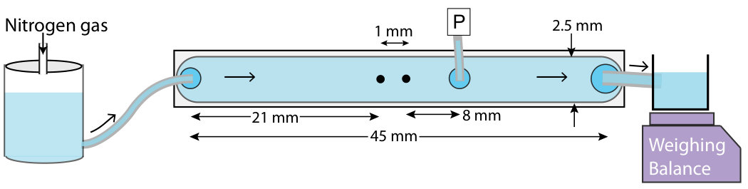 Figure 1
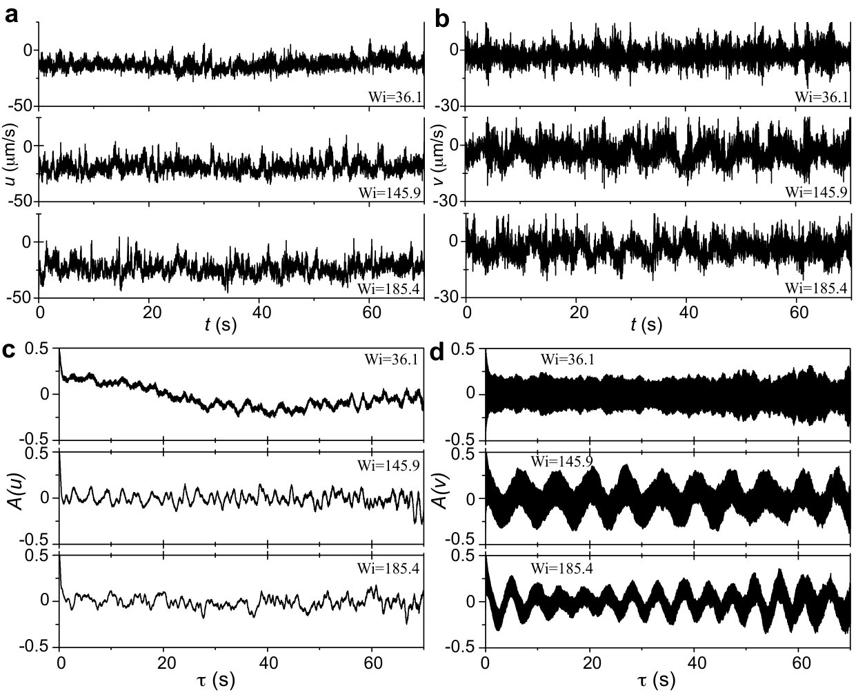 Figure 2
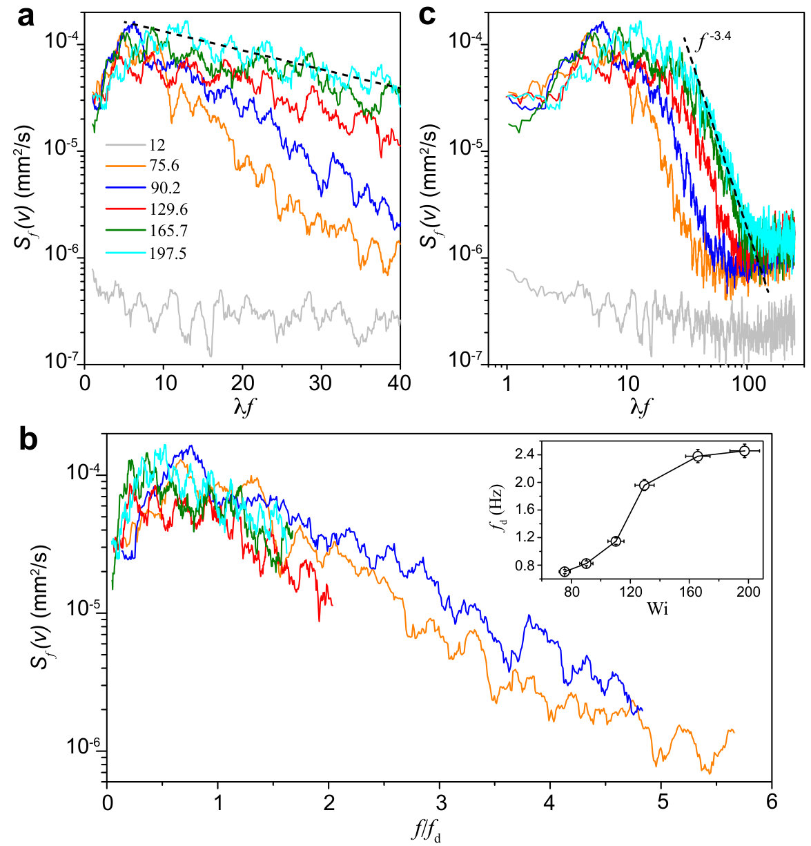 Figure 3
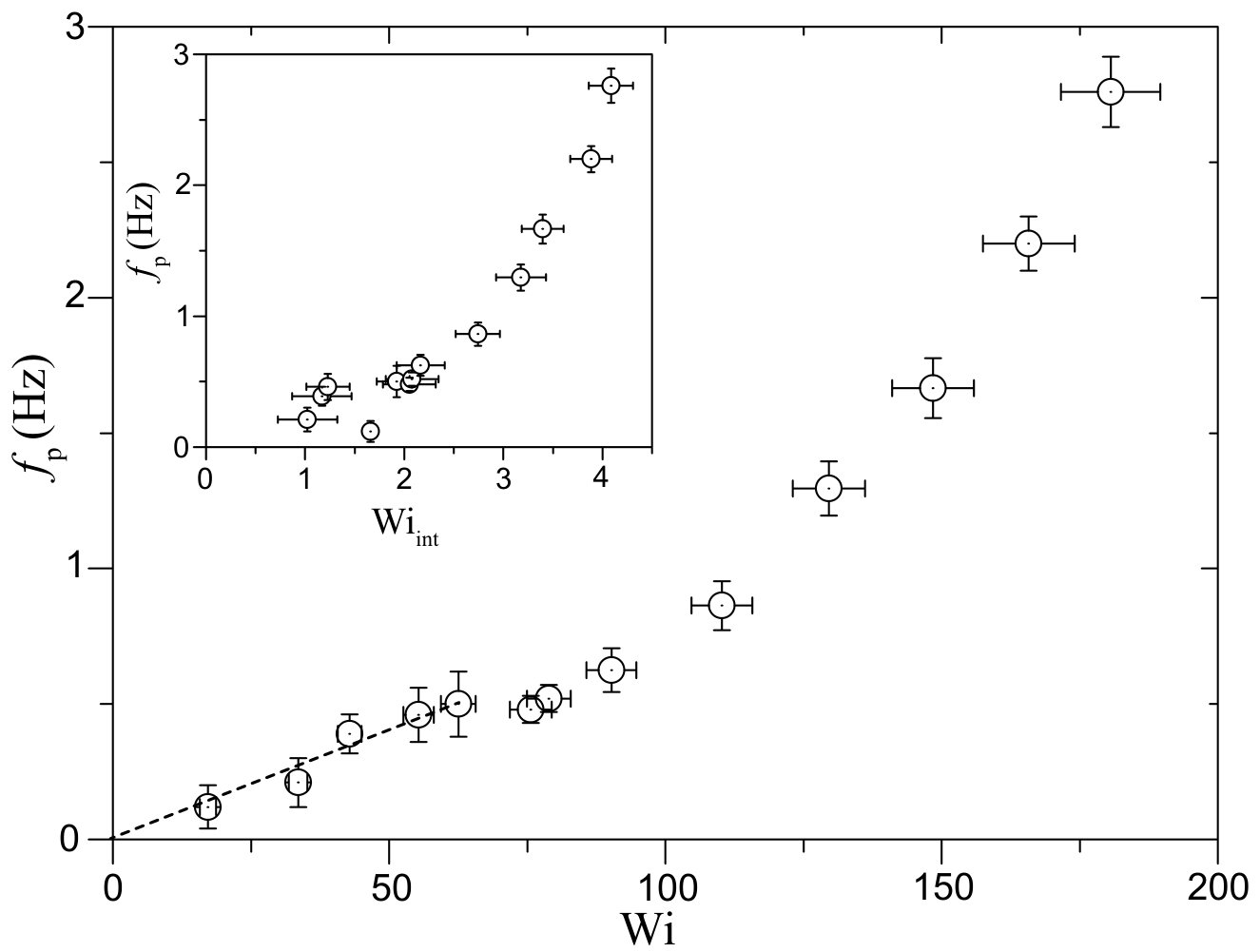 Figure 4
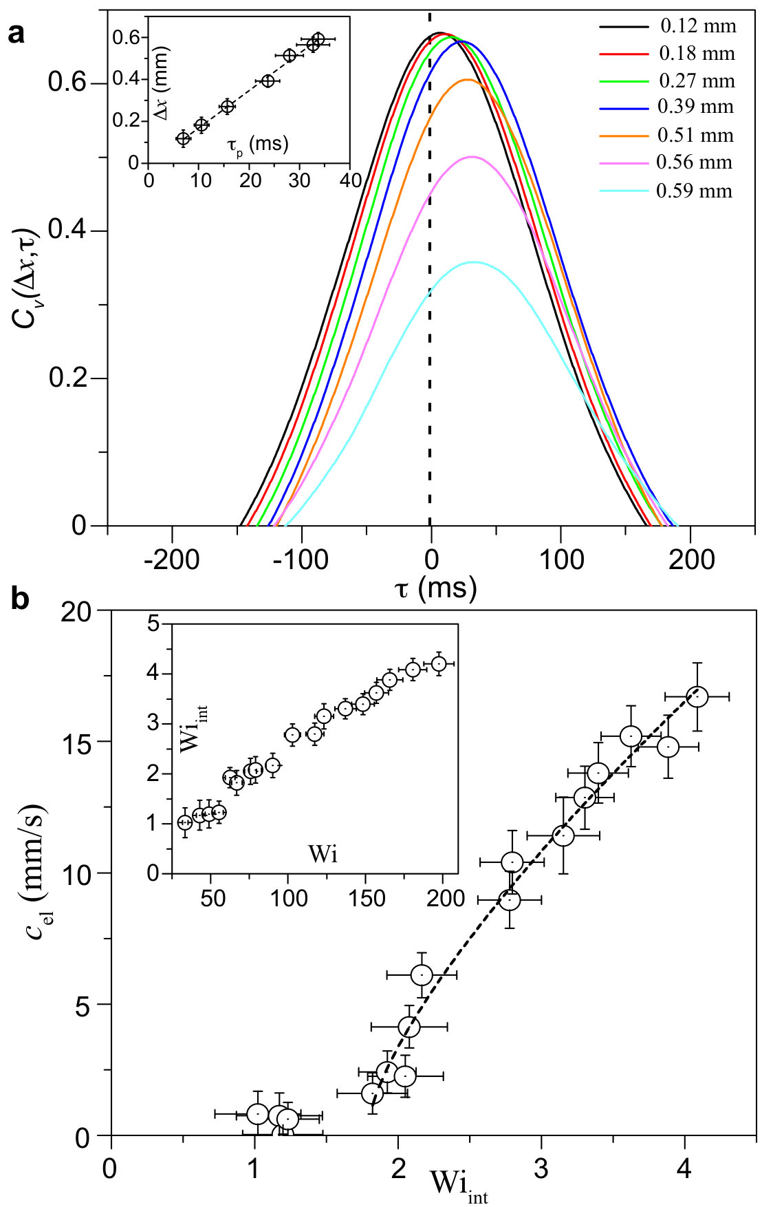 Figure 5
Peer Reviews
No public reviews on file for this paper yet. If you reviewed it on a platform where reviews are public (OpenReview, ICLR, NeurIPS, ICML), you can paste yours below so the community can read it here.
Videos
No videos yet. Explain this paper in a talk, walkthrough, or lecture? Add one.
Elastic Alfven waves in elastic turbulence
Atul Varshney1,2 and Victor Steinberg1,3
1Department of Physics of Complex Systems, Weizmann Institute of Science, Rehovot 76100, Israel
2Institute of Science and Technology Austria, Am Campus 1, 3400 Klosterneuburg, Austria
3The Racah Institute of Physics, Hebrew University of Jerusalem, Jerusalem 91904, Israel
Abstract
Speed of sound waves in gases and liquids is governed by medium compressibility. There exists another type of non-dispersive waves which speed depends on stress instead of medium elasticity. A well-known example is the Alfven wave propagating, with a speed determined by a magnetic tension, in plasma permeated by a magnetic field. Later, an elastic analog of the Alfven waves has been predicted in a flow of dilute polymer solution, where elastic stress engendered by polymer stretching determines the elastic wave speed. Here, we present quantitative evidence of elastic Alfven waves observed in elastic turbulence of a viscoelastic creeping flow between two obstacles hindering a channel flow. The key finding in the experimental proof is a nonlinear dependence of the elastic wave speed on Weissenberg number , which deviates from the prediction based on a model of linear polymer elasticity.
A small addition of long-chain, flexible, polymer molecules strongly affects both laminar and turbulent flows of Newtonian fluid. In the former case, elastic instabilities and elastic turbulence (ET) 1, 2, 3, 4, 5 are observed at Reynolds number and Weissenberg number , whereas in the latter, turbulent drag reduction (TDR) at and has been found about 70 years ago but its mechanism is still under active investigation 6. Here both and are defined via the mean fluid speed and the vessel size , and are the density and the dynamic viscosity of the fluid, respectively, and is the longest polymer relaxation time. ET is a chaotic, inertialess flow driven solely by nonlinear elastic stress generated by polymers stretched by the flow, which is strongly modified by a feedback reaction of elastic stresses 7. The only theory of ET based on a model of polymers with linear elasticity predicts elastic waves that are strongly attenuated in ET, but elastic waves may play a key role in modifying velocity power spectra in TDR 7, 8. Using the Navier-Stokes equation and the equation for the elastic stresses in uniaxial form of the stress tensor approximation, one can write the polymer hydrodynamic equations in the form of the magneto-hydrodynamic (MHD) equations 8. Then, by analogy with the Alfven waves in MHD 9, 10, one gets the elastic wave linear dispersion relation as with the elastic wave speed 7, 8 , where and are frequency and wavevector respectively, is the elastic stress tensor, and is the major stretching direction, similar to the director in nematics. Such an evident difference between the elastic stress tensor characterized by the director and the magnetic field that is the vector, however, does not alter the similarity between the elastic and Alfven waves, since only uniaxial stretching independent of a certain direction is a necessary condition for the wave propagation determined by the stress value 7.
A simple physical explanation of both the Alfven and elastic waves can be drawn from an analogy of the response of either magnetic or elastic tension on transverse perturbations and an elastic string when plucked. As in the case of elastic string, the director is sufficient to define the alignment of the stress. Thus, to excite either Alfven or elastic waves the perturbations should be transverse to the propagation direction, unlike longitudinal sound waves in plasma, gas, and fluid media 11. The detection of the elastic waves is of great importance for a further understanding of ET mechanism and TDR, where turbulent velocity power spectra get modified according to Ref. 7. Moreover, provides unique information about the elastic stresses, whereas the wave amplitude is proportional to the transversal perturbations, both of which are experimentally unavailable otherwise 8.
Numerical simulations of a two-dimensional Kolmogorov flow of a viscoelastic fluid with periodic boundary conditions reveal filamented patterns in both velocity and stress fields of ET 12. These patterns propagate along the mean flow direction in a wavy manner with a speed , nearly independent of . In subsequent studies, extensive three-dimensional Lagrangian simulations of a viscoelastic flow in a wall-bounded channel with a closely spaced array of obstacles show transition to a time-dependent flow, which resembles the elastic waves 13. Further, the elastic stress field around the obstacles demonstrates similar traveling filamental structures 12, 13 in ET, interpreted as elastic waves 7, 8. However, in both studies neither the linear dispersion relation nor the dependence of wave speed on elastic stressprimary signatures of the elastic waveswere examined. Moreover, was found to be close to the flow velocity, contradicting the theory 7, 8. Strikingly, an indication of the elastic waves, in numerical studies, originates from observed frequency peaks in the velocity power spectra above the elastic instability 12, 13. Analogous frequency peaks in the power spectra of velocity and absolute pressure fluctuations above the instability were also reported in experiments of a wall-bounded channel flow in a creeping viscoelastic fluid, obstructed by either a periodic array of obstacles 14 or two widely-spaced cylinders 15, 16. These observations were in agreement with numerical simulations 17 and were associated with noisy cross-stream oscillations of a pair of vortices engendered due to breaking of time-reversal symmetry.
Our early attempts to excite the elastic waves both in a curvilinear flow and in an elongation flow of polymer solutions at were unsuccessful 18. In the ET regime of the curvilinear channel flow, either an excitation amplitude was insufficient and/or an excitation frequency was too high. The reason we chose the elongation flow, realized in a cross-slot micro-fluidic device, is a strong polymer stretching in a well-defined direction along the flow. However, the elongation flow generated in the cross-slot geometry has the highest elastic stresses in a central vertical plane parallel to the flow in the outlet channelsanalogous to a stretched vertical elastic membrane. The transverse periodic perturbations in the experiment were applied in a cross-stream direction from the top wall 18, however a more effective method would be to perturb it in a span-wise direction that was difficult to realize in a micro-channel. A higher frequency range of perturbations, compared to that found in the current experiment, was used that lead to the wave excitation with wave numbers in the range of high dissipation.
Here we report the first evidence of elastic waves observed in elastic turbulence of a dilute polymer solution flow in a wake between two widely-spaced obstacles, hindering a channel flow. The central finding in the experimental proof of the elastic wave observation is a power-law dependence of on , which deviates from the prediction based on a model of linear polymer elasticity 7. The distinctive feature of the current flow geometry is a two-dimensional nature of the ET flow, in the mid-plane of the device, in contrast to other flow geometries studied earlier.
**Results
Flow structure and elastic turbulence.** The schematic of the experimental setup is shown in Fig. 1, where two-widely spaced obstacles hinder the channel flow of a dilute polymer solution (see Methods section for the experimental setup, solution preparation and its characterization). The main feature of the flow geometry used is the occurrence of a pair of quasi-two-dimensional counter-rotating elongated vortices, in the region between the obstacles, as a result of the elastic instability 15 at and ; and , where obstacles’ diameter and average flow speed are defined in Methods section. The frequency power spectra of cross-stream velocity fluctuations show oscillatory peaks at low frequencies 15, 16 below . Above the elastic instability, the main peak frequency grows linearly with , characteristic to the Hopf bifurcation 15. The two vortices form two mixing layers with a non-uniform shear velocity profile and with further increase of their dynamics become chaotic, exhibiting ET properties, with vigorous perturbations that intermittently destroy vortices 16 and seemingly excite the elastic waves. The ET flow in the region between the obstacles is shown through long-exposure particle streaks imaging in Supplementary Movies 1-3 19 for three different .
Characterization of low frequency oscillations. To investigate the nature of these oscillations we present time series of the streamwise and cross-stream velocity components and their temporal auto-correlation functions and in Fig. 2a-d. Distinct oscillations in contrary to weak noisy oscillations in indicate flow anisotropy. Further, the cross-stream velocity power spectra as a function of normalized frequency for five values in the ET regime are shown in log-lin and log-log coordinates in Figs. 3a and b, respectively. The power spectra exhibit the oscillation peaks at low frequencies up to with an exponential decay of the peak values (Fig. 3a). These low frequency oscillations look much more pronounced on a linear scale (Supplementary Fig. 1(a) 19). Further, these oscillations are also observed in the power spectra of pressure fluctuations versus , though not so regular (Supplementary Fig. 1(b) 19). The exponential decay of at implies that only a single frequency (or time) scale is identified for each (Fig. 3a). This frequency , for each , is obtained by an exponential fit to the data, i.e. . The variation of with is shown in the inset in Fig. 3b; it varies from 0.7 to 2.5 Hz in the range of from 75 to 200, which is comparable to oscillation peak frequency (Fig. 4) and larger than . Strikingly, on normalization of with for each , for all collapse on to each other (Fig. 3b). At higher frequencies up to , decay as the power-law with the exponent typical for ET 5 (Fig. 3c). Contrary to a general case, where the power-law decay of corresponding to ET 3, 4, 5 commences at , the low frequency oscillations cause the power-law spectra start to decay at higher frequencies , perhaps due to an additional mechanism of energy pumping into ET associated with the low frequency oscillations. In addition, exhibit the power spectra decay in the high frequency range with the exponent close to -3 (see the bottom inset in Fig. 2 in Ref. 16), characteristic to the ET regime 20. It should be emphasized that the power spectra of the streamwise velocity do not show the low frequency oscillations and decays with a power-law exponent .
Figure 4 shows the dependence of in a wide range of . The first elastic instability, characterized as the Hopf bifurcation, occurs at low , where grows linearly with \mathrm{Wi}$$-in accord with our early results 15. At higher in the ET regime, dependence becomes nonlinear at . In the inset in Fig. 4, we present the same data for as a function of . Here, the Weissenberg number of the inter-obstacle velocity field is defined as and is the time-averaged shear-rate in the cross-stream direction in the inter-obstacle flow region. The parameter is relevant to the description of elastic waves in ET flow between the obstacles’ region. The inset in Fig. 5b shows a linear dependence of on .
Dependence of elastic wave speed on . Figure 5a shows a family of temporal cross-correlation functions of between two spatially separated points, with their distance being , located on a horizontal line at for . A gaussian fit to in the vicinity of yields the peak value at a given . A linear dependence of on (e.g. Fig. 5a inset for ) provides the perturbation propagation velocity as . The variation of as a function of is presented in Fig. 5b together with nonlinear fit of the form , where mm s*-1*, , and onset value . The same data of is plotted against (see Supplementary Fig. 3 19) and fitted as that yields the onset value .
Discussion
In the light of the predictions 7, it is surprising to observe the elastic waves in the ET regime due to their anticipated strong attenuation. An estimate of the wave number from (Fig. 5b) and (Fig. 4) provides in the range between 0.63 and 1.3 (Supplementary Fig. 2 19). The corresponding wavelengths () are significantly larger than the inter-obstacle spacing mm. The spatial velocity power spectra is limited by a size of the observation window of about 0.7 mm that gives mm*-1*, much larger than the wave numbers calculated above. Thus, the low part of , where the elastic wave peaks can be anticipated, is not resolved by the spatial velocity spectra (Supplementary Fig. 4(b) 19). The power-law decay with is found at low followed by a bottleneck part and a consequent gradual power-law decay with an exponent at higher (Supplementary Fig. 4(b) 19), unlike , where the peaks appear at low and the steep power-law decay with the exponent at higher (see Fig. 3b). The spatial streamwise velocity power spectra , obtained at the same and near the center line , are similar to at low and decays gradually with exponent at higher (Supplementary Fig. 4(a) 19).
The observed nonlinear dependence of on differs from the theoretical prediction based on the Oldroyd-B model 7, 8. The expression for the elastic wave speed in the model 21 gives , where is the first normal stress difference. Then one obtains . First, is proportional to and second, the coefficient in the expression for the parameters used in the experiment is estimated to be mm s*-1*. Taking into account that the model 7, 8 and the estimate of elastic stress are based on linear polymer elasticity 21, whereas in experiments polymers in ET flow are stretched far beyond the linear limit 22, thus it is not surprising to find the quantitative discrepancies between them. Indeed, the value of the coefficient found from the fit ( mm s*-1*) and estimated theoretical value ( mm s*-1*) differ almost by a factor of two (see Fig. 5b). Moreover, for the maximal value of mm s*-1* (at ) obtained in the experiment, an estimate of elastic stress gives Pa that is lower but comparable with Pa obtained from the experiment on stretching of a single polymer T4DNA molecule at similar concentrations 22. Thus, both the dependence on and the coefficient value indicate that the Oldroyd-B model based on linear polymer elasticity cannot quantitatively describe the elastic wave speed and so the elastic stresses. Another aspect of this result is the Mach number ; the maximum value achieved in the experiment is , contrast to what is claimed in 23, 24 due to a wrong definition based on the elasticity instead of elastic stress used for the estimation of and .
We discuss two possible reasons related to the detection of the elastic waves. As indicated in the introduction, the key feature of the current geometry is a two-dimensional nature of the chaotic flow, at least in the mid-plane of the device (see Fig. 4SM in Supplemental Material of Ref. 16), that makes it analogous to a stretched elastic membrane. This flow structure is different from three-dimensional elastic turbulence in other studied flow geometries and thus may explain the failure in the earlier attempts to observe the elastic waves. Another qualitative discrepancy with the theory 7, 8 is the predicted strong attenuation of the elastic waves in ET. Below we estimate the range of the wave numbers with low attenuation for the elastic waves and compare with the observed values.
There are two mechanisms of the elastic wave attenuation, namely polymer (or elastic stress) relaxation and viscous dissipation 7, 8. The former has scale-independent attenuation , which at the weak attenuation satisfies the relation , and the latter provides low attenuation 25 at . The first condition leads to , where that provides a minimum wave number in the ET regime as for . The maximum value of follows from the second condition that gives at . Thus, one obtains in the ET regime for and therefore, the range of the wave numbers with the low attenuation is rather broad and lies far outside of the -range of and presented in Supplementary Fig. 4 19, where the range of the wave numbers of the elastic waves is not resolved. However, the range of the observed wave number of the elastic waves, shown in Supplementary Fig. 2 19, is sufficiently close to the estimated upper bound of .
Methods
Experimental setup. The experiments are conducted in a linear channel of , shown schematically in Fig. 1. The channel is prepared from transparent acrylic glass (PMMA). The fluid flow is hindered by two cylindrical obstacles of mm made of stainless steel separated by a distance of mm and embedded at the center of the channel. Thus the geometrical parameters of the device are , and (see Fig. 1). The longitudinal and transverse coordinates of the channel are and , respectively, with ()=() lies at the center of the upstream cylinder. The fluid is driven by gas at a pressure up to psi and is injected via an inlet into the channel.
Preparation and characterization of polymer solution. As a working fluid, a dilute polymer solution of high molecular weight polyacrylamide (PAAm, MDa; Polysciences) at concentration ppm (, where ppm is the overlap concentration for the polymer used 26) is prepared using a water-sucrose solvent with sucrose weight fraction of . The solvent viscosity, , at is measured to be in a commercial rheometer (AR-1000; TA Instruments). An addition of the polymer to the solvent increases the solution viscosity, , of about . The stress-relaxation method 26 is employed to obtain longest relaxation time () of the solution and it yields s.
Flow discharge measurement. The fluid exiting the channel outlet is weighed instantaneously as a function of time by a PC-interfaced balance (BA210S, Sartorius) with a sampling rate of and a resolution of . The time-averaged fluid discharge rate is estimated as . Thus, Weissenberg and Reynolds numbers are defined as and , respectively; here and fluid density Kg m*-3*.
Imaging system. For flow visualisation, the solution is seeded with fluorescent particles of diameter (Fluoresbrite YG, Polysciences). The region between the obstacles is imaged in the mid-plane via a microscope (Olympus IX70), illuminated uniformly with LED (Luxeon Rebel) at wavelength, and two CCD cameras attached to the microscope: (i) GX1920 Prosilica with a spatial resolution pixel at a rate of fps and (ii) a high resolution CCD camera XIMEA MC124CG with a spatial resolution pixel at a rate of fps, are used to acquire images with high temporal and spatial resolutions, respectively. We perform micro particle image velocimetry 27 (PIV) to obtain the spatially-resolved velocity field in the region between the cylinders. Interrogation windows of pixel2 () for high temporal resolution images and pixel2 () for high spatial resolution images, with overlap are chosen to procure .
The reference list from the paper itself. Each links out to its DOI / PubMed record.
- 11 Larson, R. G. Instabilities in viscoelastic flows. Rheol. Acta 31 , 213–263 (1992).
- 22 Shaqfeh, E. S. G. Purely Elastic Instabilities in Viscometric Flows. Annu. Rev. Fluid Mech. 28 , 129–185 (1996).
- 33 Groisman, A. and Steinberg, V. Elastic turbulence in a polymer solution flow. Nature 405 , 53–55 (2000).
- 44 Groisman, A. and Steinberg, V. Efficient mixing at low Reynolds numbers using polymer additives. Nature 410 , 905–908 (2001).
- 55 Groisman, A. and Steinberg, V. Elastic turbulence in curvilinear flows of polymer solutions. New J. Phys. 6 , 29 (2004).
- 66 Toms, B. A. Some Observation on the Flow of Linear Polymer Solutions Through Straight Tubes at Large Reynolds Numbers. volume 2, 135–141, (1948).
- 77 Balkovsky, E., Fouxon, A., and Lebedev, V. Turbulence of polymer solutions. Phys. Rev. E 64 , 056301 (2001).
- 88 Fouxon, A. and Lebedev, V. Spectra of turbulence in dilute polymer solutions. Phys. Fluids 15 , 2060–2072 (2003).