Dwell-time control sets and applications to the stability analysis of linear switched systems
Francesco Boarotto, Mario Sigalotti (CaGE, LJLL)

TL;DR
This paper extends control set theory to dwell-time constrained inputs, enabling stability analysis of linear switched systems and characterization of invariant measures using a modified control set approach.
Contribution
It introduces a new definition of control sets for dwell-time inputs, facilitating stability analysis and measure support characterization in switched systems.
Findings
Characterized maximal Lyapunov exponent using periodic angular trajectories.
Provided a framework for analyzing invariant measures in dwell-time switched systems.
Extended control set theory to non-concatenable input classes.
Abstract
We propose an extension of the theory of control sets to the case of inputs satisfying a dwell-time constraint. Although the class of such inputs is not closed under concatenation, we propose a suitably modified definition of control sets that allows to recover some important properties known in the concatenable case. In particular we apply the control set construction to dwell-time linear switched systems, characterizing their maximal Lyapunov exponent looking only at trajectories whose angular component is periodic. We also use such a construction to characterize supports of invariant measures for random switched systems with dwell-time constraints.
Click any figure to enlarge with its caption.
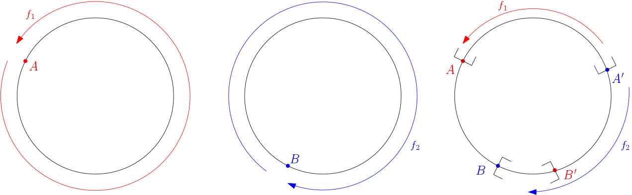 Figure 1
Peer Reviews
No public reviews on file for this paper yet. If you reviewed it on a platform where reviews are public (OpenReview, ICLR, NeurIPS, ICML), you can paste yours below so the community can read it here.
Videos
No videos yet. Explain this paper in a talk, walkthrough, or lecture? Add one.
Taxonomy
TopicsStability and Control of Uncertain Systems · Advanced Differential Equations and Dynamical Systems · Advanced Control Systems Optimization
Dwell-time control sets and applications to the stability analysis of
linear switched systems
Francesco Boarotto
Dipartimento di Matematica Tullio Levi-Civita, Università degli studi di Padova, Italy
and
Mario Sigalotti
Inria Paris & Laboratoire Jacques-Louis Lions, Sorbonne Université, Université Paris-Diderot SPC, CNRS, Inria, 75005 Paris, France
Abstract.
We propose an extension of the theory of control sets to the case of inputs satisfying a dwell-time constraint. Although the class of such inputs is not closed under concatenation, we propose a suitably modified definition of control sets that allows to recover some important properties known in the concatenable case. In particular we apply the control set construction to dwell-time linear switched systems, characterizing their maximal Lyapunov exponent looking only at trajectories whose angular component is periodic. We also use such a construction to characterize supports of invariant measures for random switched systems with dwell-time constraints.
Key words and phrases:
Linear switched systems, control sets, Lyapunov exponents, invariant measures.
2010 Mathematics Subject Classification:
93C30, 37H15, 37L40
The authors have been supported by the ANR SRGI (reference ANR-15-CE40-0018). F.B. is also supported by University of Padova STARS Project “Sub-Riemannian Geometry and Geometric Measure Theory Issues: Old and New”. M.S. warmly thanks Fritz Colonius for the exchanges about the results in the paper and for his many useful suggestions.
1. Introduction
Control sets are geometric objects reflecting the structural properties of the family of all reachable sets of a given control system [14]. They also happen to be a very helpful geometric tool for investigating the stability properties of linear switched systems. For a linear switched system on with set of modes , one can consider the induced switched system on the projective space obtained by looking at the angular component of the state. Under the assumption that the set of projected modes, seen as vector fields on , satisfies the Lie algebra rank condition, there exists a unique nonempty set such that the closure of the reachable set from any point in is equal to itself. Moreover, the set , which is called invariant control set, has nonempty interior in and is contained in the closure of the reachable set from any other point in . An important application of this property is a useful characterization of maximal and minimal Lyapunov exponents. Under the Lie algebra rank condition mentioned above, indeed, these exponents that characterize the asymptotic behavior of the system, and in particular its stability, can be computed by looking solely at periodic inputs which generate trajectories whose angular components are also periodic. The idea of looking at the Lyapunov exponents associated with the restricted class of periodic trajectories has been introduced in [3] in order to relate the asymptotic stability of linear stochastic systems with the behavior of their large deviations, measured in terms of -th mean Lyapunov exponents. The characterization in terms of periodic trajectories turns out to be useful also to prove the continuity of Lyapunov exponents (see [13] and also [11], where invariant control sets are used to prove continuity for Lyapunov exponents associated with systems subject to persistently exciting inputs).
Another important property of control sets, which is the original motivation for their introduction in the literature [2], is that they allow to characterize supports of invariant measures for piecewise deterministic Markov processes on compact manifolds [7]. (See also [8], where some ad hoc construction of control set is developed for two-dimensional linear switched systems.)
A limitation of the control set approach is that it has been developed for the point of view of controllability theory, hence control signals are allowed to vary arbitrarily as time goes. This paper, motivated by the study of switched systems, aims at presenting a first extension of the theory of control sets to classes of input signals with restrictions on the switching rule. The most studied of these classes consists of signals satisfying dwell-time constraints, i.e., the interval between two successive switching times has length larger than a given positive constant. The most important structural difference between the classes of dwell-time and arbitrary switching signals is that the former is not closed under concatenation, in the sense that concatenating two pieces of switching signals satisfying the dwell-time constraint does not necessarily yield a dwell-time signal. Such a lack of concatenability induces the most relevant technical difficulties that we are lead to tackle in this paper.
Our contribution is based on a new suitable notion of control set adapted to the dwell-time setting. Instead of basing the construction on reachable sets as in the case of arbitrary switching, we restrict the attention to points which can be attained at the final time of a concatenation of constant signals of length larger than the dwell-time. This leads to a inner estimate of the reachable set, not necessarily connected, but which is shown to be sufficient to yield a proper notion of dwell-time control set. The latter shares most existence, uniqueness, and topological properties with its counterpart for arbitrary switching. (Similar results could have been obtained following the approach in [23], at least when the Lie algebra generated by the modes of the switched system is finite-dimensional.) As a consequence, in the linear case, we extend the results of [13] on the characterization of the maximal Lyapunov exponent by trajectories with periodic angular component. We also describe the support of invariant measures for random switched systems with dwell-time. Most of the paper deals with general systems on a (mostly compact) manifold. The results for linear switched systems are then obtained by considering the induced system on the projective space.
While proving these results we also partially extend the results known for arbitrarily switching, in particular by removing the Lie algebra rank condition from the characterization of Lyapunov exponents in terms of trajectories with periodic angular components. This is made possible by a new result dealing with the representation of Lie groups, which ensures that the action of the group of flows associated with the lifted linear switched system has at least one compact orbit on (or ). This result, which we believe to be of independent interest, seems not to be present in the literature. We are indebted to Uri Bader and Claudio Procesi for their crucial help in providing its proof (presented in the appendix).
The paper is organized as follows. In Section 2 we state the main results on linear switched systems contained in the paper. Section 3 contains the definition and construction of dwell-time control sets, establishing their basic properties and illustrating them on a simple example on the projective circle. In Section 4 dwell-time control systems are specified to the case of linear switched systems and their induced dynamics on the projective space. In particular, we show in Theorem 24 that if we restrict a projected linear switched systems to a compact orbit of the corresponding matrix Lie group, then the restricted system admits an unique invariant dwell-time control set (where invariance is defined in a suitable way that takes into account the dwell-time constraint). Based on this result, we prove in Theorem 29 that the maximal Lyapunov exponent can be achieved looking only at trajectories with periodic angular component. Finally, in Section 5 we relate dwell-time control sets and the support of invariant measures for piecewise deterministic dwell-time random processes.
2. Linear switched systems: main results
We present in this section the main results that we obtain for linear switched systems, simplifying when necessary the assumptions and the notations with respect to the following sections, in order to avoid technicalities.
Given an integer , a set of matrices, and a scalar , we consider on the system
[TABLE]
with in the set of all piecewise constant functions from to such that
[TABLE]
where is the (possibly finite) increasing sequence of discontinuities of . A solution to (2.1) is characterized by and the initial condition , and is denoted by .
Notice that the dwell-time condition (2.2) is equivalent to asking that , where is the function computing the lower bound of the distance between distinct points of a subset of .
For every , define the reduced reachable set from
[TABLE]
For the case , the constraint is empty and the set is the usual reachable set from for system (2.1), in which is seen as a piecewise constant control with values in . For , the constraint does play a role. The reduced reachable set is defined in this way in order to ensure, in particular, the property that
[TABLE]
2.1. Closed orbits for zero-dwell systems
A technical result that we use several times in the paper is the following.
Proposition 1**.**
Let and consider a set of matrices such that if and only if . Then there exists such that the set
[TABLE]
is compact.
The above result can be deduced from the following property of the actions of linear Lie groups.
Theorem 2**.**
Let be a connected Lie subgroup of . Then the action
[TABLE]
induced by on the -dimensional unit sphere , admits at least one closed orbit in .
The proof of the theorem is based on rather different arguments from those developed in the rest of the paper and is postponed to the appendix.
2.2. Periodization of trajectories
Let the set of matrices be bounded. The maximal Lyapunov exponent for (2.1) is defined as
[TABLE]
The goal of periodization is to offer a way to approximate by solving finite-horizon maximization problems. In order to do so, instead of maximizing over all trajectories with and , we might restrict our attention to those for which there exists such that is -periodic and is parallel to . Let us define by taking the sup in (2.4) restricted to these trajectories (see Section 4.4 for a detailed definition). Then clearly . In the case Colonius and Kliemann proved in [13] that the two quantities are actually equal, under the assumption that satisfies the Lie algebra rank condition on , that is, if the family of vector fields on the projective space induced by the elements of satisfies the Lie algebra rank condition. We extend their result by proving equality for every and removing the Lie algebra rank condition assumption.
Theorem** (Theorem 29).**
Let and consider a bounded set of matrices. Then .
2.3. Support of invariant measures
Consider now the case where is finite and the switching signal is a random variable. In order to guarantee that the dwell time-condition is verified, we assume that the switching times are independent random variables with identical probability distributions having support in . The probability of switching from one element of to another is encoded by a stochastic matrix. Under these hypotheses, it is possible to associate with the random switching system a probabilistic maximal Lyapunov exponent , which is almost surely attained by a trajectory of the system. (For details, see Section 5 and, in particular, Section 5.4.)
We then have the following.
Proposition** (Proposition 38).**
Let be finite and assume that it satisfies the Lie algebra rank condition on . For every , let be the projection on of for any vector projecting to . Set . Then there exists a probability measure on with
[TABLE]
absolutely continuous with respect to the Lebesgue measure, and such that
[TABLE]
3. Dwell-time control sets
We introduce in this section a general construction of control sets in the framework of nonlinear switching systems with a dwell-time constraint. In analogy with [14], we are going to establish the existence and some crucial geometric properties of these sets that we will extensively use later on in this paper, in particular for studying stability properties of switched systems with dwell-time.
3.1. Krener accessibility theorem with dwell-time constraints
Let be a -dimensional manifold and any nonempty set. We consider the control system
[TABLE]
where is such that is a smooth complete vector field for every and
[TABLE]
Let us denote by the function associating with the length of the time-interval on which is defined. We write for the trajectory of (3.1) starting at a point , and driven by the control on the time-interval . Let, moreover,
[TABLE]
and denote by the Lie algebra of vector fields on generated by (with respect to the Lie bracket operation).
An assumption that we will require for several results is that
[TABLE]
which is known as the Lie algebra rank condition. Here denotes the evaluation of at , that is, .
Definition 3**.**
Let . Then the concatenation is the piecewise constant function defined on by
[TABLE]
Definition 3 immediately extends to an arbitrary finite number of elements of .
Definition 4**.**
Let . Let us consider the subset of defined by
[TABLE]
In particular, . When the parameter is positive, it is commonly referred to as the dwell-time. Dwell-time constraints are used to model systems where, for technological, safety, or other reasons, the actuation of each control value cannot last less than a common bound .
Let us define
[TABLE]
that is, is the subset of diffeomorphisms of given by the collection of all the flows associated with controls in . Observe that admits the following alternative characterization
[TABLE]
Notice that has the semigroup property. Indeed, for every two elements , their composition is again an element of .
Definition 5** (Dwell-time attainable set).**
For every , , and , we set
[TABLE]
Notice that , where stands for the set . The semigroup property of implies that is dwell-time positively invariant, according to the following definition.
Definition 6**.**
A set is said to be dwell-time positively invariant if for every .
The following is an adaptation of the well-known Krener’s theorem to our current situation, that is, in presence of a dwell-time constraint.
Proposition 7**.**
Assume that (H) holds true. Then, for every and , .
Proof.
Fix and let . Since , there exists such that . For any we have
[TABLE]
where we set for some to be fixed later. Next, if , there exist and such that , for otherwise would be of dimension one, and (H) would be violated. Notice moreover that is still true if we vary in a small neighborhood. Then, for any , we compute
[TABLE]
The two tangent vectors at are linearly independent, since is a diffeomorphism of the tangent space. Again, if , we set , and, up to eventually modifying , we can find such that
[TABLE]
for otherwise would be contained in the tangent plane to the surface parameterized by (with in a neighborhood of ) and (H) would not hold. Repeating the argument above, suppose that and that at the -th step we define
[TABLE]
Then, up to slightly modifying , we can find such that
[TABLE]
Differentiating at zero the map
[TABLE]
we find that
[TABLE]
for . The differential of (3.8) is then of maximal rank locally at and the claim is proved after steps. ∎
Remark 8*.*
The proof of Proposition 7 actually shows that if (H) holds true, then, for every and there exist and such that is a local diffeomorphism at .
Proposition 9**.**
Let and
[TABLE]
be a local diffeomorphism at . Let . Then
[TABLE]
is also a local diffeomorphism at .
In particular, there exist an arbitrarily small neighborhood of in and , neighborhoods of , , respectively, such that for every and there exists such that .
Proof.
By assumption (compare with (LABEL:eq:family)), the vector fields appearing in the definition of satisfy the relation
[TABLE]
On the other hand, differentiating at [math] with respect to , , the map
[TABLE]
we obtain
[TABLE]
To see that the collection of vectors obtained in (3.13) is a basis of , it is sufficient to observe that they can be mapped to the collection appearing in (3.12) applying the push-forward . Since this latter family is a basis of , then is a local diffeomorphism at .
The last part of the statement follows by a standard compactness/continuity argument. ∎
Combining Remark 8 and Proposition 9 yields the following.
Corollary 10**.**
Assume that (H) holds true. Then, for every and , there exist with and a neighborhood of in such that for every there exists with and .
3.2. Control sets
Let us denote by the set of all piecewise constant functions such that there exists for which for every . With a slight abuse of notation, given (respectively, ) and (respectively, ), we say that is in (respectively, is in ) if (respectively, ) does.
A special role in what follows is played by those times in at which a signal is split into two subsignals which both satisfy the dwell-time condition. Such times are interesting because they can be used to modify by concatenating one of the subsignals with any other dwell-time signal. Such partial concatenability allows to prove the interesting properties that we seek to bring to light in control sets.
Definition 11**.**
A subset is said to be a dwell-time control set (-CS, for short) for system (3.1) if it satisfies the following conditions:
- (i)
For every there exists such that for all for which both is in and is in ;
- (ii)
For every , one has that ;
- (iii)
is maximal with these properties, i.e., if satisfies both (i) and (ii), then .
Moreover, a -CS is said to be an invariant -CS (-ICS, for short) if for every .
Remark 12*.*
Observe that, if is a subset of such that
[TABLE]
then automatically is a -ICS. Moreover, if (H) holds true, then any -ICS is closed. Indeed, consider a -ICS and let us prove that satisfies (3.14). The conclusion then follows by maximality. It is clear that for every , the set (and hence ) is contained in . In order to conclude, fix and let us notice that it is enough to show that intersects , since for every we have . Thanks to Remark 8 and Proposition 9, there exists such that covers a neighborhood of . Since, moreover, is in , we indeed have that intersects .
Remark 13*.*
Observe that if (H) holds true then contains at most countably many distinct -ICS. Indeed, admits a countable dense subset . Let be any -ICS. Then is characterized by (3.14) according to Remark 12. By Proposition 7, , hence there exists such that is in . But then . The family of all -ICS is therefore contained in .
Our first result on control sets is an existence property for invariant dwell-time control sets when is compact.
Theorem 14**.**
Let be compact. For each there exists a nonempty -ICS contained in . If, moreover, (H) holds true, then has nonempty interior.
Proof.
Let . Consider the collection . Then is nonempty, and all elements of are dwell-time positively invariant, since
[TABLE]
To check this, we let , for some . We need to prove that . Let be any neighborhood of . Since , then, for any neighborhood of , . We choose so small that , and then for any , we have that , since .
Now observe that is a partially ordered (with respect to the inclusion) collection of nonempty compact sets. The Cantor intersection theorem implies then that every descending chain is such that . Therefore, thanks again to (3.15), every chain has a lower bound of the form , for some .
The dual form of Zorn’s lemma applies, and yields that has a minimal element of the form , for some . In particular, is dwell-time positively invariant. By Remark 12, in order to prove that is a -ICS it remains to show that for all . Since is closed and dwell-time positively invariant, then . Equality then follows from the minimality property of .
Finally, Proposition 7 implies that has nonempty interior whenever (H) holds true. ∎
3.2.1. Properties of dwell-time control sets
Lemma 15**.**
Let be a subset of which is maximal with respect to property (ii) in Definition 11. Let and be such that . Then for all such that both and .
Proof.
Let us write for . It suffices to prove that for every such that both and , and every , both and . Indeed if this were true and , then would be a set strictly larger than that satisfies (ii) in Definition 11.
To check the second assertion, fix a neighborhood of . Then there exists a neighborhood of such that in for all . Since , for every we have that , and then there exists with . We concatenate and on to see that and , so we are done. The other assertion is easier, for it suffices to observe that , as by assumption. ∎
Lemma 16**.**
Let be a subset of that is maximal with respect to property (ii) in Definition 11. Assume that . Then is a -CS.
Proof.
It is sufficient to show that, for every , there exists such that for all such that is in and in .
Pick and fix two nonempty open subsets of such that . Applying twice property (ii) in Definition 11 , there exist , , and such that and . Up to restricting and , we can assume that . Applying iteratively property (ii) in Definition 11, we select a sequence such that for odd and for even, and a sequence in such that for every and for odd. Notice that . Hence, the concatenation of all is an element of , which we denote by .
Finally, if is such that both is in and in , then let be such that and notice that is in . Applying Lemma 15 with , we deduce that is in . Then is a -CS. ∎
Lemma 17**.**
Let (H) hold true and assume that is a -ICS. Then
- (i)
;
- (ii)
* is dwell-time positively invariant;*
- (iii)
There exists an open and dense subset of such that ;
- (iv)
There exists an open and dense subset of such that for all .
Proof.
Let us prove (i). Recall that by Proposition 7. The inclusion of in is obvious from Remark 12. As for the reverse inclusion, let us choose and any neighborhood of . We need to show that
[TABLE]
Using Proposition 7 we first deduce that there exists a nonempty open set contained in . Since , we have that is contained in . Let . By definition of -ICS, , and we pick . Hence , for some . Since is open, we can find a sufficiently small neighborhood of such that is a neighborhood of entirely contained in . Then is a nonempty open set in , in particular it is contained in , and (3.16) is proved.
As for (ii) we proceed as follows. Let and observe that since is dwell-time positively invariant, then is contained in . Since, moreover, is a diffeomorphism, then is open and hence contained in .
Consider now point (iii). Let be any nonempty open set in . We should prove that has nonempty interior. Fix some . According to Remark 8, there exist and such that is a local diffeomorphism at . Notice that
[TABLE]
is in and select such that . Thanks to Proposition 9, there exist , neighborhoods of respectively, such that for every and there exists such that
[TABLE]
Up to reducing and , we can assume that . We now complete the proof of (iii) by showing that is also contained in . Indeed, for any and there exist and such that and
[TABLE]
Hence, is in and maps to .
Let us finally prove (iv). Let be the union of all sets as in (iii). Then is dwell-time positively invariant, since for every as in (iii) and every , is also as in (iii). Hence, for , which in turn is contained in because of (iii). We conclude that , as required. ∎
Applying the previous results to the case where is compact, we can strengthen the conclusions of Remark 13 under the compactness assumption.
Proposition 18**.**
Let be a compact manifold and assume that (H) holds true. Then there exist finitely many distinct -ICS on .
Proof.
Reasoning by contradiction and following Remark 13, let be the countable collection of all distinct -ICS on . For each , consider the open and dense subset constructed as in point (iv) of Lemma 17. For every let us choose an element . Up to selecting a subsequence, still denoted by , we may assume that there exists .
Using Theorem 14, let us consider a -ICS and, accordingly, the open and dense set contained in . Then there exist and such that . Fix and neighborhoods of and respectively, such that . For large enough, . Then is an element of for large enough.
In particular, for every such , the inclusion
[TABLE]
holds true. Taking the closures on both sides of (3.17), we deduce that . The maximality property of (point (iii) in Definition 11) then implies that for every large enough, leading to a contradiction. ∎
Example 1*.*
Let us consider, on the one-dimensional projective space , two vector fields as in Figure 1.
The vector field has a single equilibrium and its trajectories outside turn counterclockwise, while has a single equilibrium different form and its trajectories outside turn clockwise. Each of the vector fields and can be obtained, for instance, by projecting on a linear dynamics conjugate to the one of the double integrator
[TABLE]
Fix a dwell-time and consider the family . Define the points and by the relations
[TABLE]
In what follows, the symbol denotes the closed arc connecting to in the clockwise direction. We claim that there exists a unique -ICS associated with , given by the union . In order to check it, first notice that is positively invariant for , is positively invariant for , and
[TABLE]
Let us show now that, for every , we have . To see this notice that as . Then we can reach from any point in the interior of (and in particular we can get as close as we want to the two boundary points) by taking large and then applying during a time larger than . Taking large and applying again for a time larger than , we can reach any point in the interior of , proving that contains . The symmetric argument starting from some point of concludes the proof of the fact that is a -ICS. The uniqueness of follows from the fact that, by dwell-time invariance, any -ICS must contain the global attractive equilibria for and , that is, and .
Notice that is connected (and actually equal to ) for small and not connected for large. Consider the critical situation, that is, the value of for which . In this case coincides with the arc . We claim that, in this case, the set of point (iv) in Lemma 17 is . Indeed, can be reached only by starting either at or . Since these points are equilibria, they cannot be reached using the semigroup as soon as we start within . This example shows, in particular, that may be different from the interior of the corresponding -ICS, in contrast with the case (see [14, Theorem 3.1.5]).
4. Applications to linear switched systems
4.1. The maximal Lyapunov exponent of a linear switched system
Let be a bounded set of matrices, playing the role of the control set in the previous section, and for denote by and the sets of piecewise constant signals with values in and dwell-time , in analogy with the sets and introduced earlier. We specify the notation to the set in order to stress that the vector fields considered here are linear and that they are identified with the corresponding matrices. The associated system is
[TABLE]
We call () a switched system, in order to stress that we focus on the uniform asymptotic properties of its dynamics, looking at as a switching signal rather than as a control law. Following the usual switched systems terminology, we refer to each element of as a mode of ().
For every we denote by the fundamental matrix of (), that is, the solution to
[TABLE]
It is immediate to see that is the unique solution to () with and that .
The boundedness of the set ensures that the trajectories of system () have at most exponential growth with a common upper bound on their growth rates. The lower of such upper bounds is the object of the following definition.
Definition 19**.**
Given and a bounded set , the uniform exponential rate and the maximal Lyapunov exponent are defined, respectively, by
[TABLE]
The definition is independent of the choice of the norm on , since all norms on a finite-dimensional vector space are equivalent.
Since () can be seen as a linear flow on a vector bundle, we have
[TABLE]
for every choice of and [14].
4.1.1. Reduction to an irreducible component
We recall in this section how to reduce the stability analysis of () to the case in which the set is irreducible, i.e., when there exist no proper subspaces of that is invariant for all matrices in .
The next result relates the properties of a reducible switched system to those of lower dimensional irreducible ones. For a discussion, see, for instance, [12, Section IV.B].
Proposition 20**.**
Let be bounded. Then there exist , , and two subspaces of of dimensions and respectively, each of them invariant for all matrices in , such that for every basis of for which is a basis of , representing for every matrix the linear operator in the basis as the matrix
[TABLE]
where each is a matrix, we have that and is irreducible. Moreover, and can be chosen so that either or .
4.2. Projected switched systems and their orbits
It is an old idea to describe the nonzero trajectories of a linear system in coordinates . The advantage is that the dynamics of the angular part follow a well-defined switched system on a compact manifold. In order to formalize this idea, we associate with () the following projected switched system.
Definition 21**.**
Denoting by the canonical projection of onto its associated projective space and setting , we define the nonlinear projected switched system
[TABLE]
where for any matrix we denote by the projection of the vector field onto .
Using the local identification , () can be rewritten as
[TABLE]
The system semigroup (3.3) associated with () is given by
[TABLE]
We identify with a semigroup both of and of the group of diffeomorphisms of . It is also useful to introduce the system group
[TABLE]
It might be worth noticing that would not be not affected if we added the dwell time constraint , . Indeed, for every and every , we have , and if , then .
In addition to the previous notations, for every we denote the orbit of through by
[TABLE]
The following result is a consequence of the analytic version of the Orbit Theorem [22, 24].
Proposition 22**.**
Let be a subset of . Then the following properties hold true:
- i)
For every the orbit is an immersed submanifold of . Moreover, for every , one has
[TABLE]
where denotes the set of vector fields on defined by
[TABLE] 2. ii)
There exists for which the orbit is an embedded compact submanifold of ; 3. iii)
If is irreducible then for every and every proper subspace the orbit is not contained in .
Proof.
Point i) is a direct consequence of the analytic version of Orbit Theorem by Nagano and Sussmann, since is an analytic manifold and each of the vector fields is analytic on .
As for point ii), the existence of such that is compact follows directly from Theorem 2, since is a Lie subgroup of (see, e.g., [17, Propositions 2.6, 2.7]). We then use the general fact that orbits which are closed as subsets of the ambient manifold are not only immersed but also embedded submanifolds (see [9, Corollary 2.5]).
We are left to prove iii). Assume by contradiction that there exists and a proper subspace such that . Let
[TABLE]
Then is contained in and is invariant for all matrices in . Since is a proper subspace and , this contradicts the irreducibility of . ∎
Proposition 23**.**
The interior of for the relative topology on , seen as an immersed submanifold of , is nonempty, that is,
[TABLE]
Proof.
Consider the system
[TABLE]
where is seen as a control law. Such a system satisfies hypothesis (H) on : indeed, by the Orbit Theorem, for every the tangent is equal to . (Notice that is an analytic vector field on for every .)
We then apply Proposition 7 to system (4.9), to conclude that the attainable set from the identity map has nonempty interior in as soon as . This concludes the proof, since contains . ∎
4.3. Uniqueness of the -ICS in the projective space
The main result of this section is Theorem 24 stated below, which extends to the dwell-time setting the uniqueness result for [math]-ICS of linear systems and the characterization of such a unique [math]-ICS (cf. [3]). Let us mention that similar uniqueness results have been obtained (in the case ) for systems on Lie groups with a suitably defined linear structure (see [4]).
Theorem 24**.**
Assume that is an irreducible subset of . Let be such that the orbit is closed. Then there exists a unique -ICS for system () contained in . Moreover,
[TABLE]
and , that is, has nonempty interior in the orbit topology.
Remark 25*.*
In the case where satisfies assumption (H), then is irreducible and . In this case Theorem 24 implies that system () has a unique -ICS in .
Before providing a proof for Theorem 24, inspired by the one of [3, Theorem 3.1], let us present a couple of preliminary lemmas.
Lemma 26**.**
Let be such that the orbit is closed, and let us define
[TABLE]
Assume that . Then is a -ICS for system () on .
Proof.
Since for every by construction, it is sufficient to show that for every .
Fix , , and let us prove that . By construction of , is in for every . But this implies that also is in for every , that is, . ∎
Given a linear subspace of , we can identify any isomorphism of with a collineation of , i.e., a diffeomorphism of , the projective space of . Let us endow the group of collineations of , denoted by , with the topology of the uniform convergence.
We recall that a matrix is semisimple if and only if it admits a diagonal complex Jordan normal form.
Lemma 27**.**
Let be an irreducible subset of and be semisimple. Let be the linear subspace spanned by the eigenspaces of corresponding to eigenvalues having maximal real part. Fix . Then
[TABLE]
is nonempty for every in a dense subset of . Assume moreover that is such that is closed. Then is path-connected.
Proof.
Fix a system of coordinates in such that is in diagonal block form with blocks of size or and every block of size has the form with . For the Euclidean structure associated with these coordinates, the orthogonal complement is spanned by the eigenspaces of corresponding to eigenvalues whose real part is not maximal.
Consider a nonempty open subset of . Notice that
[TABLE]
only if . Since is an analytic manifold and is nonempty and open, we deduce that , which contradicts point iii) of Proposition 22. This proves the first part of the statement.
Assume now that is closed. In particular, is also closed. Up to reordering the coordinates of , we can assume that
[TABLE]
where denotes the dimension of . Endow with the homogeneous coordinates associated with . Then, given , we can write as . Since is semisimple, Dirichlet’s approximation theorem implies that there exists an unbounded sequence satisfying
[TABLE]
Hence,
[TABLE]
Fix and in . Consider an analytic path such that , , and for every . We claim that , which is defined for such that , admits a continuous extension . Indeed, if is such that , let be the smallest positive integer such that the -th derivative is not in . Such exists by analyticity of . Hence is an isolated time for which and
[TABLE]
Hence, setting we obtain a continuous extension of . The values of are also in , since the latter is closed and because of (4.11). This concludes the proof of the lemma. ∎
Proof of Theorem 24.
We claim that there exists a semisimple matrix in . In order to check it, recall that, since acts irreducibly on (Proposition 22, point iii)), then all matrices in the Lie algebra of out of a set of empty interior are semisimple (see [3, Proof of Theorem 3.1., Step 1]). The conclusion then follows noticing that the exponential map is a local diffeomorphism at every and recalling that has nonempty interior in .
Observe that . Let be the linear subspace spanned by the eigenspaces of corresponding to eigenvalues having maximal real part.
Fix a -ICS . Since has nonempty interior in we deduce from Lemma 27 that there exists such that
[TABLE]
In particular,
[TABLE]
since
[TABLE]
Since is semisimple, Dirichlet’s approximation theorem implies that there exists an unbounded sequence satisfying (4.10). Hence, for every ,
[TABLE]
since for large enough. Together with the closedness of and its dwell-time invariance, this implies that
[TABLE]
and hence
[TABLE]
Let us now prove that
[TABLE]
Since , it follows that for every . In particular, according to (4.12), is contained in . This means that is open (and closed) in the topology of . Since, moreover, is path-connected (Lemma 27), we deduce that coincides with . This completes the proof of (4.13).
The proof of the theorem can now be concluded. Indeed, for every the set contains a -ICS (Theorem 14), which in turn contains by (4.13). Hence, is nonempty, which implies that it is a -ICS contained in , thanks to Lemma 26. Moreover, it is the unique one, since two -ICS with nontrivial intersection coincide (as it follows immediately from Definition 11).
The last part of the statement follows from Theorem 14. ∎
Let us then consider the -ICS
[TABLE]
By point iv) of Lemma 17, there exists an open and dense set (with respect to the induced orbit topology) , such that
[TABLE]
As a corollary of Theorem 24 we may now deduce the following useful result.
Corollary 28**.**
Let be such that the orbit is closed and let be the unique -ICS contained in . Let be the open and dense set satisfying (4.14). Then, for every , there exists such that
[TABLE]
for every .
Proof.
Fix and pick any . Corollary 10 implies that there exist a neighborhood of in , a time , and a point such that for every ,
[TABLE]
Since by Theorem 24 and is open and dense in , then there exist a signal and such that
[TABLE]
Moreover, since for every , then there exists another signal such that
[TABLE]
We combine together these identities, concatenating the corresponding signals and concluding that
[TABLE]
Finally, by extracting a finite covering of by neighborhoods of the type , we conclude the proof of the uniformity of as in the statement. ∎
4.4. Periodization
We are now ready to present a result on the uniform exponential rate of introduced in Definition 19. Let us define
[TABLE]
where consists of the pairs for which there exists such that both and are -periodic.
The main result of this section is the following.
Theorem 29**.**
Let be a bounded set of matrices and let . Then
[TABLE]
Proof.
It is sufficient to prove that , the other inequality being obvious by definition.
Let us first show that it is enough to prove the theorem when is irreducible. By Proposition 20, there exists an invariant subspace of such that, up to a linear change of coordinates, for every ,
[TABLE]
with irreducible and . We should prove that knowing that . Notice that when the block has dimension , then and the conclusion follows. According to the last part of the statement of Proposition 20, we can then assume that
[TABLE]
where . Set . By invariance of we have that . We are concluding the argument for the reduction to the irreducible case by showing that .
The tricky point is to show that a periodic-in-projection trajectory of can be lifted to a periodic-in-projection trajectory of . Let , , and be such that
[TABLE]
Then, for every such that is in ,
[TABLE]
and is not in the spectrum of . The lift is then obtained by choosing as the solution to
[TABLE]
This concludes the proof of the reduction to the case where is irreducible.
Equality (4.2) implies that for every there exist and such that
[TABLE]
Let be such that is closed, and be the unique -ICS contained in given by Theorem 24. As recalled above, there exists an open set for the topology of such that . We claim that we can find linearly independent unit vectors such that their projections belong to for every . Indeed, since is an analytic orbit and because of the openness of , then
[TABLE]
where the last equality follows from Proposition 22, point iii).
Let then be chosen as above, and notice that the map is a norm on . Hence, there exists a constant such that for every . Using this property and (4.15), we deduce that for every there exist and such that and
[TABLE]
By Corollary 28 there exists a time independent of and a signal (possibly depending on ) such that and
[TABLE]
Let then be the -periodic signal contained in defined by the concatenation of and on each period. By construction, the pair is in . Moreover, if then , which implies that
[TABLE]
This readily leads to the conclusion by the arbitrariness of . ∎
5. Piecewise deterministic dwell-time random processes
In this section we apply the theory developed so far to a class of piecewise deterministic dwell-time random processes. Inspired by [7, 8], we show how -ICS are naturally related to the support of the invariant measures associated with such processes.
5.1. General constructions
Let us consider a compact manifold , a finite set of indices , , and a family of smooth vector fields on . Moreover, let , be a continuous map such that is a Markov transition matrix and for every and every , .
Given and , let be a sequence of i.i.d. random variables with real positive values, whose density is exponential of intensity up to a right-shift by , that is,
[TABLE]
Let be the sequence of random points in defined by , .
Finally, let be the counting process associated with , for which we have the standard relation
[TABLE]
Notice that, almost surely,
[TABLE]
Consider now a random variable on , independent of the process , and construct on inductively by
[TABLE]
The process has, by construction, the Markov property.
Remark 30*.*
In analogy with [8], one could further generalize the above construction by allowing to be a uniformly positive function depending on the indices and and on the point . Another possible type of generalization, following [15], would consist in allowing more general probability densities than , supported in . We prefer to restrict the framework in order to keep notations reasonably simple. The constraint reflects the assumption that the distribution of the duration of the bangs follows a shifted exponential law.
We find it useful to introduce the continuous-time process obtained by interpolation of , as follows,
[TABLE]
5.2. Invariant measures
By a classical result of Krylov and Bogolyubov [21] (see also, for instance, [16]), compactness of and theFeller property for the process imply that there exists at least one invariant measure for the process described in the previous section.
For every and every measurable set , we define the -step transition probability from to as
[TABLE]
For every invariant measure and every measurable set , we then have
[TABLE]
Following [7], we define, for each , the sets
[TABLE]
The trajectory , induced by a pair and starting at is then determined as follows: let , for and set , for . Then
[TABLE]
Notice that is in fact a trajectory of (3.1) driven by a piecewise constant control with dwell time , taking .
Lemma 31**.**
Let . Then, for every , , and , there exist and a neighborhood of such that
[TABLE]
where is defined as in (5.5).
Proof.
The proof goes along the same lines as [8, Lemma 3.2], therefore we only point out the necessary modifications.
The proof that the deterministic trajectory can be approximated by stochastic trajectories is much simpler here than in [8], since we are assuming that all off-diagonal entries of the Markov transitioning matrix are strictly positive. Moreover, a simple computation shows that, if is a random variable whose density is as in (5.1), and , then
[TABLE]
This allows to conclude as in the aforementioned reference. ∎
Lemma 32**.**
Let , , , and let be a neighborhood of . Then there exist , , , and a neighborhood of such that
[TABLE]
Proof.
The lemma is a direct consequence of Lemma 31, once we notice that, by assumption, there exist and such that . ∎
Lemma 33**.**
Assume that is compact and that satisfies assumption (H). Let be the -ICS associated with (3.1). Then, for every , there exist , , and a neighborhood of such that, for every and every ,
[TABLE]
Proof.
Let and . By Theorem 14, there exists such that and has nonempty interior. Lemma 32 then implies that there exist , , and a neighborhood of such that
[TABLE]
Observe that can be made uniform with respect to . Indeed, due to point (ii) of Lemma 17, each set is dwell-time positively invariant, and therefore
[TABLE]
The proof is then concluded taking , , and . ∎
The following proposition is an adaptation of [7, Theorem 4.5].
Proposition 34**.**
Assume that is compact and that satisfies assumption (H). Let be the -ICS associated with (3.1). Then, for every invariant measure of , one has that
[TABLE]
Proof.
Suppose, by contradiction, that there exists
[TABLE]
Since each is closed, there exists an open neighborhood of with
[TABLE]
In particular, , which implies that
[TABLE]
where the inequality follows from the fact that is in . Owing to the invariance of and the dwell-time positively invariance of , we have
[TABLE]
Using (5.10) and Lemma 33, we get that
[TABLE]
which leads to a contradiction. ∎
Denote by the projection .
Proposition 35**.**
Let be a compact manifold and assume that satisfies assumption (H). Let be a -ICS associated with (3.1), and let be any invariant measure associated with the process . Assume that . Then and, in particular, .
Proof.
Assume, by contradiction, that there exists such that for every . Since and is closed, it is not restrictive to assume , whence there exists an open neighborhood satisfying
[TABLE]
Let now . As a consequence of the equality for every , it follows both that for every , and
[TABLE]
By Lemma 32, there exist an open neighborhood of and a map such that
[TABLE]
Notice that, since , then
[TABLE]
Hence,
[TABLE]
Now, from (5.7) we have
[TABLE]
This leads to a contradiction, since
[TABLE]
where the first inequality follows from (5.16). ∎
5.3. Ergodic invariant measures
We consider now the case of invariant ergodic measures.
Definition 36**.**
An invariant measure for the discrete-time process is said to be ergodic if it cannot be expressed as a proper convex combination of invariant measures for the same process.
In analogy with [7, Theorem 4.7], we have the following result.
Theorem 37**.**
Let be compact manifold and assume that satisfies (H). Then
- i)
For every ergodic invariant measure of the discrete-time process there is a -ICS for which .
- ii)
Conversely, let be any -ICS. Then there exists an ergodic invariant measure with . Moreover, is absolutely continuous with respect to the Lebesgue measure, and is the unique ergodic invariant measure whose support is contained in .
Proof.
Let us first prove i). Proposition 34 implies that is contained in the union of all -ICS . By Proposition 35 we only need to show that that intersects only one set of the form , . Let be such that . Then by Proposition 35 and, for every -measurable set , we have
[TABLE]
Notice that it actually sufficient to integrate over , since implies that . If , by the dwell-time positive invariance of , it is impossible to connect to by an admissible trajectory of (3.1).
It follows that the restriction of to is an invariant measure, and therefore one must also have
[TABLE]
for otherwise the same reasoning as before would imply that could be written as a proper convex sum of invariant probability measures, contradicting the ergodicity assumption.
As for point ii), we observe that the existence of an invariant measure whose support is contained in relies on the Feller property for the process and the compactness and the positive dwell-time invariance of . Since the set of invariant measures with support contained in is convex and compact, by the Krein–Milman theorem it contains at least one ergodic invariant measure , and the fact that its support has projection equal to then follows from point i). The dwell-time invariance of and hypothesis (H) allow to conclude as in [6, Theorem 1] (see also [8, Section 4]) that is the unique ergodic invariant measure with support contained in and that is absolutely continuous with respect to the Lebesgue measure. ∎
5.4. Stochastic Lyapunov exponents of dwell-time linear systems
Assume in this section that and that the vector fields , , are induced by linear matrices , . For simplicity, we also assume that the transition matrix is independent of . Let the processes , , and be defined as in the previous section and associate with them the process defined recursively by and .
Under the assumption that satisfies (H), we denote by the unique -ICS for system () (see Remark 25) and by the unique invariant ergodic measure provided by Theorem 37. Denote by the probability distribution of on . The sequence of probability measures
[TABLE]
then converges to in total variation distance as (see [8, Theorem 4.5]).
Thanks to Furstenberg–Kesten theorem (see, for instance, [25] or [1]), there exists in such that, almost surely,
[TABLE]
Moreover, by [15, Proposition 3.12], the continuous-times process , where if , satisfies almost surely
[TABLE]
where we recall that denotes the coefficient characterizing the exponential distribution as in (5.1). We can define the Lyapunov exponent of the stochastic process as the quantity
[TABLE]
Proposition 38**.**
Let , , and be such that satisfies (H). Denote by the unique -ICS for system () and by the unique invariant ergodic measure provided by Theorem 37. For every , let be the measure on defined by . Then the probability measure on defined by
[TABLE]
where denotes the pushforward measure of along , satisfies
[TABLE]
and
[TABLE]
Proof.
Consider the discrete-time process and denote by a nonzero vector in such that . For every , identify with by polar decomposition. The dynamics of is governed by the (stochastic) differential equation
[TABLE]
where if . Let us recall that almost surely converges to as tends to infinity. We thus have, almost surely,
[TABLE]
By the Birkhoff ergodic theorem, we have that
[TABLE]
Hence,
[TABLE]
where is defined as in (5.24).
We are left to prove (5.25). By construction of , we have
[TABLE]
whence the conclusion, since and for every and . ∎
Appendix A Existence of a closed orbit
We prove in this section Theorem 2 and we deduce some consequences concerning approximate and exact controllability of projected linear systems. The proof follows the steps suggested to us by Uri Bader and Claudio Procesi, to whom we are very grateful. Every imprecision or naiveness should be attributed solely to us. Before presenting the proof, we need some preliminary definitions (see also [26, Chapter 1]).
We recall that the set of left cosets of a subgroup of a topological group can be endowed with the quotient topology induced by . If is a closed subgroup of , then is Hausdorff.
Definition 39**.**
Let be a locally compact topological group. A subgroup is cocompact in if the quotient space is compact.
Definition 40**.**
A group is said to be solvable if there exists a finite sequence of subgroups such that is normal in and is abelian for every .
We also need to recall the following results from the theory of semisimple Lie groups (see, e.g. [18, §3, Chapter VI]).
Proposition 41**.**
Let be a noncompact semisimple real algebraic Lie group. Let denote a maximal compact subgroup of . Then:
- i)
There exists an Iwasawa decomposition , where is abelian simply connected (a vector subgroup of ) and is a nilpotent simply connected subgroup of preserved by the action of .
- ii)
Let M be the centralizer of A in K. Then the subgroup is a closed cocompact subgroup of , and is a closed cocompact connected solvable normal subgroup of (hence a closed cocompact solvable connected subgroup of ).
Remark 42*.*
An example of an Iwasawa decomposition is given by the special linear group with the special orthogonal group, the subgroup of diagonal matrices of , and the subgroup of lower triangular matrices with all diagonal entries equal to .
Proof of Theorem 2.
Let be a connected Lie subgroup of . We should prove that the associated representation admits at least one closed, hence compact, orbit. In fact, it is actually enough to show that there exists a closed cocompact subgroup of such that has a compact orbit . Indeed, assume that such a compact orbit exists and choose a compact subset of such that . Then
[TABLE]
is compact in .
Now we claim that any connected Lie group has a closed cocompact, connected and solvable subgroup, and to prove this assertion we proceed as follows: factoring out the solvable radical, it is not restrictive to assume to be a semisimple linear group; in particular is (real) algebraic. The claim now follows by Proposition 41 above.
We can then assume without loss of generality that is a connected solvable Lie subgroup of . By the Lie-Kolchin theorem (see [20] or, e.g., [19, Section 17.6]) there exists a common eigenvector for all matrices in . The real vector subspace is then invariant for all matrices in . In the case in which is one-dimensional, its projectivization reduces to a singleton, and the proof is complete. If, instead, has dimension two, then its unit sphere is topologically a circle, and we conclude noticing that the action of a connected group on a circle is either transitive or has a fixed point. Indeed, if the action is not transitive then each orbit is either a point or an open arc, being an homogeneous connected subset of the circle. In the latter case the two endpoints of the arc will be fixed by the action. ∎
Theorem 2 has an interesting consequence on the controllability properties of the projected system (), which seems new even in the case .
Definition 43**.**
We say that the projected system () is:
- i)
exactly controllable if, for every , the set is the whole , where is defined as in (4.5);
- ii)
approximately controllable if, for every , the set is dense in .
Then we have the following result.
Proposition 44**.**
The projected system () is exactly controllable if and only if it is approximately controllable.
Proof.
One implication being trivial, we should just prove that the approximate controllability of () implies its exact controllability. By Theorem 2, let us fix such that the orbit is closed. Then the chain of inclusions
[TABLE]
implies, upon passing to the closures, that . By point i) of Proposition 22 we thus deduce that () satisfies hypothesis (H) on .
Take now and let us prove that . Applying Proposition 7 to the time-reverse system, we deduce that there exists a nonempty open subset of such that
[TABLE]
By the approximate controllability assumption, moreover, . By concatenating a signal in driving to some and another signal in driving to , we get the desired conclusion. ∎
Remark 45*.*
For a general nonlinear system approximate and exact controllability are not equivalent, unless the Lie algebra rank condition is assumed to hold. Here, instead, no Lie algebra rank condition is assumed and the result is a consequence of the special structure of the system (which guarantees the existence of a closed orbit, as stated in Theorem 2). Proposition 44 extends the equivalence between approximate and exact controllability obtained in [10, Theorem 17] for closed finite-dimensional quantum systems. Using the notations of the present paper, the class of systems studied in [10, Theorem 17] corresponds to the case where , is even, and is contained in (seen as a subset of , up to the canonical identification of and ).
Remark 46*.*
By [5, Propositions 1 and 2], () is exactly controllable on if and only if the projected system on the sphere is exactly controllable. In particular, Proposition 44 extends to the projection of systems of the type () on the sphere.
The reference list from the paper itself. Each links out to its DOI / PubMed record.
- 1[1] L. Arnold. Random dynamical systems . Springer Monographs in Mathematics. Springer-Verlag, Berlin, 1998.
- 2[2] L. Arnold and W. Kliemann. On unique ergodicity for degenerate diffusions. Stochastics , 21(1):41–61, 1987.
- 3[3] L. Arnold, W. Kliemann, and E. Oeljeklaus. Lyapunov exponents of linear stochastic systems. In Lyapunov exponents (Bremen, 1984) , volume 1186 of Lecture Notes in Math. , pages 85–125. Springer, Berlin, 1986.
- 4[4] V. Ayala, A. Da Silva, and G. Zsigmond. Control sets of linear systems on Lie groups. No DEA Nonlinear Differential Equations Appl. , 24(1):Art. 8, 15, 2017.
- 5[5] A. Bacciotti and J.-C. Vivalda. On radial and directional controllability of bilinear systems. Systems Control Lett. , 62(7):575–580, 2013.
- 6[6] Y. Bakhtin and T. Hurth. Invariant densities for dynamical systems with random switching. Nonlinearity , 25(10):2937–2952, 2012.
- 7[7] M. Benaïm, F. Colonius, and R. Lettau. Supports of invariant measures for piecewise deterministic Markov processes. Nonlinearity , 30(9):3400–3418, 2017.
- 8[8] M. Benaïm, S. Le Borgne, F. Malrieu, and P.-A. Zitt. Qualitative properties of certain piecewise deterministic Markov processes. Ann. Inst. Henri Poincaré Probab. Stat. , 51(3):1040–1075, 2015.