Branched Cauchy-Riemann Structures on Once-Punctured Torus Bundles
Alex Casella

TL;DR
This paper constructs a new CR-structure on hyperbolic once-punctured torus bundles by introducing a novel cell decomposition, enabling CR realizability and detailed analysis of holonomy and branch locus.
Contribution
It introduces a new type of 3-cell and a corresponding cell decomposition that can be realized in CR space, providing a branched CR structure for all such bundles.
Findings
Every hyperbolic once-punctured torus bundle admits a branched CR structure.
Explicit computation of ramification orders around branch locus components.
Analysis of holonomy representations associated with the CR structures.
Abstract
Unlike in hyperbolic geometry, the monodromy ideal triangulation of a hyperbolic once-punctured torus bundle has no natural geometric realisation in Cauchy-Riemann (CR) space. By introducing a new type of --cell, we construct a different cell decomposition of that is always realisable in CR space. As a consequence, we show that every hyperbolic once-punctured torus bundle admits a branched CR structure, whose branch locus is the set of edges of . Furthermore, we explicitly compute the ramification order around each component of the branch locus and analyse the corresponding holonomy representations.
Click any figure to enlarge with its caption.
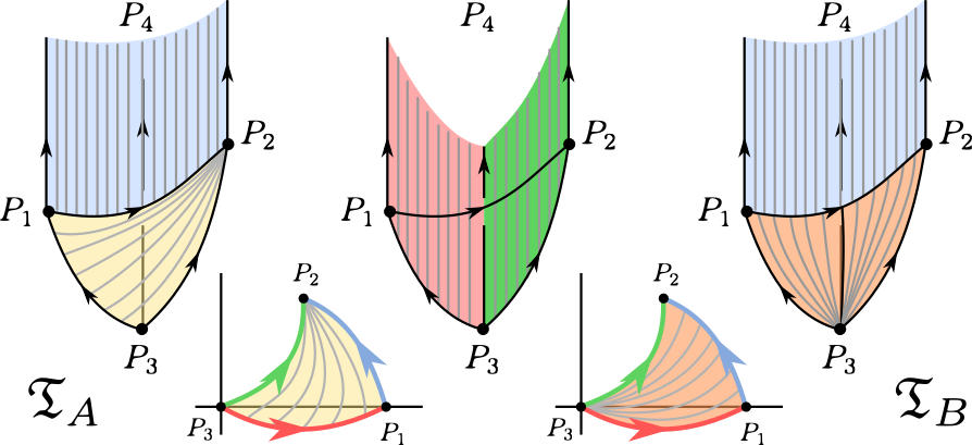 Figure 1
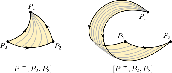 Figure 2
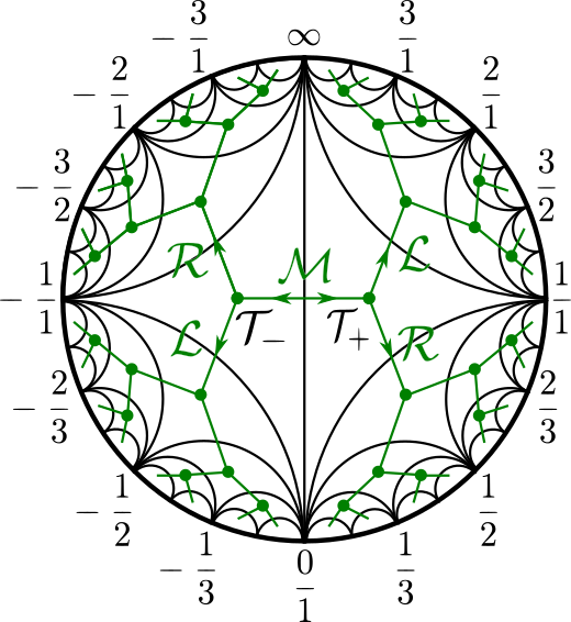 Figure 3
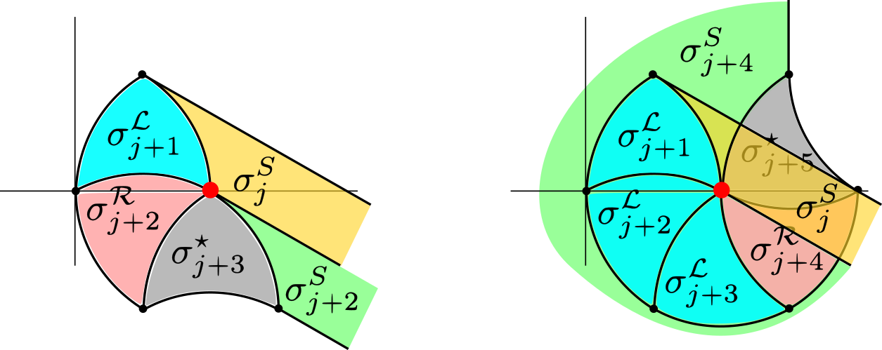 Figure 4
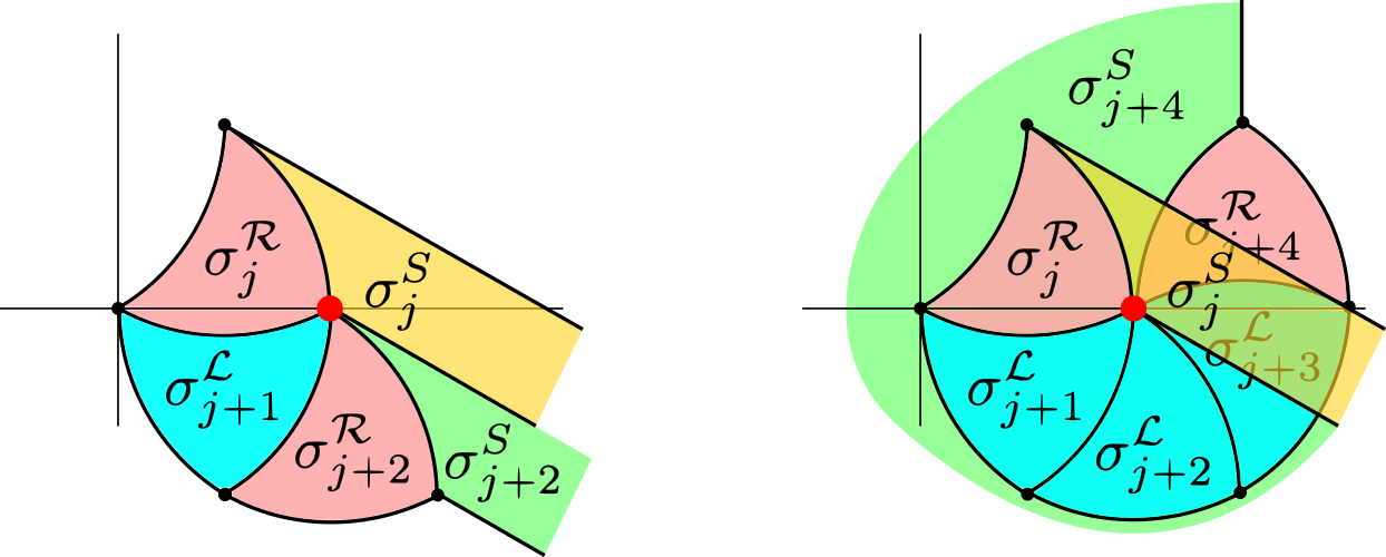 Figure 5
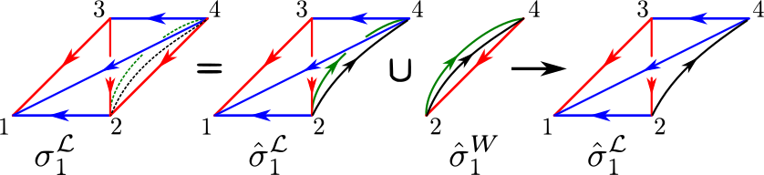 Figure 6
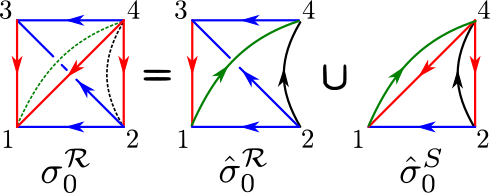 Figure 7
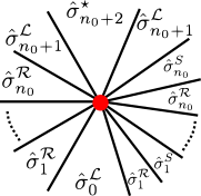 Figure 8
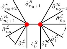 Figure 9
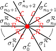 Figure 10
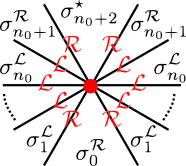 Figure 11
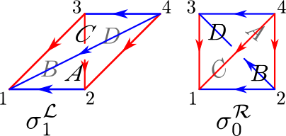 Figure 12
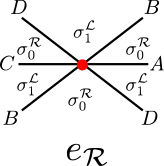 Figure 13
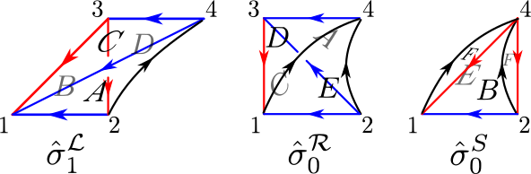 Figure 14
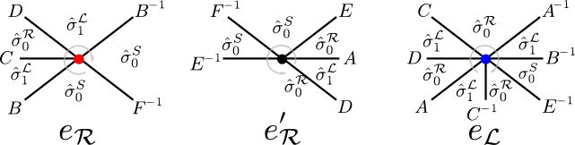 Figure 15
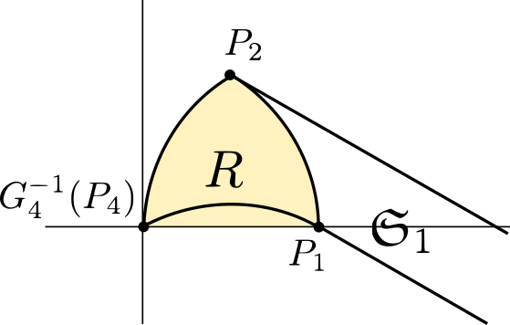 Figure 16
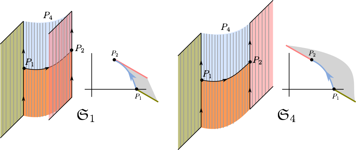 Figure 17
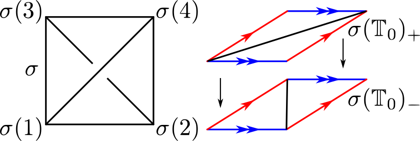 Figure 18
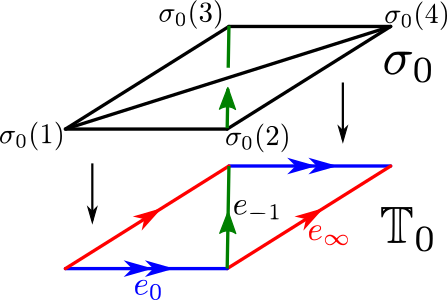 Figure 19
| CR face pairing | –cells | Vertices disjoint from | –coordinates |
|---|---|---|---|
| , | |||
| CR face pairing | –cells | Vertices disjoint from | –coordinates |
|---|---|---|---|
| , | |||
| CR face pairing | –cells | Vertices disjoint from | –coordinates |
|---|---|---|---|
Peer Reviews
No public reviews on file for this paper yet. If you reviewed it on a platform where reviews are public (OpenReview, ICLR, NeurIPS, ICML), you can paste yours below so the community can read it here.
Videos
No videos yet. Explain this paper in a talk, walkthrough, or lecture? Add one.
Taxonomy
TopicsHomotopy and Cohomology in Algebraic Topology · Geometric and Algebraic Topology · Nonlinear Waves and Solitons
Branched Cauchy-Riemann Structures on Once-Punctured
Torus Bundles
Alex Casella
Alex Casella,
Departement of Mathematics,
Florida State University,
FL 32303 USA
https://www.math.fsu.edu/ casella/
Abstract
Unlike in hyperbolic geometry, the monodromy ideal triangulation of a hyperbolic once-punctured torus bundle has no natural geometric realisation in Cauchy-Riemann (CR) space. By introducing a new type of –cell, we construct a different cell decomposition of that is always realisable in CR space. As a consequence, we show that every hyperbolic once-punctured torus bundle admits a branched CR structure, whose branch locus is the set of edges of . Furthermore, we explicitly compute the ramification order around each component of the branch locus and analyse the corresponding holonomy representations.
keywords:
Geometric Structures, Cauchy, Riemann, Torus Bundles, Ideal Triangulations, Branching
\primaryclass
57M50; 32V05
1 Introduction
A geometry or geometric structure is a homogeneous space together with a transitive action on by a Lie group , which acts as the symmetry group of the geometry. This concept was originally introduced by Klein in his celebrated Erlangen program [17], and rapidly developed by Ehresmann [6] and many others afterwards. When and are chosen appropriately, one recovers many classical geometries like hyperbolic , Euclidean or spherical geometry. A –manifold is a manifold endowed with a –structure, namely an atlas of charts in the model space , whose transition functions are restrictions of elements of .
As more and more connections between topology and geometry were discovered, –structures have become a central topic in the study of manifolds. Among many contributors, William Thurston is one of the most celebrated pioneers. In [26], he develops a way to construct hyperbolic structures on cusped –manifolds using ideal triangulations, namely decompositions into tetrahedra whose vertices are removed. The strategy consists in realising these simple pieces as hyperbolic objects, that glue up coherently in the manifold . Consistency of the gluings can be encoded in a system of complex valued equations, whose solutions correspond to hyperbolic structures on . Since Thurston, many authors have studied and further developed his technique ([4], [5], [11], [21], [25], [29], et al.).
In two recent papers ([7], [8]), a similar strategy was employed to construct branched Cauchy-Riemann structures (CR in short) on the complement of the figure eight knot. CR geometry is modelled on the three-sphere , with the contact structure obtained by the intersection , where is the multiplication by in (see for example [2]). The operator restricted to defines the standard CR structure on . Its group of CR automorphisms is , thus a manifold has a (spherical) CR structure when it is endowed with a geometric –structure. The fact that every –manifold admits a contact structure [20] suggests that CR geometry has the potential to play an important role in three dimensional topology. Nevertheless, only few examples of CR manifolds are known. Most of them are closed Seifert fibred manifolds [16] or obtained by Dehn surgery from the Whitehead link [23, 24]. On the other hand, some examples of –manifolds which have no CR structures are known [12].
Inspired by the work of Falbel in [7], we deal with a more general notion of CR structures, by allowing branching. Charts are not diffeomorphisms anymore, but locally branched coverings. By relaxing this condition, one obtains a geometric structure whose developing map is locally injective everywhere except for a nowhere-dense set, the branch locus. The spaces we investigate here are once-punctured torus bundles, orientable manifolds which are the interior of compact –manifolds with boundary a torus. They are fiber bundles over the circle, with fiber space a once-punctured torus. The figure eight knot complement is one such example. Most of these manifolds are hyperbolic [22], and exhibit important combinatorial properties. In particular, Floyd and Hatcher showed that each hyperbolic once-punctured torus bundle admits a canonical realisation as an ideal triangulation, called the monodromy ideal triangulation [10]. This type of triangulation is part of a larger class of fundamental triangulations called veering triangulations, developed by Agol in [1]. The importance of this decomposition relies on its rich combinatorial structure, but also on its geometric properties. For example, Lackenby showed it to be geometrically canonical in the sense of Epstein-Penner [18], while Guéritaud used it to recover Thurston’s hyperbolicity of once-punctured torus bundles [14].
In this paper we modify the monodromy ideal triangulation of each once-punctured torus bundle to a new ideal cell decomposition, that is geometrically realisable in CR space, and whose set of edges constitutes the branch locus. This decomposition is made up of tetrahedra and –cells that we call slabs, CW complexes obtained by deformation retracting the base of a square pyramid onto one of its sides. In the case of the figure eight knot complement, Falbel [7] uses one of these slabs implicitly, as part of a generalised tetrahedron, but the CR structure thus constructed consists of charts that are not embeddings of the tetrahedra. In particular, there is a small neighbourhood of one edge in a tetrahedron that develops to a flat bigon. This is not an obstruction in Falbel’s proof: he focuses on the union of the images of two specific charts and shows that its quotient by the face pairings is homeomorphic to the figure eight knot complement. This strategy is hard to generalise to other punctured torus bundles and it is somehow unnatural. For example, it is true only for the figure eight knot complement that the branch locus occurs precisely at the edges of the triangulation. This suggests the use of a more suitable cell decomposition, such that we can geometrically realise each ideal cell by embedding it in CR space. For this to work, six geometrically different types of slabs will be defined. Each construction is very explicit and calculations are done directly in coordinates in the CR sphere. A collection of the main results is summarised in the following theorem.
Theorem 1**.**
Let be a hyperbolic once-punctured torus bundle. Then admits an ideal cell decomposition that is geometrically realisable in CR space. It corresponds to a branched CR structure, whose branch locus is the set of edges of .
Moreover, the ramification order around each edge only depends on the valence of in , and it is explicitly computable.
The construction presented in this paper has the potential to further extend to more general punctured surface bundles, as they also admit layered triangulations. Although the realisability of the cell decomposition seems to rely on the fact that the base surface is a once-punctured torus, we intend to address this problem in future work using the veering triangulations of Agol [1].
The content of this paper is organised as follows. In sections 2 and 3 we review background material on once-punctured torus bundles and monodromy ideal triangulations. They mostly serve to set notations and underline the most relevant properties. CR geometry is covered in §4. There we define CR tetrahedra and slabs, the two fundamental –cells which will be the building blocks of the CR structures in §5. Section 5 is the core of the paper, where we introduce the notion of branched CR structures and prove Theorem 1, first in the explicit case of the figure eight knot, then in the general case for all once-punctured torus bundles. We conclude by computing ramification orders of the branch locus and a brief analysis of the holonomy representations in §6. In particular, the very last section 6.2 is a summary of some facts about the holonomy representations and the connection to the work of Fock and Goncharov on positive representations [11], mostly for experts.
2 Once-punctured torus bundles
Let be the once-punctured torus endowed with its standard differential structure and standard orientation. The mapping class group of is the group of isotopy classes of orientation preserving diffeomorphisms . For , the once-punctured torus bundle is the differentiable oriented –manifold
[TABLE]
where for . The manifold is a special fiber bundle over the circle, with fiber space , well-defined up to diffeomorphism.
The natural identification of with the square spanned by the standard basis of induces an isomorphism , hence each map has well-defined eigenvalues in (cf. [9]). This characterisation is fundamental to study the geometry of , as for example it helps discerning hyperbolic bundles.
Theorem 2** (Thurston, 1996 [22]).**
* admits a finite volume, complete hyperbolic metric if and only if has two distinct real eigenvalues.*
The element has distinct real eigenvalues if and only if . If the trace is in , then has finite order and is Seifert fibred. While if , then preserves a non-trivial simple closed curve in the punctured torus, which defines an incompressible torus or Klein bottle in . In both cases we get an obstruction to the existence of the hyperbolic metric. An elementary and constructive proof of the other cases can be found in [14].
3 The monodromy ideal triangulation
In this section we recall the canonical realisation of a hyperbolic once-punctured torus bundle as an ideal triangulation, as described by Floyd and Hatcher in [10], called the monodromy ideal triangulation of . For hyperbolic, Theorem 2 implies that the eigenvalues of are distinct with the same sign. To simplify the construction, we are going to make the further assumption that the eigenvalues are positive. This will not cause any loss of generality: if has two negative eigenvalues, then has positive eigenvalues, and the monodromy triangulation of can be easily deduced from the monodromy triangulation of . See Remark 4 for more details.
3.1 Flip sequence
An ideal triangulation of is a maximal collection of pairwise disjoint and non-homotopic (relative the puncture) essential arcs. Every ideal triangulation of comprises three essential arcs, called ideal edges, and divides the surface into two ideal triangles. All of these ideal triangulations are combinatorially equivalent, but they can be distinguished by that they are not isotopic via an isotopy fixing the puncture.
Without loss of generality, one can assume that ideal triangulations of are straight, in the sense that each ideal edge is the intersection with of the quotient of a straight line through the origin in . In a straight triangulation , the slope of an edge is the slope of the corresponding straight line. Since edges start and terminate at the puncture, their slopes must be rational, hence there is a bijection between ideal edges and .
The set of isotopy classes of ideal triangulations can be encoded as the vertices of the Farey tree . This tree is dual to the Farey tessellation (cf. Figure 1), a tessellation of the hyperbolic plane by ideal triangles. The ideal vertices of this tessellation are the set of slopes of ideal edges in the circle at infinity. In particular, the ideal vertices of a triangle in correspond to the slopes of three disjoint non-homotopic properly embedded arcs in , and hence to an ideal triangulation. Thus, there is one vertex of the dual tree for each isotopy class of ideal triangulation of the once-punctured torus, and every such ideal triangulation is uniquely determined by a triplet of slopes satisfying the Farey sum. A beautiful treatment of this topic can be found in [3].
By adopting the convention that [math] and are neither negative nor positive, we say that an ideal triangulation is positive (resp. negative) if at least one if its slopes is positive (resp. negative). The standard positive (resp. negative) ideal triangulation of is the triangulation (resp. ) with slopes (resp. ).
Two vertices of the dual tree are joined by an edge if and only if their corresponding ideal triangulations differ by a single slope. Passing from one triangulation to the other is usually called edge flipping, as it involves removing one edge, resulting in a square with side identifications, and then inserting the other diagonal of the square. As is a tree, every two ideal triangulations of differ by a unique minimal sequence of edge flips.
Edge flips are of three types, depending on the slope we are flipping over. A right flip (resp. left flip ) is an edge flip of the largest (resp. smallest) slope. The remaining flip will be referred to as a middle flip . For example, starting from the standard positive triangulation of , a right flip produces the triangulation , a left flip gives , and a middle flip gives .
One can visualise the dynamics of edge flips on the dual tree as follows. Let be a positive ideal triangulation (different from the standard one) and let be the sequence of triangulations along the unique shortest path between the standard positive triangulation and . By definition, a middle flip kills the middle slope, hence it corresponds to a back-track towards and transforms into , contradicting the minimality of the path. If you exclude back-tracking, one can move along in only two other ways, corresponding to a right or left flip. By orienting the hyperbolic plane with its standard positive orientation, a right (resp. left) flip corresponds exactly to turning right (resp. left) at (cf. Figure 1). A perfectly analogous arguments works if we replace with a negative ideal triangulation.
The following lemma is a direct consequence of the above discussion.
Lemma 3**.**
Let be a positive (resp. negative) ideal triangulation different from the positive (resp. negative) standard one . The unique sequence of edge flips from to does not contain any middle flips. Conversely, the sequence of flips from to only contains middle flips.
Let be a diffeomorphism of the once-punctured torus. The map acts transitively on the set of ideal triangulations of , inducting an isomorphism of the Farey tree . Every isomorphism of a simplicial tree has either a fixed point, or leaves invariant a unique copy of , called axis. The former case happens when and the action is periodic. In the latter case, let be a vertex on the axis. The unique shortest path in from to runs along the axis, and naturally corresponds to a sequence of edge flips. When , the axis has a unique endpoint on the boundary of the hyperbolic plane, and the action is parabolic. Finally we observe that acts on as , hence we will only consider automorphisms with distinct positive real eigenvalues.
After conjugating , one can assume that corresponds to the standard positive ideal triangulation and the axis does not run through any negative triangulation. It follows from Lemma 3 that differs from by a unique sequence of right and left flips. Furthermore, when the eigenvalues of are distinct, always contains at least one right flip and one left flip. In other words, there exist and such that
[TABLE]
We say that is the flip sequence of or of . Its length is the total number of edge flips, namely . Under the canonical isomorphism , a right flip and a left flip correspond to the matrices
[TABLE]
3.2 The triangulation
The following description of the monodromy ideal triangulation is adapted from [14].
The standard ideal tetrahedron is, topologically, a compact tetrahedron with its vertices removed. One can picture as a square with its two diagonals, as in Figure 2. Oriented simplices of are determined by an ordering of the vertices, hence we refer to them by the notation . Sometimes we use the same notation for the unoriented counterparts, but only when it is clear from the context that we ignore the orientation. By identifying the pair of opposite edges and , the exterior of becomes the union of two pleated surfaces, homeomorphic to the once-punctured torus . The top pleated surface is made up of the two ideal triangles , while the bottom pleated surface is made up of the two ideal triangles . Thus the ideal triangulation of is obtained from by an edge flip along .
Suppose is endowed with some ideal triangulation . We say that the tetrahedron layers on if the bottom pleated surface of is glued to via an orientation-preserving combinatorial isomorphism, called the layering. Let be an oriented edge of . We say that layers on along if the chosen layering identifies with the edge . In general, there are six possible ways to layer on , one for each oriented edge of . To simplify the notation we make a further distinction. We say that a layering of is a (right) layering (resp. (left) layering) if layers along the edge with largest (resp. smallest) slope, oriented towards (resp. away from) the origin in . The motivation behind this notation is clear: if right layers (resp. left layers) on , the ideal triangulations of is obtained from by a right flip (resp. left flip).
Let be an element of with two distinct positive real eigenvalues and let be the flip sequence of . Suppose has length . Now we describe how to construct the monodromy triangulation of the hyperbolic once-punctured torus bundle . Suppose is endowed with its negative standard ideal triangulation . Let be a copy of the standard ideal tetrahedron layered on along the edge of slope , oriented as in Figure 3. Then the top pleated surface is triangulated as the positive standard ideal triangulation . For each letter in , , reading from left to right, we perform an layering of a copy of the standard ideal tetrahedron on . The space obtained by stacking these tetrahedra is naturally homeomorphic to . The last top pleated surface is . Its triangulation is obtained from by performing the sequence of edge flips . It follows that , and induces an identification between and which makes into . The monodromy triangulation of is the ideal triangulation consisting of the tetrahedra and the face pairings inherited from the layering construction. As an example, see the monodromy ideal triangulation of the figure eight knot complement in §5.2.
Remark 4**.**
We remark that and act in the same way on the Farey tree, hence they share the same flip sequence. It follows that the monodromy triangulation of differs from the one of only in the way and are identified. More precisely, one can construct by composing the identification between and with a rotation by the angle .
The layering construction induces a natural cyclic ordering of the tetrahedra, thus they will often be indexed modulo . Similarly, one should think of the flip sequence as a cyclic word, with a preferred starting point. For future reference, we introduce the following notation. A tetrahedron of the monodromy triangulation is said to be of type (resp. type ) if the next tetrahedron is layered on top of it by a right (resp. left) layering. We will sometimes record the type of by writing or .
3.3 Combinatorics around the edges
Let be the monodromy ideal triangulation of the once-punctured torus bundle , and let be the length of its flip sequence . Then is made up of tetrahedra , glued together by the layering construction. We denote by the natural quotient map , defined by the face pairings. The space is the interior of a compact –manifold with torus boundary, so its Euler characteristic is zero. It follows that has as many edges as tetrahedra, namely . Nevertheless, each edge may be represented by multiple edges in each tetrahedron. The valence of an edge is the size of its inverse image under .
We are now going to describe the local structure of the edges in . This will be useful in the analysis of the geometry around the edges in §5. We recall that each tetrahedron is a copy of the standard ideal tetrahedron via a canonical identification, hence it inherits labels at the vertices from .
Consider the edge of , and let in . Suppose that is of type . Let , , be the (possibly empty) sequence of tetrahedra of type layered on top of , such that is of type . This sequence corresponds to a subsequence in the word (thought of as a cyclic word). By definition, left layers on , thus . For every , the simplex right layers on , therefore . Finally, left layers on , closing up the sequence of tetrahedra around with the edge . Locally around , the tetrahedra glue to form a ribbon, where and appear once, while every other tetrahedron appears twice. See Figure 4 for a cross section of a neighbourhood of . The simplex (resp. ) is the bottom (resp. top) of the ribbon, and every other simplex constitutes a loop on each side. We deduce that the valence of is .
An analogous picture arises when we assume that is of type , with the difference that every tetrahedron of type is now of type , and vice versa (cf. Figure 5). Furthermore, one may replace with any other tetrahedron in and make the same definitions. For future reference, we summarise all of the above in the following Lemma.
Lemma 5**.**
Every edge in corresponds to a unique subsequence or in , , and a unique ribbon of tetrahedra . The simplex is the bottom of the ribbon, while is the top of the ribbon, and every other tetrahedron in between constitutes a loop on each side. Hence the valence of is .
We remark that uniqueness of the ribbon follows from the fact that the bottom of the ribbon is the only tetrahedron in whose edge is a representative of . Similarly, the top of the ribbon is the only tetrahedron whose edge belongs to . A simple counting argument shows that there is a bijection between the set of tetrahedra and the set of edges, thus associating every edge to its unique ribbon.
4 CR Geometry
The spherical Cauchy-Riemann geometry is modelled on the CR sphere, namely the three-sphere equipped with a natural action. Unlike what we mentioned in the introduction, here we work with a definition of CR space that does not explicitly make use of contact geometry, but it underlines more clearly the action of . This point of view is going to be more suitable and relevant to our context. More details on the connection between CR geometry and contact geometry can be found in [2]. For more background material and proofs of the following Lemmas we refer the reader to § [13] or § [15].
The matrix group preserves the following Hermitian form defined on the complex space :
[TABLE]
Let be the canonical projection, and consider the following cones in ,
[TABLE]
Then is the Siegel domain model of the complex hyperbolic plane and its boundary is
[TABLE]
As a topological space, is homeomorphic to the three-sphere It is the spherical model of the CR sphere. The projective group is the group of its biholomorphic transformations. The action of on is by CR transformations.
We are now going to describe a model for which is particularly suitable for our framework. The Heisenberg group is the space , equipped with the group law
[TABLE]
In the formula above, is the imaginary part of the complex number . Using stereographic projection , one can identify with the one-point compactification of , thus obtaining the Heisenberg model of the CR sphere. In coordinates,
[TABLE]
The action of on is by defined by conjugating with .
Complex geodesics in are totally geodesic submanifolds of real dimension two. Their boundaries in are topological circles, called –circles. A –circles in is the image under of a –circles in .
Lemma 6**.**
In the Heisenberg model , –circles are either vertical lines or ellipses whose projections onto the –plane are circles.
We remark that a complex geodesic in is naturally endowed with a positive orientation given by its complex structure, hence every –circle also inherits an orientation.
Lemma 7**.**
CR transformations map –circles to –circles, preserving their orientations.
Given two distinct points in Heisenberg space , there is a unique –circle between them. We say that points of are in general position if no three are contained in the same –circle. The group of CR transformations acts transitively on pairs of distinct points, while generic configurations of triples of points are parametrised by a real number. Given a cyclically ordered triple of points in , its Cartan angle Å is
[TABLE]
Lemma 8**.**
Three points in are not in general position if and only if their Cartan angle is [math]. Moreover, the group is simply transitive on ordered triples of points in general position with the same Cartan angle.
4.1 CR Edges
Given two distinct points , the oriented edge is the segment of the –circle between and , oriented towards . For example, the oriented edge is the segment , oriented towards . Then is the whole –circle through and . A disk bounded by the loop will be referred to as a bigon.
4.2 CR Triangles
Suppose are three points in general position. For each pair, there are two possible oriented edges, for a total of eight choices of –skeletons defining a triangle. As is simply connected, we can always extend the –skeleton of a triangle to an embedded –cell, with boundary defined by that –skeleton. This can be done in many different ways, all equivalent up to isotopy. Inspired by the work of Falbel [7], we define the marked triangles and as foliations of oriented edges (cf. Figure 6):
[TABLE]
By fixing to be at infinity, a marked triangle is half a cylinder with base part of a finite –circle. One of the advantages of using marked triangles is that they are uniquely determined by their vertices. The following result is a direct consequence of Lemma 7.
Lemma 9**.**
Let and be two triples of points of in general position. Suppose there exists such that , for all . Then
[TABLE]
4.3 CR Tetrahedra and Slabs
Given four points of in general position, a choice of a marked triangle for each triple will not always patch up to form the boundary of a –simplex. On one hand, the faces might not be compatible at the edges and have gaps between them. On the other hand, they could intersect away from the edges. One quickly finds that there is not a canonical choice of marked triangles which always works, thus three dimensional simplices need to be checked on a case by case basis.
Here we are going to describe two fundamental –cells, which will be the building blocks of the CR structures in §5. They are subsets of the Heisenberg space, both topologically homeomorphic to the –ball, but equipped with different simplicial structures. These spaces are defined to be especially symmetric, in the sense that several of their faces can be glued pairwise with monotone maps (cf. Lemma 11). That is not always the case for generic triangles, as previously underlined in Lemma 8.
The standard symmetric tetrahedron. Let be the cube root of unity . We consider the following –tuple of points in general position in Heisenberg space:
[TABLE]
For each triple of points, we consider the following marked triangles:
: the oriented segment is the shortest arc of the circle , oriented from to . The triangle is part of a cylinder, foliated by vertical segments above . 2. 2.
: the edge is an arc of ellipse which projects onto the –coordinate of the Heisenberg space as an arc of the unit circle with centre . It is given by the parametrisation
[TABLE]
Hence is foliated by the vertical rays from to . 3. 3.
: this marked triangle is obtained by a clockwise rotation of the previous triangle . 4. 4.
and : the first marked triangle is foliated by oriented edges from to . For , we have
[TABLE]
where and . The latter one instead, is foliated by oriented edges from to . It can be parametrised as
[TABLE]
Lemma 10**.**
*([7])
The spaces*
[TABLE]
are combinatorially isomorphic to a –simplex. In particular, they bound a –ball on each side in .
The standard (symmetric) tetrahedron of type is the closure of the –ball bounded by the –simplex in (1), which is contained in the upper half of . Similarly, the –simplex in (2) is the boundary of the standard (symmetric) tetrahedron of type . Figure 7 shows and in the Heisenberg model.
These tetrahedra exhibit various symmetries, for example an anti-holomorphic involution swapping the vertices with , and with (cf. [28]). Furthermore, the vertices of each face (taken with the correct cyclic order) have the same Cartan angle,
[TABLE]
As a consequence of Lemma 8 and Lemma 9, we can glue faces of and pairwise by (unique) CR transformations. Consider the following matrices of ,
[TABLE]
These are the unique CR transformations mapping:
[TABLE]
We remark that and are face pairings between two standard tetrahedra of any types, while necessarily glues onto a face of the standard tetrahedron of type . Furthermore, and can be described quite nicely in Heisenberg coordinates:
[TABLE]
The transformation preserves vertical –circles and it restricts on the –plane to a clockwise rotation around the point . The transformation is a anticlockwise rotation of around the vertical –circle through .
The slabs. The next fundamental piece that we are going to define is of the combinatorial type of the CW complex obtained by deformation retracting the base of a square pyramid onto one of its sides. In particular, it is a –cell bounded by two triangular faces and two bigons. It contains a total of five –cells and three [math]–cells.
We define the following bigons of :
[TABLE]
We remark that both and are foliated by vertical –circles. In particular, for all . Moreover,
[TABLE]
The CW complex obtained by attaching
[TABLE]
is topologically a –sphere. For all , it bounds a –ball containing the point . We define the slab to be the closure of such –ball. The slabs and are geometrically equivalent if and only if , in the sense that there is such that . This is due to the fact that the –skeletons of and only differ along one face. Whence we defined a total of six different slabs. Two examples and are depicted in Figure 8.
As we mentioned earlier, , hence let be the (unique) element of :
[TABLE]
[TABLE]
For all , the CR transformation is a face pairing between the slab and the standard tetrahedron of type .
The use of six different slabs turns out to be necessary in the general construction of §5.3. The reason for the number six is due to the fact that the CR transformations and are all of order six. The connection between them and the slabs is revealed in Theorem 17.
We conclude this section with a definition and an observation. Let and be two CW complexes embedded in , and let be a face pairing between the faces and . Then and might intersect away from . We say that the face pairing is monotone if there are neighbourhoods of in respectively such that . The following result generalises an observation by Falbel [7].
Lemma 11**.**
The transformations are monotone face pairings of the standard symmetric tetrahedra and , while is a monotone face pairing between the slab and the standard tetrahedron of type .
Proof.
The transformations and are simple to check. They preserve vertical –circles, therefore one only needs to check the intersection of the projections of the tetrahedra on the –plane.
On the other hand, and are more tedious. We give a summary of the argument for , and refer to [7] for . Consider the slab and the tetrahedron . The transformation glues to along the face . The remaining vertex of is mapped to the point in Heisenberg space. The projection of the –skeleton of is displayed next to the projection of in Figure 9.
Let be the region of –plane bounded by the straight segment from [math] to , and the projections of the edges and . Then is completely contained in the vertical cylinder of Heisenberg space with base . In particular, there is a neighbourhood of the common face where and only intersect along the face, and therefore is a monotone face pairing between and . By symmetry of the definition, we conclude that is also monotone. ∎
5 Branched CR structures on once-punctured torus bundles
Let be a hyperbolic once-punctured torus bundle. In this section we prove the main result of this paper, that admits a branched CR structure (cf. Theorem 17). We start by formalising the notion of a branched CR structure on . Definitions and terminology are inspired by the work on branched analytic structures on Riemann surfaces in [19]. Then we describe CR structures as finite geometric realisations of ideal decompositions. Finally, we give the construction for the figure eight knot §5.2 and in the general case §5.3.
A branched covering between two manifolds is a covering map everywhere except for a nowhere-dense set, called the branch locus. For example, the standard CR branching map defined by is a branched map of ramification order . In particular, is locally injective everywhere except at the branch locus, namely the Heisenberg –axis, where the total angle is .
A CR branched coordinate covering of consists of an open covering of together with branched coverings into open subsets of the CR space , that are locally modelled on the standard CR branching map . A branched CR cover is a coordinate covering such that, on each non-empty intersection , there are homeomorphisms called coordinate transition functions
[TABLE]
that are restrictions of elements in . In particular they satisfy . A branched CR structure on is an equivalence class of branched CR covers, where two branched CR covers are equivalent if their union is a branched CR cover. As a brief example of a natural branched structure, we mention the hypersurface defined by
[TABLE]
We observe that the map defined by is a branched covering, branched along the curve .
Let be a branched CR structure on . When the ramification order of each chart is one, they are homeomorphisms and one recovers the usual definitions of coordinate covering, CR cover and CR structure [26]. We recall that every CR structure admits a developing map and a holonomy representation,
[TABLE]
such that
[TABLE]
The developing map is considered up to deck transformation invariant isotopy, and the pair is uniquely determined up to the following action of :
[TABLE]
Developing maps thus obtained are locally injective, as the charts are homeomorphisms. Vice versa, a locally injective developing map together with a holonomy representation satisfying the equivariancy condition (3), always defines a CR structure. We refer the reader to [27] for a full treatment in the wider context of geometric –structures.
In a similar fashion, one may construct developing maps and holonomy representations for branched CR structures. From the motivational point of view, given only a representation into , it is not clear that it occurs as the holonomy representation of a spherical CR structure. In that sense, it is useful to consider the more general definition of a branched structure, in the hope that any given representation might be understood in a geometric way. The only difference being that developing maps are not locally injective but locally branched coverings. In particular, the holonomy around each connected component of the branch locus is a rotation by an integer multiple of , and therefore trivial, ensuring a well defined representation of .
5.1 Finite geometric realisations
In §5.3 we construct special branched CR structures on , whose branch locus is a disjoint union of curves. The strategy is to use an ideal cell decomposition of , modelled on its monodromy ideal triangulation , whose edge set is the branch locus. We are going to realise each ideal cell as a geometric object in Heisenberg space and each face pairing as an element of , in a compatible fashion. More precisely, suppose is made up of the ideal –cells , with face pairings . We recall that a face pairing is called monotone when the paired cells only intersect along the common face in a neighbourhood of such face (cf. end of §4.3). A geometric realisation of in consists of embeddings and CR transformations , satisfying the following condition: if is the gluing map between the faces and of the ideal –cells and respectively, then is a monotone CR transformation pairing and in the same combinatorial way. Then we say that and are geometric realisations of and respectively.
A geometric realisation differs from a branched CR structure only at the edges. For each edge , consider a small oriented loop around , with prescribed starting point contained in the interior of some cell. Let be the sequence of faces in containing , ordered as they are crossed by , starting from . As travels through a face , it leaves an ideal cell to enter another ideal cell (possibly equal to ). Let be the face pairing gluing to along , and let be its corresponding geometric realisation. Then the geometric holonomy of along is the product . We remark that a different choice of only changes the geometric holonomy by conjugation or by inverse, hence whether the geometric holonomy around an edge is trivial (namely equal to the identity) or not, does not depend on the choice of .
In general, it is not guaranteed that the geometric holonomy is trivial because a geometric realisation does not enforce any conditions on the local structure around the edges. However, when that is the case for every edge of the cell decomposition, then a geometric realisation can be extended to a branched CR structure. More precisely, there is a branched CR structure on whose set of charts include the embeddings , and the coordinate transition functions along the faces are the CR transformations . In particular, it is important that the maps are monotone to ensure local injectivity at the faces. Furthermore, the fact that the geometric holonomy around an edge is trivial allows the construction of a chart containing which is a branched covering (with branch locus ) and which agrees with around . An example of this construction can be found in [29], in the particular case of triangulations and hyperbolic structures.
For future reference, we summarise the above discussion in the following result.
Lemma 12**.**
Let be a geometric realisation of in . If the geometric holonomy around each edge is trivial, then defines a branched CR structure on .
In a similar fashion to ideal triangulations, the ideal cell decomposition we are going to construct is the complement of the [math]–skeleton of a CW complex, which is also called . This CW complex is topologically homeomorphic to the end-compactification of . It has a single vertex, which is the only non-manifold point. When talking about (ideal) cells in , it will be convenient to consider the [math]–skeleton as a point of reference, but we will not always underline that it is not actually part of the decomposition of . Moreover, we are often going to drop the word “ideal” when it is clear from the context.
A finite geometric realisation of in is a geometric realisation whose embeddings extend to the [math]–skeleton. Finite geometric realisations are slightly easier to deal with, as we can use the image of the [math]–skeleton as reference points for the cells. Let be the ideal cell decomposition of the universal cover induced by . If is a finite geometric realisation with trivial geometric holonomy around each edge, then it defines a branched CR structure, represented by some pair of developing map and holonomy representation. By finiteness, the developing map extends equivariantly to the [math]–skeleton . More precisely, if is the restriction of to , then
[TABLE]
5.2 The figure eight knot complement
The figure eight knot complement is the –manifolds obtained by removing a closed tubular neighbourhood of the figure eight knot from the three-sphere. Topologically, it is homeomorphic to the once-punctured torus bundle associated to the flip sequence . The corresponding monodromy ideal triangulation has two tetrahedra: of type and of type (see Figure 10). As a cyclic word, has a subsequence and a subsequence , corresponding to the two edges and of respectively (cf. Lemma 5). Both edges have valence six. The ribbon of tetrahedra around is , as depicted in Figure 11.
Now we construct a branched CR structure on , as a preliminary example for the general case in §5.3. The structure we are going to describe here was first discovered by Falbel [7].
Let be the cell decomposition obtained from the following manipulations on the triangulation .
- (1)
(Figure 12) We subdivide the face of the tetrahedron into two –cells, by introducing a –cell with endpoints . The two –cells thus obtained are combinatorially a triangle and a bigon. Similarly, we subdivide by placing a –cell with endpoints . Finally, we split the tetrahedron into two –cells, by introducing a triangular –cell with endpoints . Whence is subdivided into two –cells: with vertices is combinatorially isomorphic to a simplex, and with vertices is of the combinatorial type of a slab (cf. §4.3). 2. (2)
(Figure 13) Similar to above, we subdivide into two –cells by introducing a –cell inside the tetrahedron bounded by two –cells with endpoints . They are embedded in the faces and respectively. Thus is decomposed into two –cells . The former, has four triangular faces and a bigon. The latter is of the combinatorial type of a wedge, the CW complex obtained by quotienting a face of a –simplex to a point. Its set of vertices is . 3. (3)
(Figure 13) We deformation retract the wedge onto the bigonal face bounded by the red and the black edge. Simultaneously, we collapse the bigonal face of into the black edge, transforming back into a –simplex. Finally, we remove the retracted wedge from the decomposition. As a consequence, the green edge and the black edge of are now identified (cf. Figure 12 and Figure 14).
A few remarks are in order. Up to step (2), the subdivisions of and agree along the faces, hence they form a well defined cell decomposition of . The importance of this step relies on the fact that the new cell decomposition has more edges than , hence a larger set where we can possibly branch on. On step (3), we flatten the –cell and remove it. This does not change the topology of the complex because a neighbourhood of the red edge contains other –cells other than . In the end we have three –cells , two of which are of the combinatorial type of a tetrahedron and one of which is a slab (see Figure 14). They glue to form a CW complex , which is a cell decomposition of . Step (3) is crucial because, by removing the wedge from the decomposition, we avoid the problem of having to geometrically realise it in CR space by an embedding. We remark that in [7], Falbel develops this wedge into a flat bigon.
The slab has two bigonal faces, with endpoints and . Since it would be ambiguous to refer to the edges of by their vertices, we fix the convention that and are the edges belonging to the face shared with , while and are the others. We will say more about these choices below.
We consider the following finite geometric realisation of in . Let and be the two standard symmetric tetrahedra and the slab defined in §4.3. The geometric realisations of the ideal cells are the combinatorial isomorphisms defined by
[TABLE]
We remark that maps the edges and to the segments of –circles going from and , respectively, to . Similarly, and are mapped to the segments of –circles going from to and , respectively.
The geometric realisations of the face pairings depicted in Figure 14 are the matrices defined in §4.3, the identity matrix and a combination thereof. More precisely,
[TABLE]
The product , namely the geometric realisation of , maps the bigonal face of to its other bigonal face . The combinatorics of around the red , black and blue edges are displayed in Figure 15. One computes that the geometric holonomies are trivial:
[TABLE]
[TABLE]
As per Lemma 12, this finite geometric realisation of in corresponds to a branched CR structure on . By developing the cells in , one finds that the order of the branching around the edges and is one, while it is two around . These ramification orders were stated incorrectly in [7], and corrected later in [8, Remark 6.1].
5.3 General case
Now we focus on the general case, to show that every hyperbolic once-punctured torus bundle admits a branched CR structure. In particular, we construct an ideal cell decomposition of , and a finite geometric realisation of it in , with trivial geometric holonomy around each edge.
The ideal cell decomposition. Let be an automorphism of the once punctured torus with two distinct positive real eigenvalues, and let be the corresponding hyperbolic once-punctured torus bundle. Suppose the flip sequence of has length . Then the monodromy ideal triangulation of is made up of ideal tetrahedra . The ideal cell decomposition of is obtained from by performing the three manipulations described in §5.2 to each tetrahedron. We recall from §3.2 that a tetrahedron is said to be of type (resp. type ) if the next tetrahedron is layered by a right (resp. left) layering. Thus we modify every tetrahedron of type as in step (1), and every tetrahedron of type as in (2) and (3). We provide a synthesis of those operations to refresh the notation.
- (1)
Every tetrahedron of type is subdivided into two –cells, along a newly introduced triangular –cell with vertices . They are a tetrahedron and a slab . 2. (2)
Every tetrahedron of type is decomposed into two –cells . The former has four triangular faces, and a bigon where the wedge glues to. 3. (3)
We deformation retract the wedge onto a bigonal face, then remove it. Simultaneously, we collapse the bigonal face of into one edge, transforming back into a –simplex.
Up to step (2), it is easy to check that the performed subdivisions agree along the faces of , hence they form a well defined cell decomposition of .
Now consider the wedge . We claim that around each of its edges there is always at least one –cell that is not a wedge. This is clear for two of its edges, as it glues to the tetrahedron . Call the remaining edge of . Let be the simplex of from which is obtained, and let be the next tetrahedron that left layers on top of . If is of type , then glues to the wedge around . On the other hand, if is of type , then glues to the slab around . Because has two distinct real eigenvalues, its flip sequence always contains at least one and one (cf. §3.1). It follows that around there is always at least one slab. This ends the proof of the claim.
On step (3), we flatten the wedges and remove them. It is a consequence of the claim that this does not change the topology of the complex. Thus in the end we have a CW complex , consisting of three types of –cells, two of which are of the combinatorial type of a tetrahedron and one of which is a slab. The complement of the [math]–skeleton is an ideal cell decomposition of . We remark that has a more edges than , and they are all going to be (non–trivially) branched (cf. §6.1).
To avoid introducing new terminology, we are going to make the following abuse of notation. Cells of coming from tetrahedra of of type (resp. type ) will also be referred to as cells of type (resp. type ). Moreover, if a tetrahedron right layers (resp. left layers) on a tetrahedron in , then also the –cells of obtained from right layer (resp. left layer) on the cells obtained from .
Combinatorics around the edges. As mentioned in the example of figure eight knot complement, a slab has two bigonal faces, therefore it is ambiguous to refer to its edges by the [math]–skeleton. We avoid that by fixing the convention that and are the edges belonging to the face shared with the tetrahedron , , while and are the others. The notation is motivated by the natural orientations of the edges of a geometric slab .
Recall that is the natural quotient map from the disjoint union of the simplices of into , defined by the face pairings. Let be the corresponding map for . Then the valence of an edge in is the size of its inverse image under .
Theorem 13**.**
Let be the set of –cells in . Let be the subset of indices such that is a slab of . Then the quotient map restricts to a bijection
[TABLE]
Theorem 13 allows us to canonically pick a representative for each edge in . For example, in the case of the figure eight knot complement in §5.2, the chosen representatives are and (respectively the blue, black and red edge in Figure 14). Its proof is a consequence of the following two Lemmas, where we deduce the valence of edges in from their counterparts in .
Lemma 14**.**
Let be a –cell of type in , corresponding to a tetrahedron in . Let be the valence of . Then the equivalence class of in is
[TABLE]
where . In particular has valence .
Proof.
By Lemma 5, the edge corresponds to a unique subsequence of , for . In particular, is the bottom of a unique ribbon of tetrahedra
[TABLE]
where is undetermined. Whence is identified with the edges
[TABLE]
The valence of its equivalence class in is . In , we introduce a slab around each edge , while neighbourhoods of the other edges glued to are unchanged (cf. Figure 16 for ). The statement of the Lemma follows. ∎
Lemma 15**.**
Let and be –cells of type in , corresponding to a tetrahedron in . Let be the valence of . Then the equivalence class of in is
[TABLE]
Similarly, the equivalence class of in is
[TABLE]
In particular, both and have valence .
Proof.
As in the proof of Lemma 14, the edge corresponds to a unique subsequence in , for . The ribbon of tetrahedra around its edge class in is
[TABLE]
In particular is glued to the edges
[TABLE]
In , the cell splits into the bigon with boundary and . The two loops of the ribbon of tetrahedra around are split and equidistributed around those two edges (cf. Figure 17 for ). The statement of the Lemma follows. ∎
Proof of Theorem 13.
First we notice that is well defined, as it is the restriction of the natural quotient map . Injectivity follows from Lemma 14 and Lemma 15, because the equivalence classes of and are distinct.
By a topological argument, we deduce that the Euler characteristic of is zero. Therefore has as many –cells as –cells. It follows that is an injective map between finite sets with the same sizes, thus it is a bijection. ∎
The finite geometric realisation in . A finite geometric realisation of consists of embeddings of the –cells into , and geometric realisations of the face pairings.
Let be a tetrahedron of , . The development of depends on the tetrahedron it layers on. More precisely, let be the tetrahedron in on top of which layers. Then the geometric realisation of is the combinatorial isomorphism
[TABLE]
Now let be a slab of . Let be the valence of the edge . Then the geometric realisation of is the combinatorial isomorphism
[TABLE]
More precisely, we require that and . Thus the bigon with endpoints is developed into
[TABLE]
while the bigon with endpoints is realised by
[TABLE]
Both and are foliated by vertical –circles.
Most of the geometric realisations of the face pairings are uniquely determined by Lemma 8. They are the CR transformations described in §4.3. The remaining ones are either the identity matrix , or products of the ’s. We describe them in more detail below. Let be a tetrahedron of , of type .
If is the standard symmetric tetrahedron of type , then layers on a tetrahedron of type . In particular they share two pairs of faces. Let for some . Then the geometric realisations of the face pairings between and are:
[TABLE]
Now suppose is the standard symmetric tetrahedron of type . In this case layers on a tetrahedron of type and on a slab . Let , for some , and let . Then the geometric realisations of the face pairings between and are
[TABLE]
These cover all cases, except for the gluing maps between the bigonal faces of the slabs. Contrary to marked triangles, bigons in Heisenberg space can be identified via many CR transformations. Earlier in this section we showed that around each edge in there is at most one face pairing gluing two slabs along their bigons (cf. Lemma 14 and Lemma 15). Whence we are going to geometrically realise those face pairings so that the geometric holonomy around each edge is trivial. Under this condition, the choices turn out to be unique.
Consider the slab . By Lemma 15, the equivalence class of the edge is
[TABLE]
Let be the sequence of geometric realisations of the face pairings around , starting from to , travelling anticlockwise from the point of view of the vertex . So for example realises the face pairing between and , while corresponds to and (cf. Figure 17 on the right). We remark that is geometrically realised by the slab , because the edge has valence .
Lemma 16**.**
The matrix product is a geometric realisation of the face pairing between and . In particular, it identifies the bigon of with the bigon of .
Proof.
By construction, and are the identity matrix. On the other hand, and , for all . Therefore
[TABLE]
We recall from §4.3 that the CR transformations and preserve vertical –circles, and restrict to rotations on the –plane. In particular, maps to the bigon and maps to . The Lemma follows. ∎
We remark that the face pairing is monotone, thus this completes the construction of the finite geometric realisation of . We conclude the section by showing that these geometric realisations are indeed branched CR structures.
Theorem 17**.**
The geometric holonomy around each edge in is trivial and therefore the geometric realisation defines a branched CR structure on .
Proof.
We recall that by Theorem 13 there is a canonical representative for each edge in .
Let be the subset of indexes such that is a slab of , and let be its complement. It is a consequence of Lemma 16 that the geometric holonomy around the edges , for , is trivial.
Consider an edge , for . Let be the sequence of geometric realisations of all the face pairings around , starting from and travelling clockwise from the point of view of the vertex (cf. Figure 17 on the left). Then we have
[TABLE]
Thus the geometric holonomy around is the product . Because the matrices and are of order six, one only needs to check that the product is the identity matrix for . Straight forward computation of the six products gives the result.
An analogous argument works for the edges , . The geometric holonomy around them is of the form . The matrices and are also of order six, hence one only needs to check that the cases . The calculation is straightforward.
We apply Lemma 12 to complete the proof. ∎
6 Properties of the Structures
Consider the branched CR structure on the hyperbolic once-punctured torus bundle described in the previous section 5.3. We conclude by analysing two important features of the structure: the ramification order around each connected component of the branch locus (namely the ideal edges), and the holonomy representation. In §6.1 we show that the ramification order of an edge has a simple description in terms of the valence of in the cell decomposition, and therefore its explicitly computable (cf. Theorem 13). In §6.2 we find the holonomy of the generators of and underline some properties.
6.1 Branch locus
The branch locus of the CR structure of is set of all ideal edges of the associated cell decompositions . Here we show that the ramification order around each curve is related to their valence in the simplicial complex. The strategy will be to develop each curve as a vertical line in Heisenberg space, and analyse the projection onto the –plane of a neighbourhood. This way we can talk about angles of the projections where otherwise it would not be possible. We remind the reader that CR transformations do not preserve angles, therefore the angles we are going to talk about depend on the chosen realisations.
We recall that by Theorem 13 there is a canonical representative for each edge in the cell decomposition , namely and . Let be the ceiling function, which associates to the smallest integer greater than or equal to .
Lemma 18**.**
Let be the valence of in . Then the ramification order around is .
Proof.
First, we observe that the geometric realisation develops the edge into the vertical ray of Heisenberg space going from to . Therefore we can understand the ramification order of by looking at the projections of the tetrahedra around on the –plane of .
Let be the projection of the standard symmetric tetrahedron. It is a triangular region bounded by three arcs of circles (cf. Figure 7). We recall from §5.3 (cf. Figure 17) that the sequence of –cells around in is
[TABLE]
Then projects onto . The next simplex glues to via , therefore its projection is a clockwise rotation of around the origin. After that, we have simplices each of which is glued to the previous one by . Whence each of their projections , for , is a anticlockwise rotation of about the point . Finally, the projections of the geometric realisations of the two slabs rigidly glue to and to fill in the gap. Examples for and are depicted in Figure 18.
Around , the first region contributes with an angle of , while every other region , for , contributes with an angle of . The first slab also adds . This sums up to . The angle of the projection of the last slab around is a non-negative number strictly lower than , therefore the total angle is the next integer multiple of . That is . ∎
Lemma 19**.**
Let be the valence of in . Then the ramification order around is .
Proof.
This proof is similar to the one of Lemma 18, as the geometric realisation develops the edge into the vertical ray from to . The only difference is that we are not going to consider the projections of the entire cells, since they are not as tidy as in the previous case, but only the projections of the vertices. Every –cell around has two vertices at and , and its angle about is strictly between zero and . Therefore knowing the positions of the other vertices gives us an estimate of the total angle around .
The sequence of –cells around in is
[TABLE]
for some . We begin by developing , then glue every other –cell around . The vertices that are not identified with the endpoints of are listed in Table 1. They are all positioned at the vertices of a regular hexagon of edge length .
We draw examples of the projections for and in Figure 19. We remark that these are projections of the vertices and edges, but not of the –skeletons as faces are generally not foliated by vertical rays anymore.
Up to , the total sum of the angles is strictly between and Because the angle of the projection of the last slab around is a non-negative number strictly lower than , the ramification order must be . ∎
Lemma 20**.**
Let be the valence of in . Then the ramification order around is .
Proof.
We follow almost verbatim the proof of Lemma 19.
First we consider the development . This geometric realisation maps the edge into the vertical ray from to . From the point of view of the vertex (cf. Figure 16), starting from and travelling anticlockwise around until , we encounter the –cells
[TABLE]
The vertices of these cells that are not identified with the endpoints of are listed in Table 2.
Similarly, if we travel clockwise around , we have
[TABLE]
The vertices of these cells that are not identified with the endpoints of are summarised in Table 3.
We remark that for all , the -cells and cover a total angle of around . When , the total angle around is exactly of , hence in the general case the ramification order around is . ∎
6.2 The holonomy representation
It was mentioned in §5 that every branched CR structure admits a pair of a developing map and holonomy representation, defined up to the action of . Let be a representative pair associated to the branched CR structure on . Here we summarise few facts about , referring the reader to the author’s PhD thesis for more details and the connection to the work of Fock and Goncharov on positive representations [11].
The fundamental group of is an HNN extension of the fundamental group of the base once–punctured torus , namely the free group in two generators . It has a standard presentation
[TABLE]
where is the automorphism induced by , and is represented by the base circle of the fiber bundle. If has flip sequence (the other case being similar), there is a choice of the class representative such that
[TABLE]
Let be the representation obtained by restricting to . Then does not depend on , namely it is a representation of that always extends to a representation of . It is irreducible, but not strongly irreducible. Moreover, it is not faithful but it has infinite discrete image. In fact, its image is a subgroup of the Eisenstein-Picard modular group , the subgroup of with entries in the set of Eisenstein integers .
The representation was proved to have the above special properties while studying Fock and Goncharov’s parametrisation of , the decorated –character variety of . Using the inclusion map together with its first complex jet, one induces a decoration on , making its conjugacy class an element of . Under this construction, the Fock-Goncharov coordinate of is
[TABLE]
The point and its complex conjugate are the only points in Fock-Goncharov moduli space that are fixed by every Fock-Goncharov edge flip.
Acknowledgements
The material presented here is based on the PhD dissertation of the author, completed at the University of Sydney in . We heartily thank Stephan Tillmann, the author’s PhD supervisor, for introducing him to the topic, the multiple stimulating conversations and unlimited advices. We thank the PhD examiners Jeffrey Danciger, Antonin Guilloux and Joan Porti whose comments helped improve this manuscript. We also thank Sam Ballas and Lorenzo Ruffoni for their useful suggestions on the original draft. Lastly, we acknowledge the support by the Commonwealth of Australia during the author’s PhD.
The reference list from the paper itself. Each links out to its DOI / PubMed record.
- 1[1] Ian Agol. Ideal triangulations of pseudo-Anosov mapping tori. In Topology and geometry in dimension three , volume 560 of Contemp. Math. , pages 1–17. Amer. Math. Soc., Providence, RI, 2011.
- 2[2] John S. Bland. Contact geometry and CR structures on S 3 superscript 𝑆 3 S^{3} . Acta Math. , 172(1):1–49, 1994.
- 3[3] Francis Bonahon. Low-dimensional geometry , volume 49 of Student Mathematical Library . American Mathematical Society, Providence, RI; Institute for Advanced Study (IAS), Princeton, NJ, 2009. From Euclidean surfaces to hyperbolic knots, IAS/Park City Mathematical Subseries.
- 4[4] Alex Casella, Feng Luo, and Stephan Tillmann. Pseudo-developing maps for ideal triangulations II: Positively oriented ideal triangulations of cone-manifolds. Proc. Amer. Math. Soc. , 145(8):3543–3560, 2017.
- 5[5] Jeffrey Danciger. A geometric transition from hyperbolic to anti-de Sitter geometry. Geom. Topol. , 17(5):3077–3134, 2013.
- 6[6] Charles Ehresmann. Sur les espaces localement homogènes. L’ens. Math. , 35(1):317–335, 1936.
- 7[7] Elisha Falbel. A spherical CR structure on the complement of the figure eight knot with discrete holonomy. J. Differential Geom. , 79(1):69–110, 2008.
- 8[8] Elisha Falbel and Jieyan Wang. Branched spherical CR structures on the complement of the figure-eight knot. Michigan Math. J. , 63(3):635–667, 2014.