Expansion of the resolvent in a Feshbach model
Raffaele Carlone, Domenico Finco

TL;DR
This paper extends previous work on Feshbach resonances by deriving a low-energy expansion of the resolvent for a multichannel Hamiltonian in the resonant case, providing deeper insight into the spectral properties at low energies.
Contribution
It introduces a low-energy expansion of the resolvent for a multichannel Hamiltonian with Feshbach resonances, building upon prior results and focusing on the resonant case.
Findings
Derived a low-energy expansion of the resolvent $( ext{H}-k^{2})^{-1}$ as $k o 0$ in the resonant case.
Extended previous results on Feshbach resonances to include the resolvent expansion at low energies.
Provides mathematical tools for analyzing spectral properties near zero energy in multichannel quantum systems.
Abstract
In this paper we extend the results proved in (Carlone, R., Correggi, M., Finco, D., Teta, A.: A model for Feshbach Resonances arXiv:1901.08282 [math-ph]) about Feshbach resonances in a multichannel Hamiltonian , proving a low energy expansion of the resolvent as in the resonant case.
Click any figure to enlarge with its caption.
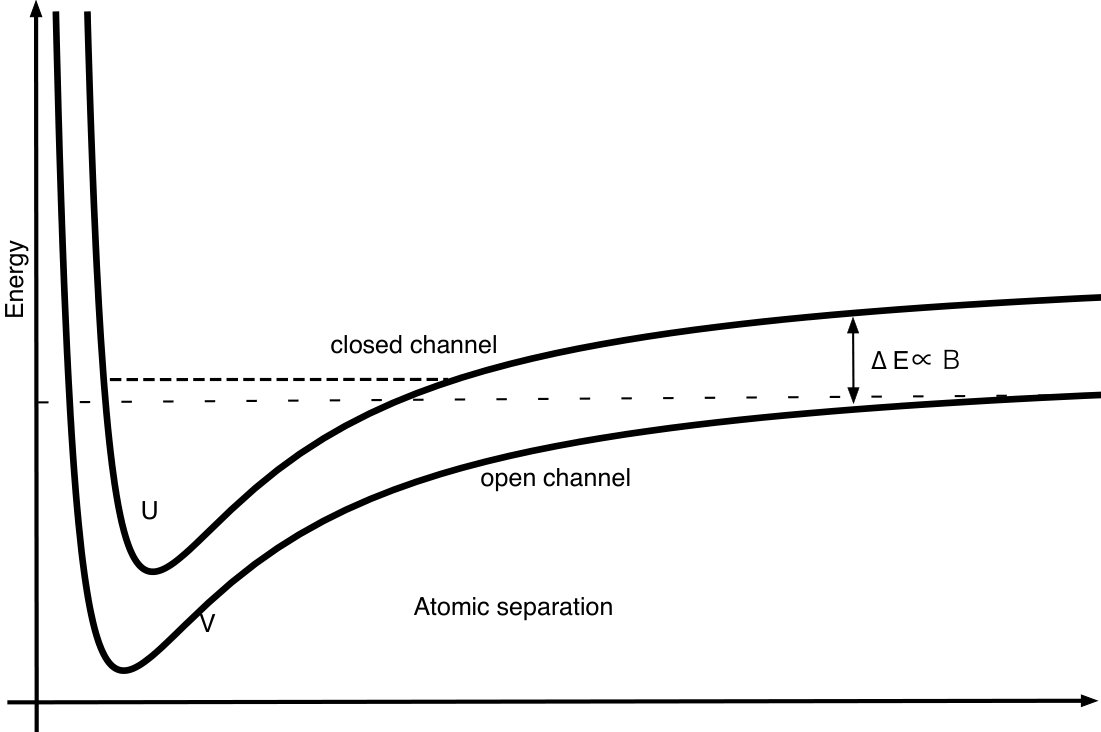 Figure 1
Peer Reviews
No public reviews on file for this paper yet. If you reviewed it on a platform where reviews are public (OpenReview, ICLR, NeurIPS, ICML), you can paste yours below so the community can read it here.
Videos
No videos yet. Explain this paper in a talk, walkthrough, or lecture? Add one.
Taxonomy
TopicsCold Atom Physics and Bose-Einstein Condensates · Quantum, superfluid, helium dynamics · Quantum chaos and dynamical systems
Expansion of the resolvent in a Feshbach model
Raffaele Carlone
Dipartimento di Matematica e Applicazioni “R. Caccioppoli”, Universitá di Napoli “Federico II”, Via Cinthia, Monte S. Angelo, 80126 Napoli, Italy
Domenico Finco
Facoltà di Ingegneria, Università Telematica Internazionale Uninettuno, Corso V. Emanuele II 39, 00186 Roma, Italy
Abstract
In this paper we extend the results proved in ([7]) about Feshbach resonances in a multichannel Hamiltonian , proving a low energy expansion of the resolvent as in the resonant case.
Dedicated to Gianfausto Dell’Antonio on the occasion of his 85th birthday
1 Introduction
The physics of ultracold quantum gases and molecular quantum gases is a research which had had a steep growth in the last twenty years induced by incredible progresses, both from the experimental point of view and from the theoretical one. The wide range of applications covers atomic and molecular physics, condensed matter and few and many-body physics.
A major breakthrough in this field was the experimental observation of a dilute Bose gas condensation in 1995 ([2]) as in the Einstein predictions of 1925 . After this fundamental experimental realization, a big effort was made for a deep understanding of the physical processes involved. A crucial point was to go beyond the mean field physics, to study interactions between ultra cold atoms and observe long and short range correlation phenomena ([18]). The extraordinary degree of control needed on such systems in order to reach these extreme conditions, was really challenging.
From the experimental point of view, besides all the different techniques to control the physical properties of condensate, two of them in particular had greater success: one is the realization of optical lattices of different spatial dimensions ([3],[9]), while the second is the tunability of the scattering length using Feshbach resonances (see [8] and [15] for a review ).
In a dilute quantum gas the density and mobility condition are such that only the two-body scattering processes are relevant. Moreover in many situations, since the typical energies allow only elastic scattering, the most relevant parameter is the scattering length and the possibility to tune it provides an effective mean to control the interaction.
A key feature of Feshbach resonances is the presence of an open channel (where scattering processes are allowed) and a closed channel (where scattering processes are forbidden) with bound states. It may happen that a bound state of the closed channel crosses the ionization threshold of the open channel, that is the bottom of the continuous spectrum of the hamiltonian of the open channel, and strongly interacts deeply influencing the scattering process, see [11], even when the interaction between channel is weak. This is often understood in the physical literature as virtual scattering process with a metastable state at the bottom of the spectrum.
In modern realizations the splitting is realized by applying an external magnetic field to, for instance, alkali atoms and it is due to the coupling of states with different spin quantum numbers with the magnetic field. In this way the energy splitting and energy levels of the bound states of the closed channel can be externally controlled and it is possible to realize the conditions for a Feshbach resonance.
In the physics literature it was obtained a formula relating the scattering length with the magnetic field around the value of the Feshbach resonance ([19])
[TABLE]
where is the scattering length far from the resonant values, is the value of the magnetic field at the resonance and is the resonance width.
The rigorous analysis of resonances has a very long story ([10]): the first mathematical model for multichannel hamiltonian traces back to the original paper of Friedrichs ([12]) in 1948. Many mathematical features of resonances were studied using different strategies, as the dilation-analytic technique ([13]) or simplified models using point interactions ([4],[5],[6]).
Recently in [7] the formation of Feshbach resonances and the dependence of the scattering length from the magnetic field were rigorously studied, proving results about the existence and localization of resonances and the behavior of the scattering length near a resonance.
In section 2, we fix the notation and we recall the main results of [7]. In section 3 we prove a low energy expansion of the resolvent of a matrix hamiltonian when a Feshbach resonance is present; our main result is Theorem 3.5.
2 Existence of Feshbach Resonances
In this section we fix some notational conventions used in the paper and we recall the main results of citeccft.
Bold face letters denote vectors in , e.g., , while scalars are denoted by regular letters, e.g., . When there is no ambiguity we also use the notation for the modulus of a vector .
Since we always deal with functions on , we often omit the base space in Banach space notation, i.e., ; moreover when there is no possible confusion we denote .
We recall the definition of weighted Hilbert spaces: set for short, then, for any , we define
[TABLE]
The closure of w.r.t. the above norm is denoted by . The weighted Sobolev space , , is defined analogously as the closure of w.r.t. the norm
[TABLE]
The conventional Sobolev spaces , can be defined via Fourier transform as the closure of w.r.t. the norms
[TABLE]
where we use the following convention for the Fourier transform
[TABLE]
By the properties of the Fourier transform and a simple exchange of the role of and , one easily gets
[TABLE]
Hence, we obtain the useful identity
[TABLE]
We recall some classical results on spectral and scattering theory mostly taken from [1, 14], which will be used in the proofs. We denote by the Banach space of continuous functions vanishing at infinity equipped with the norm. We also denote by the space of bounded linear operators on and, more in general, stands for the space of continuous linear transformations between two Banach spaces and . Similarly, is the space of compact operators from to and .
Following ([7]) we now make the mathematical setting more precise. We consider a multi-channel scattering of a particle in dimension three: we assume that there are an open channel, where the scattering is energetically possible, and a closed one where any scattering process is forbidden because of an energy constraint (see figure 1).
We describe the system by the following matrix Hamiltonian acting on the Hilbert space :
[TABLE]
[TABLE]
where
[TABLE]
The starting point of our investigation is the eigenvalue equation for the matrix Hamiltonian :
[TABLE]
Writing , where denotes transposition, equation (2.10) is equivalent to the system
[TABLE]
Since we are interested in the low energy behavior, we can restrict to the energies
[TABLE]
For in the resolvent set of , has a bounded inverse in and the system (2.11) is equivalent to the coupled integral equations
[TABLE]
where we have denoted by the generalized eigenfunctions of .The resolvent is defined as a boundary value from the upper half plane. From (2.13) one sees that the problem is reduced to find the solution of the equation
[TABLE]
Definition 2.1** (Ikebe class ).**
We say that a measurable function belongs to the Ikebe class , , if , is locally Hölder continuous except for a finite number of points and there exists and such that
[TABLE]
Assumption 2.2**.**
We assume that
- a)
;
- b)
;
- c)
.
Assumption 2.3**.**
Under this assumptions and are self-adjoint operators on . We assume that
- a)
has negative simple eigenvalues , with corresponding eigenvectors ;
- b)
and zero is neither an eigenvalue nor a resonance;
- c)
in .
We denote by the set of eigenvectors related to positive eigenvalues of , i.e.,
[TABLE]
Proposition 2.4** (Generalized eigenfunctions).**
Let Assumption 2.2 hold true and let be fixed. Then, for any with and , for , equation (2.14) admits a unique continuous solution , such that . Furthermore, satisfies the asymptotics*
[TABLE]
with
[TABLE]
where is the scattering amplitude associated to the potential .
Definition 2.5** (Effective scattering length).**
We define the effective scattering length in the open channel as
[TABLE]
where is given by (2.18)
See [7] for a motivation of this definition.
Theorem 2.6** (Feshbach resonances).**
Let Assumptions 2.2 and 2.3 hold true and let be fixed. Then, there are at least critical values , , with , such that is continuous for and*
[TABLE]
*as , where .
Furthermore, there is such that, if , then the critical values satisfy and any further critical value , with , is such that .*
Corollary 2.7** (Zero-energy equation).**
Under the same assumptions of Theorem 2.6, if , then there exists a distributional solution of the zero-energy equation .*
Clearly the interesting case is when is different from zero. It turns out that this is true if and only if for , we are not in the exceptional case of the second case, according to terminology of Definition 3.4. In other words, we have a Feshbach resonance, if and only if presents a zero-energy resonance; see [7] for details.
3 Low Energy Expansion of the Resolvent
Corollary 2.7 suggests the resolvent is singular as when . In this section we give a characterization of the zero energy eigenspace of and we study some properties of the low energy singularities of the resolvent of . In what follows we will assume always that .
First we recall the Schur-Grushin-Feshbach formula: suppose that , direct sum of linear spaces, and that we have a linear operator on given by
[TABLE]
with invertible. Define . Then exists iff exists and
[TABLE]
We can use formula (3.2) to give a representation of the resolvent of . In this case we put
[TABLE]
It is straightforward to see that exists for . Let then
[TABLE]
and
[TABLE]
We can write for
[TABLE]
then
[TABLE]
For sake of notation we define
[TABLE]
so that
[TABLE]
Notice that, for some . Therefore for ,
[TABLE]
then we have
[TABLE]
In [7], it was proved that if and only there exists such that . Notice that for some and therefore . Indeed if then , , for some some and finally for some some .
Then by Fredholm’s alternative with for , , . Therefore we have for such values of that for if and the boundary value of the resolvent is well defined as an operator between suitable weighted spaces by (3).
We want to discuss the limit of of (3). We have that the existence of is related to the existence of or . For this reason we define
[TABLE]
Both and are finite dimensional for due to the compactness properties pointed out.
Proposition 3.1**.**
The sets and are isomorphic as vector spaces and do not depend on . The linear isomorphisms are given by the restrictions of to and to respectively, that is:
[TABLE]
The operator can be substituted by .
Proof.
Let then , indeed
[TABLE]
The map is injective: if then we have . Moreover it is clear that is the the inverse of on the image of . We prove that is also onto. First notice that on is injective since on . Then if we have and it is sufficient to prove that . This is straightforward since
[TABLE]
This proves that and are isomorphic and (3.10). Since the two spaces have opposite monotony in , they are in facts independent. Notice that and coincides that on by the definition of . ∎
Proposition 3.2**.**
We have and in for .
Proof.
Since then for we have
[TABLE]
Suppose that and . Then by (3.6) and . Hence . ∎
Proposition 3.3**.**
For there exists operators such that
[TABLE]
Proof.
Define as a spectral projection by the analytic functional calculus,
[TABLE]
with sufficiently small that only includes the eigenvalue. This is possible due to the compactness of . Then is invertible and we can define
[TABLE]
Properties (3.11), (3.12) and (3.13) follow from the separation of spectrum, see [16] pg. 178. The operator is finite rank since si compact. Taking into account the identity , we have that has the same regularity of and therefore it is compact. The last property (3.15) can be proved as in Lemma 3.5 in [17]. ∎
Due to Proposition 3.2 and the positivity of by Assumption 2.3, we have that defines a inner product on . At the same time we have that defines an inner product on . Notice that and possess a natural duality induced by inner product since . Under this coupling, if , , is an orthonormal basis in then with is orthonormal in and it is also the dual basis with respect to the above defined inner products. The two bases are orthonormal w.r.t. the two above defined inner products. Moreover the spectral projector reads
[TABLE]
Let us call . It is straightforward to check that if then is a zero-energy eigenvalue of that is and . We can have different cases
Definition 3.4**.**
We say that we are in the generic case if and in the exceptional case otherwise. In the exceptional case we distinguish the following situations: in the first kind and , in the second case and in the third case .
Notice, see [7], that
[TABLE]
Then belongs to iff
[TABLE]
and in particular that is, there is at most one resonance. In the main theorem we discuss the expansion of .
Theorem 3.5** (Low Energy Expansion).**
Let Assumption 2.2 and Assumption 2.3 hold and let be the critical values as in Theorem 2.6. Then if then we are in the generic case and exists. Otherwise if we are in exceptional case and we have the following expansions :*
- •
In the exceptional case of first kind, we have:
[TABLE]
in with and where
[TABLE]
- •
In the exceptional case of second kind assume , then we have:
[TABLE]
in with , , where is the orthogonal projector on the zero-eigenspace of and is defined by (3.32).
We omit the discussion of the exceptional case of the third kind for sake of brevity.
Proof.
The first part of the theorem is just a rephrasing of Theorem 2.6: the critical values are exactly the values of such . Therefore exists by Fredholm’s alternative and with and .
Now we discuss the exceptional case of the first kind. Let us define and decompose accordingly, that is, we put
[TABLE]
Remember that in this case with ; we normalize requiring that . Notice that is continuous and exist by construction. Then exists and it is continuous for sufficiently small by Neumann series. By (3.2) we have to discuss the invertibility of
[TABLE]
on the range of . In facts in this case we have
[TABLE]
The resolvent has the expansion in with and , see Lemma 2.3 in[17] and Lemma 2.3 in [20].
[TABLE]
where ′ denote the derivative w.r.t. . Notice also the analiticity of in in . Then the following expansion in , , holds true:
[TABLE]
Then we have
[TABLE]
where we have put
[TABLE]
Since
[TABLE]
then we have
[TABLE]
The constant is different from 0 otherwise would be a 0-energy eigenstate and we would be in the exceptional case of the second kind. Using again expansion (3.24), we have also and . Therefore we obtain
[TABLE]
Using (3.2) and the above remarks, we see that the only singular terms comes from the term and we obtain
[TABLE]
Then
[TABLE]
and this proves (3.20).
Now we consider the exceptional case of the second case. Again the main point is the inversion of on the range of . In this case we have
[TABLE]
Let us start expanding around
[TABLE]
Taking into account , in the following of the proof we can choose such that . Then the following expansion holds true in with :
[TABLE]
Both (3.29) and (3.30) do not contribute in the expansion of (3.28): the former since and the latter due to (3.25) and the cancellation condition in (3.27) (remember that ). Now we discuss the first term in (3.32): for the same reasons as in the analysis of (3.30) we have
[TABLE]
Notice that in (3.33) we have used Lemma 2.6 of [17] and the cancellation condition in (3.27). For the second term (3.32) we have
[TABLE]
Define the matrix by
[TABLE]
Since is positive definite, we can define and . Then is orthonormal basis of w.r.t. the inner product and
[TABLE]
By the same arguments we have
[TABLE]
Collecting the above results we have
[TABLE]
where we have denoted by the expression in (3.32). Using (3.2) and the above remarks, we see that the only singular terms comes from the term and we obtain
[TABLE]
in . Since wei finally obtain
[TABLE]
in with , . which proves (3.21) ∎
We expect that the hypothesis on the potential are not optimal w.r.t. to the decay at infinity. We have discussed the most simple expansion of the resolvent while leaving untouched the differentiability of the remainder which is a central issue in the proof of dispersive estimates and boundedness properties of the wave operators.
The reference list from the paper itself. Each links out to its DOI / PubMed record.
- 1[1] Agmon, S.: Spectral properties of Schrödinger operators and scattering theory. Ann. Scuola Norm. Sup. Pisa Cl. Sci. 2 (1975).
- 2[2] Anderson, M. H., Ensher, J. R., Matthews, M. R., Wieman, C. E., Cornell, E. A.: Observation of Bose-Einstein condensation in dilute atomic vapor. Science 269 , 198-201 (1995).
- 3[3] Bloch, I.: Ultracold quantum gases in optical lattices. Nature Physics 1 , 23-30 (2005).
- 4[4] Cacciapuoti, C., Carlone, R., Figari, R.: Resonances in models of spin dependent point interactions. J. Phys. A:Math. Theor. 42 , 035202 (2009).
- 5[5] Cacciapuoti, C., Carlone, R., Figari, R.: Perturbations of eigenvalues embedded at threshold: I. One-and three-dimensional solvable models. J. Phys. A:Math. Theor 43 , 474009 (2010).
- 6[6] Cacciapuoti, C., Carlone, R., Figari, R.: Perturbations of eigenvalues embedded at threshold: Two-dimensional solvable models. J. Math. Phys. 52 , 082515 (2011).
- 7[7] Carlone, R., Correggi, M., Finco, D., Teta, A.: A model for Feshbach Resonances, in preparation.
- 8[8] Chin, C., Grimm R., Julienne P., Tie-singa, E.: Feshbach resonances in ultracold gases. Rev. Mod. Phys. 82 , 1225-1286 (2010).