Multi-Dimensional Balanced Graph Partitioning via Projected Gradient Descent
Dmitrii Avdiukhin, Sergey Pupyrev, Grigory Yaroslavtsev

TL;DR
This paper introduces a scalable multi-dimensional balanced graph partitioning method using projected gradient descent, improving distributed graph processing performance on large-scale social networks.
Contribution
It presents a novel scalable algorithm for multi-dimensional balanced graph partitioning based on randomized projected gradient descent for non-convex relaxations.
Findings
Outperforms state-of-the-art methods on large social networks
Efficient implementation of the algorithm in practice
Demonstrates importance of multi-dimensional balance for performance
Abstract
Motivated by performance optimization of large-scale graph processing systems that distribute the graph across multiple machines, we consider the balanced graph partitioning problem. Compared to the previous work, we study the multi-dimensional variant when balance according to multiple weight functions is required. As we demonstrate by experimental evaluation, such multi-dimensional balance is important for achieving performance improvements for typical distributed graph processing workloads. We propose a new scalable technique for the multidimensional balanced graph partitioning problem. The method is based on applying randomized projected gradient descent to a non-convex continuous relaxation of the objective. We show how to implement the new algorithm efficiently in both theory and practice utilizing various approaches for projection. Experiments with large-scale social networks…
Click any figure to enlarge with its caption.
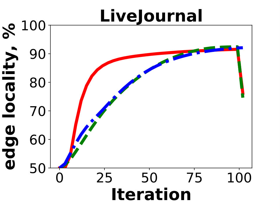 Figure 1
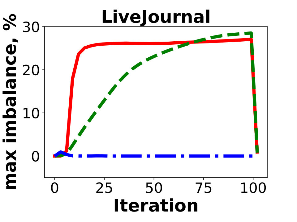 Figure 2
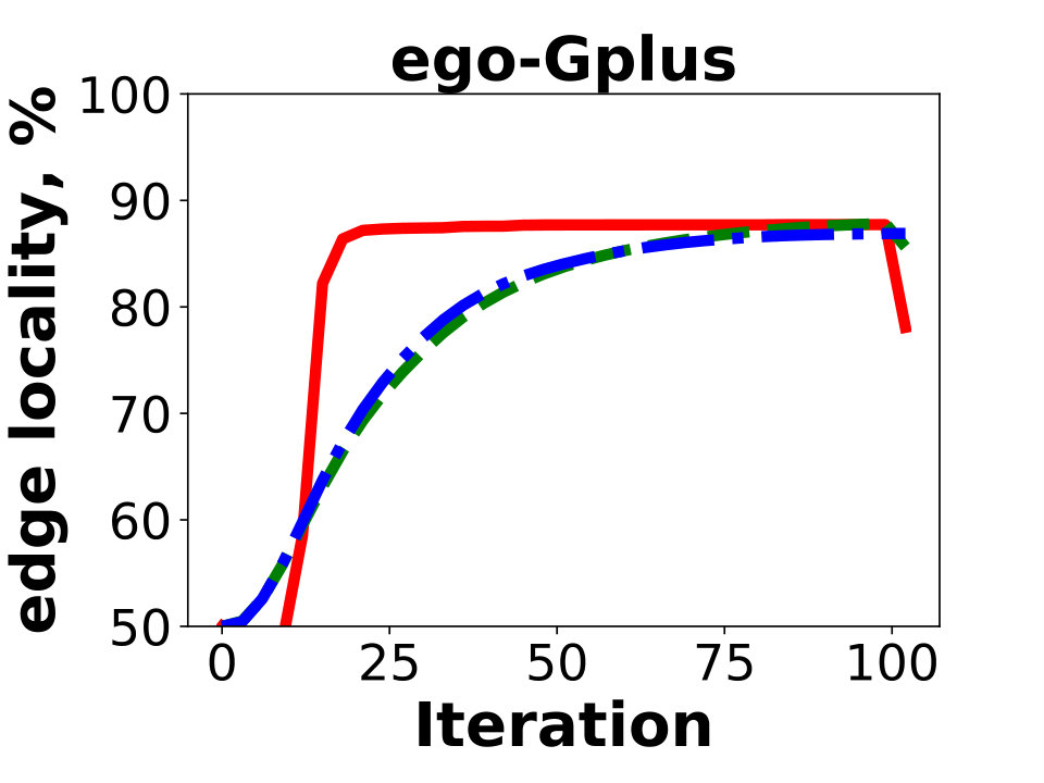 Figure 3
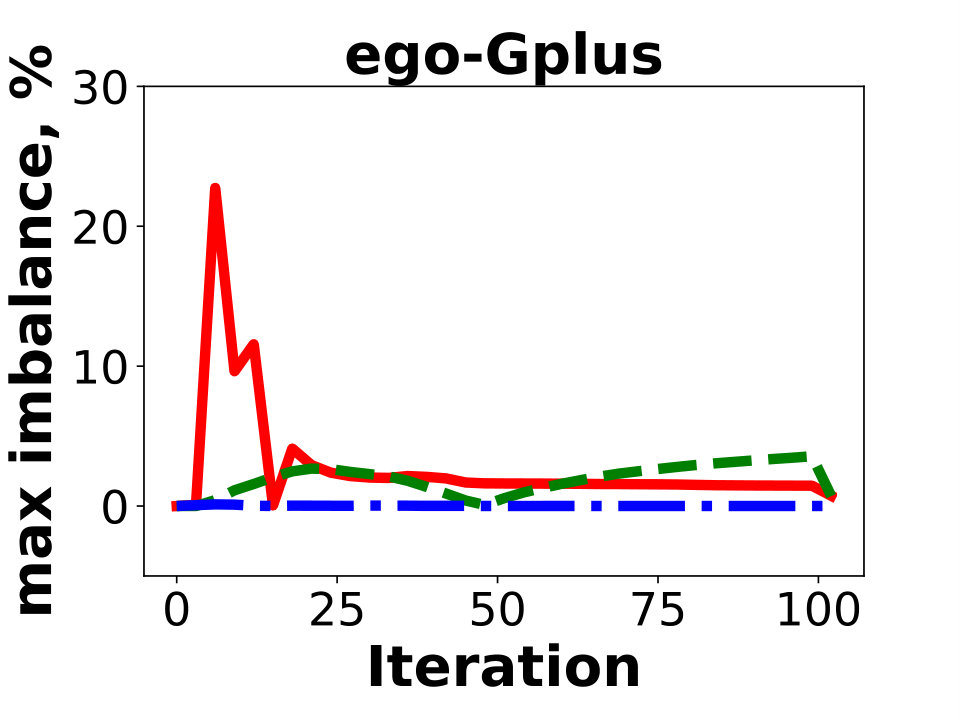 Figure 4
 Figure 5
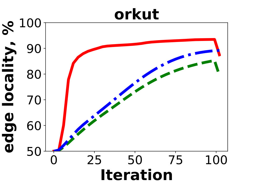 Figure 6
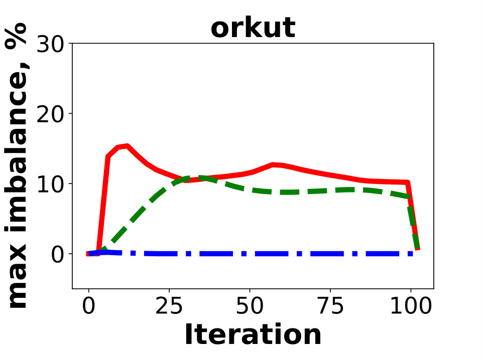 Figure 7
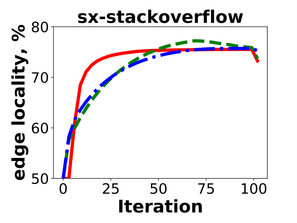 Figure 8
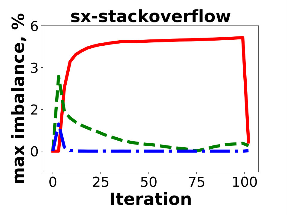 Figure 9
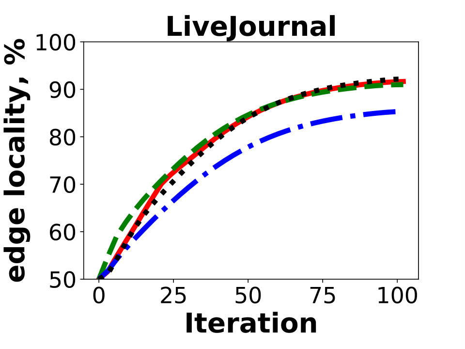 Figure 10
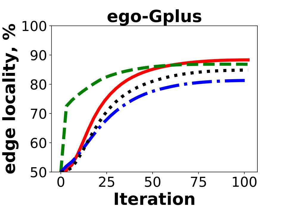 Figure 11
 Figure 12
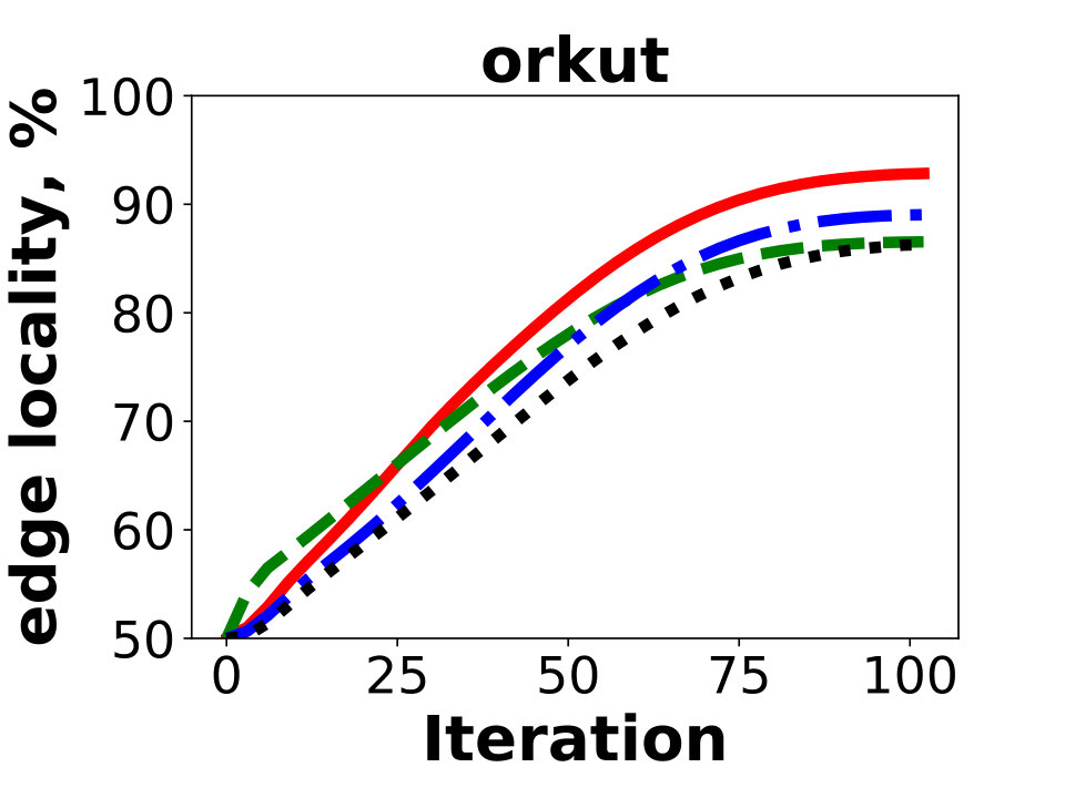 Figure 13
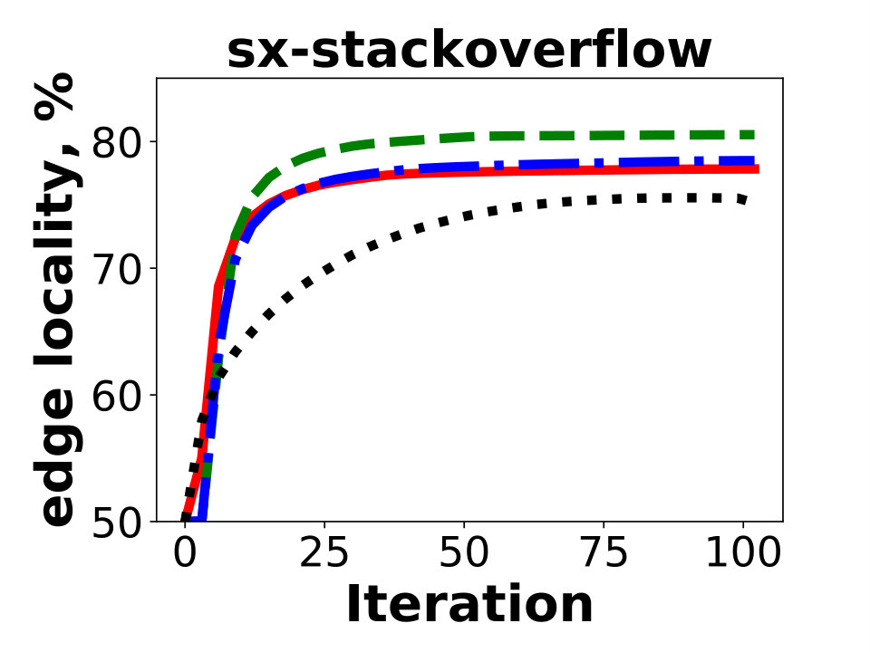 Figure 14
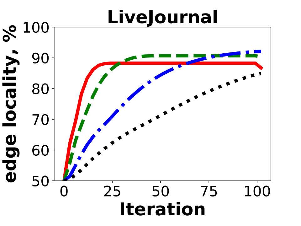 Figure 15
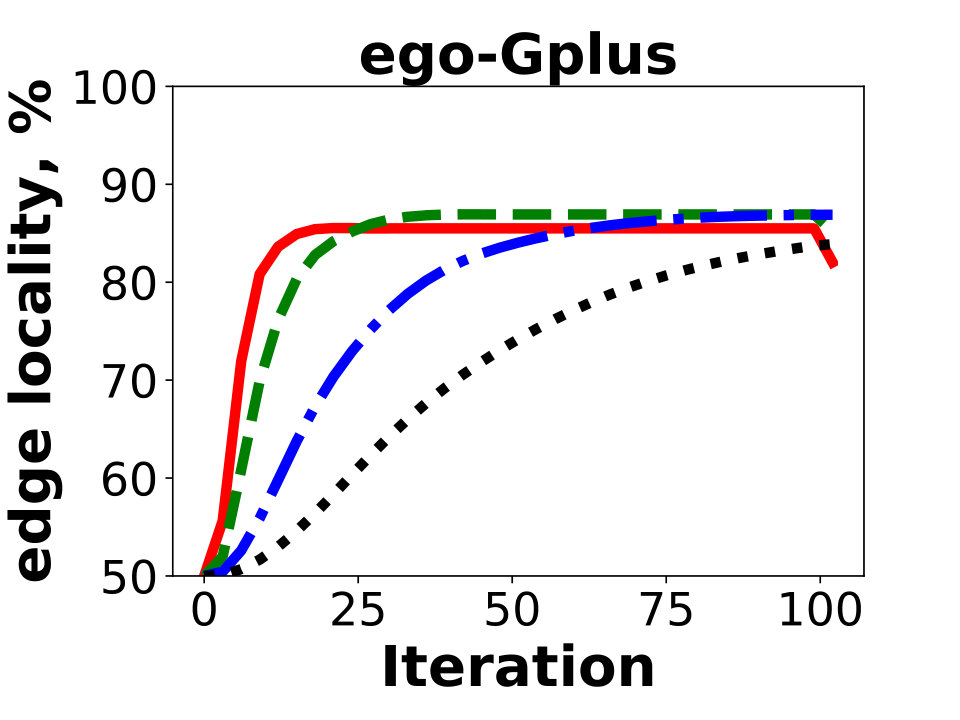 Figure 16
 Figure 17
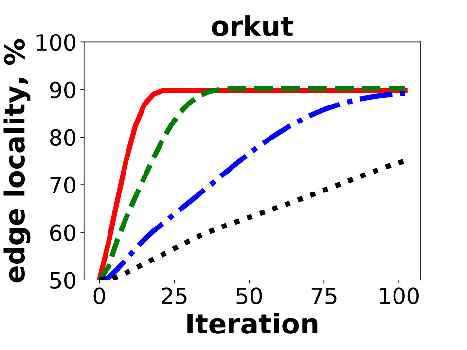 Figure 18
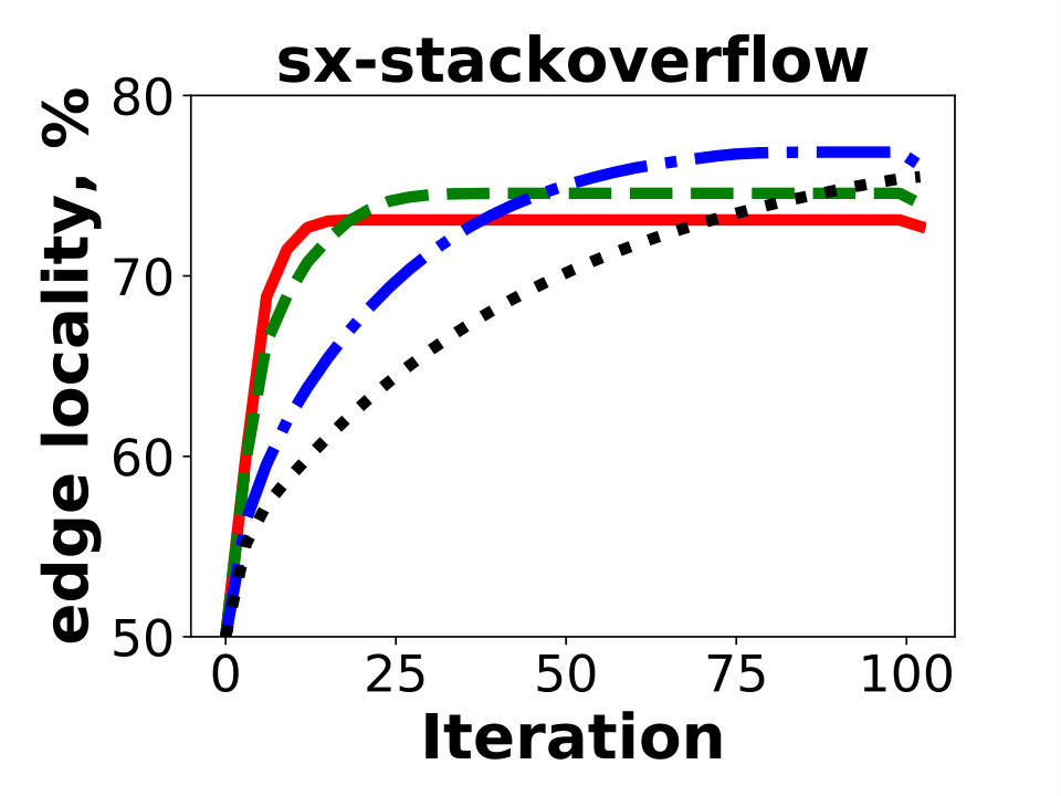 Figure 19
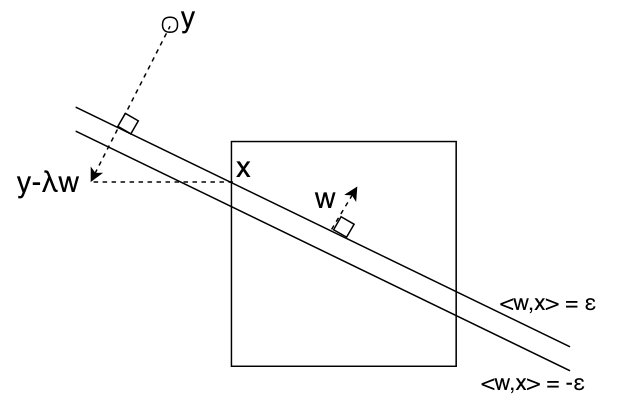 Figure 20
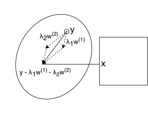 Figure 21
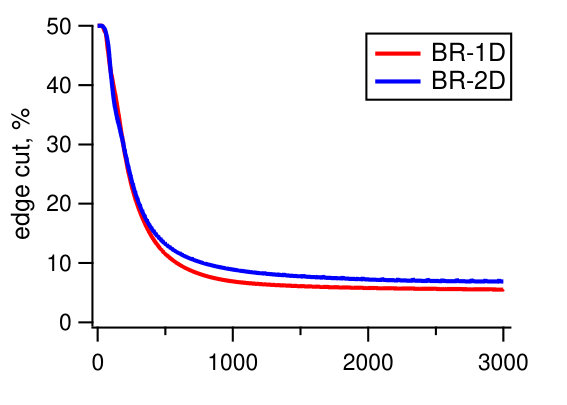 Figure 22
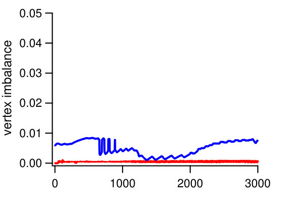 Figure 23
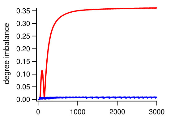 Figure 24
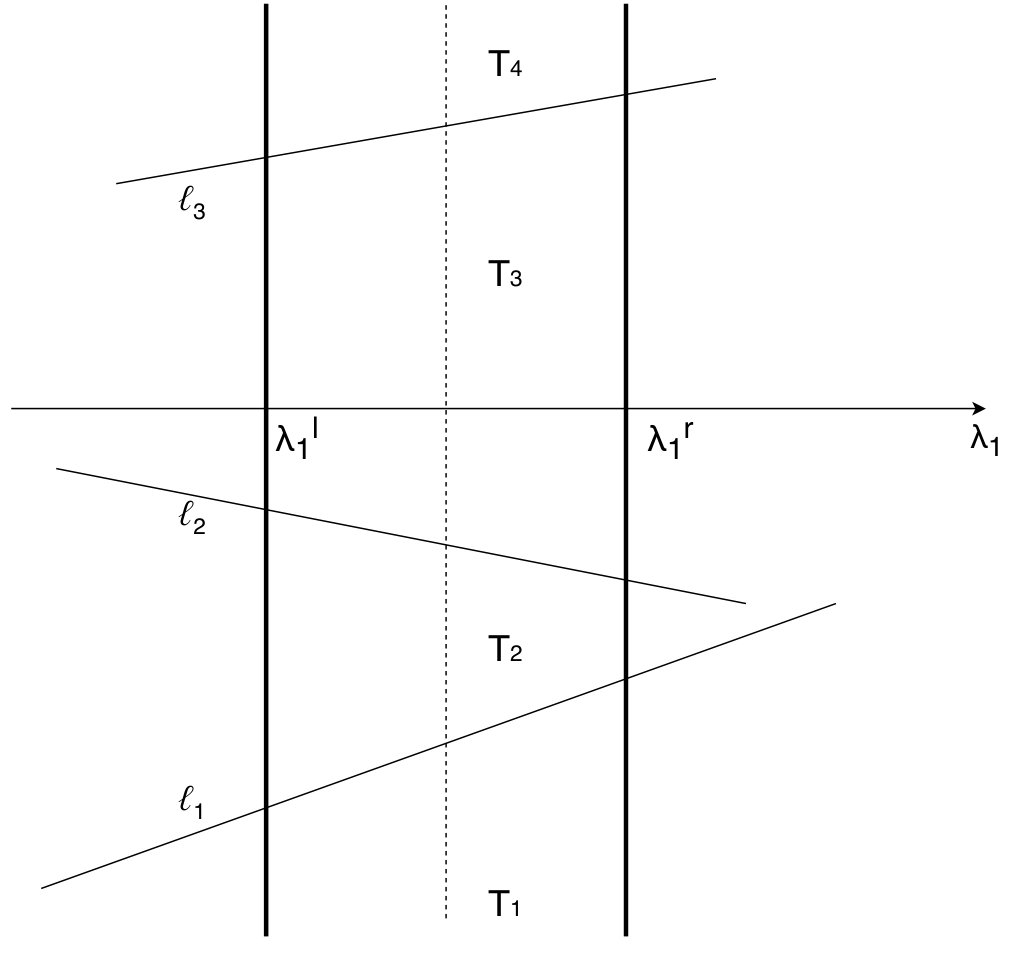 Figure 25
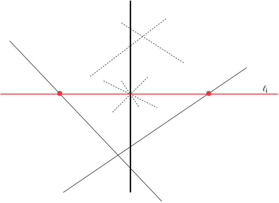 Figure 26
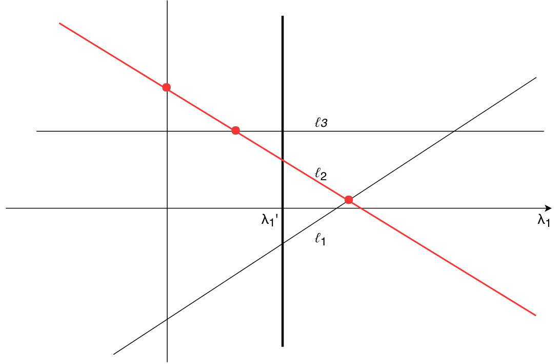 Figure 27
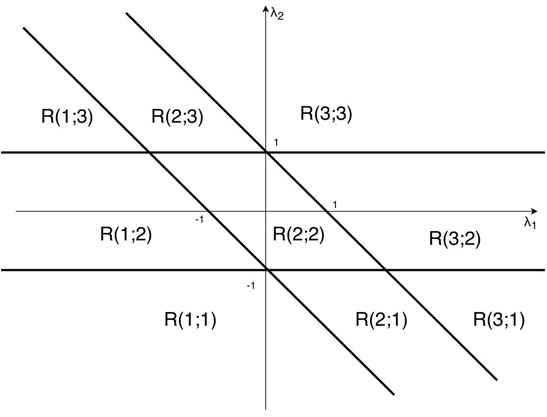 Figure 28
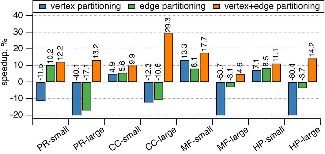 Figure 29
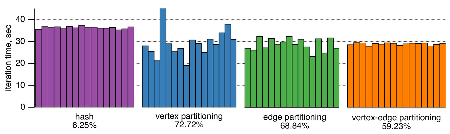 Figure 30
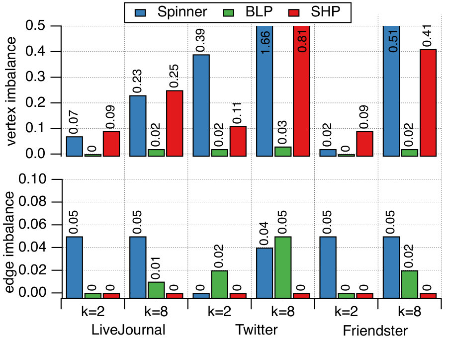 Figure 31
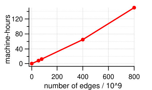 Figure 32
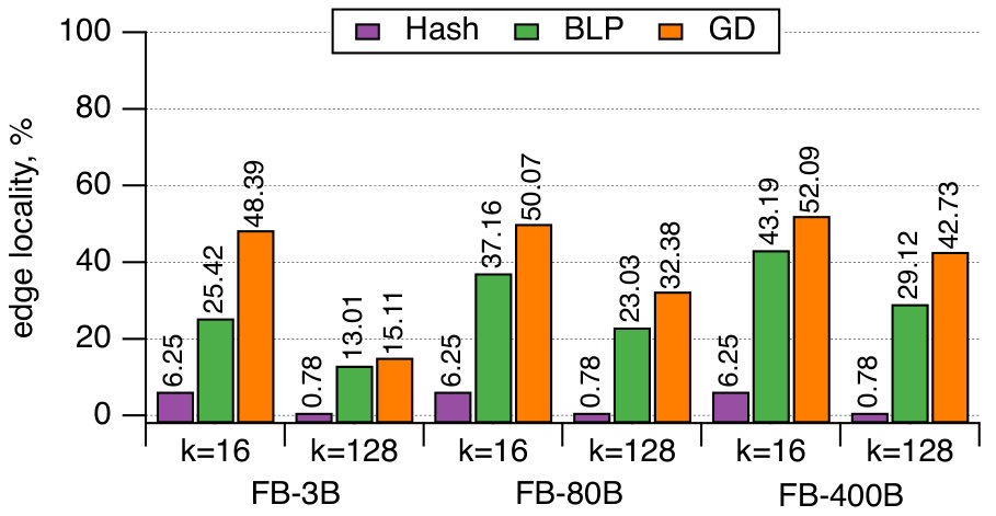 Figure 33
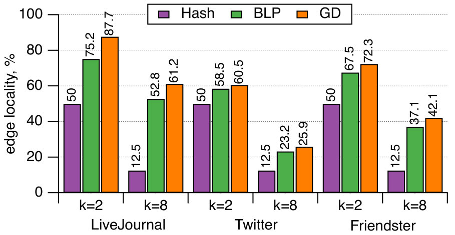 Figure 34
| Output | Time required | ||
| Alternating | any | Until convergence | |
| Dykstra’s | any | projection | Until convergence |
| Exact (ours) | projection |
| Partitioning | Runtime, sec | Communication, GB | ||||
| mean | max | stdev | mean | max | stdev | |
| Hash | ||||||
| vertex | ||||||
| edge | ||||||
| vertex-edge | ||||||
| LiveJournal | orkut | sx-stackoverflow | |||||
| GD | METIS | GD | METIS | GD | METIS | ||
| : balance on vertices and degrees | Locality, | ||||||
| imbalance, | |||||||
| Memory, MB | |||||||
| Time, s | |||||||
| : balance on vertices, degrees and sum of neighbor degrees | Locality, | ||||||
| imbalance, | |||||||
| Memory, MB | |||||||
| Time, s | |||||||
| : balance on vertices, degrees, sum of neighbor degrees and pagerank | Locality | ||||||
| imbalance, | |||||||
| Memory, MB | |||||||
| Time, s | |||||||
Peer Reviews
No public reviews on file for this paper yet. If you reviewed it on a platform where reviews are public (OpenReview, ICLR, NeurIPS, ICML), you can paste yours below so the community can read it here.
Videos
No videos yet. Explain this paper in a talk, walkthrough, or lecture? Add one.
\usetkzobj
all
Multi-Dimensional Balanced Graph Partitioning via Projected Gradient Descent
Dmitrii Avdiukhin
Sergey Pupyrev
Grigory Yaroslavtsev
Indiana University
Bloomington, IN
Menlo Park, CA
Indiana University
Bloomington, IN
Abstract
Motivated by performance optimization of large-scale graph processing systems that distribute the graph across multiple machines, we consider the balanced graph partitioning problem. Compared to most of the previous work, we study the multi-dimensional variant when balance according to multiple weight functions is required. As we demonstrate by experimental evaluation, such multi-dimensional balance is essential for achieving performance improvements for typical distributed graph processing workloads.
We propose a new scalable technique for the multi-dimensional balanced graph partitioning problem. The method is based on applying randomized projected gradient descent to a non-convex continuous relaxation of the objective. We show how to implement the new algorithm efficiently in both theory and practice utilizing various approaches for the projection step. Experiments with large-scale graphs with up to 800B edges indicate that our algorithm has superior performance compared with the state-of-the-art approaches.
1 Introduction
Distributed graph processing systems have been widely adopted in recent years to enable analysis and knowledge extraction from large-scale graphs. Systems such as Giraph [6], GraphX [19], GraphLab [30], and PowerGraph [18] allow users to use a vertex-centric model for applications which can be executed on a cluster of worker nodes. In this setting, each worker node operates on a subset of the input graph and communicates with other workers by sending messages. The process of splitting the input graph into these subsets, also known as graph partitioning, is essential for optimizing performance of such systems [18, 43, 20, 3].
Created partitions have a significant impact on the communication between different workers and the resource usage of individual workers. In order to maximize the processing speed, the partitions should largely be independent to minimize communication. At the same time, computation executed on each partition should take approximately the same amount of processing time, as the overall performance depends on the slowest worker. These constraints give rise to the Balanced Graph Partitioning problem whose goal is to divide the vertices of a graph into a given number of (approximately) equal size components while minimizing the resulting edge cut. Balanced Graph Partitioning is a classic and thoroughly studied problem from both theoretical and practical points of view [9, 12]. In the context of distributed graph processing, the problem is typically studied in two variants.
In the vertex partitioning model, each worker machine is assigned an equal number of vertices with the goal of minimizing the number of cross-machine edges. Since messages are usually sent between adjacent vertices, storing tightly connected subgraphs on the same worker can reduce communication and hence running times of jobs. It has however been observed that this strategy does not lead to equally loaded partitions for real-world graphs with power law degree distribution [18]. Graph partitioning algorithms tend to colocate high-degree vertices and corresponding partitions take much longer to process, resulting in longer execution time overall.
The edge partitioning model has been suggested to alleviate the above imbalance problem [18, 29]. In this model the goal is to partition the graph so that the number of edges in every component is the same, while the number of incident edges across different components is minimized. Good partitions according to this model typically result in better balance across workers and reduced computation time in comparison to the trivial hash-based assignment of vertices to worker machines. However, edge-based graph partitioning can still result in performance regressions [3, 40].
To analyze the source of regressions, we performed a simple experiment of running a Page Rank algorithm implemented on top of Giraph utilizing various graph partitioning methods. Figure 1 illustrates the histograms of running times for individual workers processing a graph with vertices and edges. As discussed above, partitions according to the vertex partitioning model suffer from unequal distribution of edges across workers. A single overloaded partition can contain x more edges than an average one, which results in x longer execution time. We also observe a high correlation () between the number of edges assigned to a partition and the corresponding processing time in this experiment. Partitioning according to the edge partitioning model yields a x running time improvement over the baseline, though there is still a noticeable imbalance between the fastest and the slowest worker machines. This can be explained by uneven distribution of vertices among workers. Machines with more vertices have higher operational overhead such as serialization of sent messages whose number is proportional to the number of vertices on a worker. Here we observe an x imbalance in the number of vertices and a moderate correlation () between the running time and the vertex count on the workers.
In order to mitigate the issues described above we introduce a new strategy, vertex-edge partitioning, which is designed to balance the number of vertices and edges across workers simultaneously. As shown in Figure 1, this is done at a cost of a lower edge locality (percentage of edges with both endpoints on the same machine), and thus, higher communication volume. The resulting assignment results in a x speedup over the hash-based model. Motivated by the above experiment and a number of earlier studies [43, 20, 3, 40], we formalize a new model for graph partitioning which is suitable for real-world distributed graph processing systems.
We now formally describe the model in the most general setting which allows one to require balance according to different unrelated weight functions. Let be a graph with vertex weight functions , each assigning a positive weight to every vertex in the graph. Let be the sum of weights of all vertices in the graph according to the -th weight function. Given an integer and a parameter , the goal is to find a partition of the vertex set into sets such that for each weight function and each part of the partition the sum of weights in is approximately the same and close to the average, i.e. . We call such partitions -balanced. Finally, among all such -balanced partitions the goal is to find one that maximizes the number of edges whose both endpoints are contained within some part of the partition and hence minimizes the size of the cut. This problem is referred to as Multi-Dimensional Balanced Graph Partitioning (MDBGP).
The simplest example of MDBGP is the classic balanced graph partitioning problem which is equivalent ot the vertex partitioning strategy described above and can be expressed using a single weight function . Since this requires that we maximize edge locality while ensuring that . Using two weight functions and corresponds to requiring balance on the number of vertices and edges in the parts of the partition and hence corresponds to the vertex-edge partitioning approach described above. Indeed, and hence in addition to balance on the number of vertices this requires that . However, the model is not restricted to vertex- and edge-balance (as in the aforementioned vertex-edge partitioning) but can take arbitrary user-specified weights. In particular, when partitioning the vertices of the graph between the workers for load balancing, various weights modeling expected vertex activity can be used (historical data on individual vertex load, proxy values for the load such as PageRank, etc).
While a large body of work exists offering practical solutions for the one-dimensional version of the problem [23, 13, 42, 41, 7, 14, 33, 22, 12], as well as on theoretical foundations of graph partitioning [26, 4, 32], literature on principled and scalable approaches for the multi-dimensional case is quite sparse [24, 37, 36, 35]. In particular, if the weight functions are unrelated to each other, one can easily construct examples when no feasible solution exists that satisfies all balance constraints even for two weight functions. However, it is empirically observed that instances coming from applications often allow balanced solutions for several weight functions of interest simultaneously. For classical local search based algorithms such as [25] handling of multiple unrelated weight functions is challenging since imposing one balance constraint might violate another and hence finding a good local move becomes computationally hard. We overcome this difficulty by using a continuous relaxation of the problem, which allows more flexibility for achieving balance in the search space. In order to obtain an integral solution, in the end we apply randomized rounding which preserves balance with high probability.
1.1 Our Contributions
We present a scalable algorithmic framework for the problem of balanced partitioning of large graphs according to multiple user-specified weight functions while maximizing the number of edges inside the resulting components. Our framework consists of applying the projected gradient descent on a standard relaxation with a suitably chosen projection method. The relaxation is to maximize a non-convex quadratic function for , where is the adjacency matrix, subject to a constraint for a certain convex body defined by the weight functions. Section 2 provides the exact description of the relaxation. Note that the gradient descent step only uses a matrix-vector multiplication since , and thus, the algorithm allows a straightforward distributed implementation.
While applying projected gradient descent to solve non-convex optimization problems subject to convex constraints is a well-studied approach in non-linear optimization (Section 2.3, [8]) and machine learning (Section 6.6, [21]), one has to overcome two technical challenges to make it applicable to the multi-dimensional graph partitioning problem: 1) projection step is computationally expensive, 2) existence of points with small gradient (saddle points) slows down convergence.
We show how to address the first challenge by designing efficient projection step algorithms tailored to the standard relaxation of MDBGP. While convergence to the projection point can be achieved using various alternating projections methods [15], for we give one-shot exact solutions with almost linear running time.
Theorem 1.1
Running time of the projected gradient descent step is for and scales as when distributed between machines.
In order to address the second challenge, we use small perturbations to get out of saddle points, where the perturbation vectors are sampled from a scaled -dimensional Gaussian distribution. We refer to the resulting algorithm as GD, see Algorithm 1. Convergence analysis of GD remains an open problem. While noisy gradient descent is known to have fast convergence to a local optimum for non-convex optimization subject to equality constraints, if inequality constraints are allowed convergence analysis is unknown [16].
Our experimental results show that GD scales to graphs with up to several billions of vertices and up to edges. We conducted an experimental evaluation of various graph partitioning strategies for optimizing several real-world Giraph workloads. The results demonstrate that multi-dimensional balancing is a suitable objective for achieving performance improvements, providing speedups in the order of over the state-of-the-art one-dimensional partitioning strategies. Compared to existing scalable graph partitioners, such as Social Hash Partitioner [22], Spinner [33], and Balanced Label Propagation [42, 34], the algorithm is conceptually simple and obtains close-to-perfect balanced partitions across multiple dimensions.
1.2 Previous Work
While one-dimensional balanced graph partitioning has been studied extensively and a number of tools exist [23, 13, 42, 41, 7, 14, 33, 22] (see also surveys by Bichot and Siarry [9] and by Buluç et al. [12]), to the best of our knowledge none of the practical algorithms for this problem have been previously based on running gradient descent on a continuous relaxation. Existing approaches are inherently discrete and are based on combinations of various discrete algorithms: greedy heuristics (METIS [23], Fennel [41]), branch-and-bound [13], label propagation and local search (balanced label propagation [42], Social Hash Partitioner [22], Spinner [33]), as well as hybrid approaches (linear embedding method combined with various optimizations [7]). Due to the combinatorial nature of these algorithms, their generalizations to the multi-dimensional case appear to be non-straightforward without substantial losses in performance, while our continuous relaxation handles multiple balance constraints uniformly. Compared to the one-dimensional version, existing literature on the multi-dimensional version is rather sparse [24, 37, 36, 35] and the main publicly available tool for the problem is currently METIS [24, 37].
Vast literature exists on optimization of non-convex functions and the interest in this topic lately has been particularly high. However, in the constrained case when the optimization has to be performed over a convex body, fairly little is known; see classic optimization literature [8, 44, 11]. Recent results on the non-convex optimization problem subject to convex constraints and its special cases include [16, 39, 5, 17, 21]. Closest to our work in terms of techniques is [27] who use projected gradient method to solve convex programs involving the max-norm and show how to solve large semidefinite programming relaxations of Max-Cut. Their results are quite different from ours as we consider a balanced version of graph partitioning and expect our algorithms to be scalable; the largest instances handled by [27] have and . Since we require that our algorithms scale to graphs with billions of edges, using existing general purpose software for constrained quadratic programming is also infeasible.
2 Projected Gradient Descent
For an integer we use notation to denote the set . The weighted -dimensional balanced graph partitioning problem is defined by a collection of weight functions , where . For a set we use notation .
Definition 2.1** (MDBGP)**
Given a graph , an integer and a parameter , the Multi-Dimensional -Balanced Graph -Partitioning problem is to find a partition of the vertex set into sets such that for each , it holds that for all . Among all such partitions the goal is to find one that maximizes the number of edges whose both endpoints are contained within some part of the partition.
In this paper we focus on the -partitioning problem; for the general variant of -partitioning, we apply the algorithm recursively. For MDBGP is equivalent to the following integer quadratic program:
Maximize:
Subject to:
The interpretation of variables is that if then and if then . The objective is then the same as in MDBGP and counts the number of edges whose both endpoints are contained in some part of the partition. Indeed, an edge makes a contribution of to the objective when (and hence ) and [math], otherwise (since ). The constraints are equivalent to . Adding or subtracting to both sides and dividing by we have as required in MDBGP.
After dropping the additive term the objective can be expressed as and has gradient and Hessian . Finally, we use a continuous relaxation of the above problem where we replace the integrality constraints with for all . A solution to this continuous relaxation can be converted into an integral solution using randomized rounding. Using independent random variables for each vertex such that and the expected value of the objective on the rounded solution is the same as on the initial fractional solution while all balance constraints are still approximately preserved with high probability by concentration bounds.
2.1 Overview
We propose the following algorithm for the multi-dimensional balanced graph partitioning problem based on the continuous relaxation described above. The algorithm is referred to as Gradient Descent (GD), see Algorithm 1. It computes a sequence of vectors , where for all and . Here is initialized with zero vector, and is computed by applying projected gradient descent iteration to . Each iteration consists of three steps.
Step 1: Adding noise. We add Gaussian noise to obtaining a noisy vector . The noise is drawn from the -dimensional Gaussian distribution with zero mean and variance in each coordinate. The addition of noise to allows to escape from saddle points, e.g. .
Step 2: Gradient descent. We obtain from the noisy vector via a gradient descent step with step size . Note that the gradient at is given as hence this step can be expressed as .
Step 3: Projection. The resulting vector is then projected on the feasible space , where:
[TABLE]
that is, satisfies that and corresponds to the constraints imposed by the balance of weights according to the -th weight function.
The final solution is obtained by rounding last : each vertex is assigned to part with probability . Note that this ensures that the expected number of edges whose endpoints belong to the same part after this rounding is given as .
The algorithm uses parameters , and , where is the iteration index. Here controls the magnitude of noise, is the step size, and is the number of iterations. We discuss the selection of parameters in the experimental Section 4.
2.2 Projection
In the projection step of GD (Line 1) we need to find , where . Denoting as we formulate this step as an optimization problem:
Minimize:
Subject to:
The optimum solution to the optimization problem has to satisfy KKT conditions:
Stationarity:
Complementary slackness 1:
Complementary slackness 2:
Here are the dual variables and is the -th standard unit vector. It is a standard fact (see [11], Chapter 5.5.3) that for convex optimization subject to linear constraints Stationarity, Complementary slackness and Primal/Dual feasibility are necessary and sufficient conditions for the optimum solution. Thus we just focus on satisfying these conditions below.
Let . Then by Stationarity for each we have . Consider the following three cases:
Case 1. . If then by Stationarity which violates primal feasibility conditions. Therefore and by Complementary slackness 1. Among the two roots and the second root can be ruled out and hence . Indeed, if then by Stationarity which contradicts and .
Case 2. . This case is symmetric to the previous one and thus in this case.
Case 3. . First we show that . Indeed, assume that . Then by Complementary slackness 1. Both cases lead to contradiction:
. By Stationarity which contradicts with and . 2. 2.
. Similarly to the above by Stationarity we have which is a contradiction with and .
Therefore in this case we have and hence by Stationarity .
Let and assume that these values are known to the algorithm. For we use notation for the truncated linear function. Using the analysis above the projection step is simply . It remains to show how to find .
Note that from Complementary slackness 2 it follows that either or since both of these values being positive leads to a contradiction. This leads to three cases: 1) , 2) and 3) which correspond to the three possibilities for . For each of the dimensions we can try all three choices. For a fixed guess of the signs let , and . Assuming a correct guess of for each of the dimensions the optimization problem above reduces to the following:
Proposition 2.1
For the correct guess of for all it suffices to find the optimum of the above optimization problem without the constraints for . This optimum is unique.
The proof is given Appendix B. Using Proposition 2.1 and trying all guesses for we can reduce the projection step to instances of the following optimization problem:
Minimize:
Subject to:
which can be done by finding numbers for and for and setting . The choice of ’s has to satisfy the constraints for all and for all . In the analysis below we assume that corresponds to the “effective dimension” of the problem.
2.3 Exact Projection Algorithms
Projection for
As a warm up, we first show how to perform exact projection for in time, proving Theorem 1.1 for . This can be further improved to using a more careful approach [31]. However, to the best of our knowledge, no fast algorithm is known for which is the main focus of our work. Dropping the second index to simplify presentation (that is, ) and using the fact that we have:
[TABLE]
We introduce notation where each is the following piecewise linear function:
[TABLE]
Thus and the problem reduces to finding such that where the sign depends on whether our dimension is in or . Since for all each is monotone in and so the function is a monotone piecewise linear function. The value of can be found in iterations of binary search where each iteration requires time to evaluate the sum. This gives the overall running time of . See Figure 2 for an illustration.
Projection for
For we need to find such that for , where is defined below.
[TABLE]
where . The projection process is shown in Figure 3. In Appendix A.2, we prove Theorem 1.1 for showing that nested binary search can be used to solve this problem in time.
3 Implementation
3.1 Projection algorithms
We considered the following three methods for the projection step (Algorithm 1, Line 1). Their theoretical properties are summarized in Table 1.
- •
Alternating projections: A standard approach for projection on the intersection of convex sets is the alternating projections method (see [10]). It is easy to implement projections on and separately. Since both are convex bodies by alternating projections on each of them one can guarantee convergence to a point in the intersection, but there is no guarantee that this point will be the actual projection. In practice, we are able to achieve slightly better balance by modifying this approach slightly and projecting on instead of . This still ensures that we get a point in the intersection in the end.
- •
Dykstra’s projection: [1] We also considered Dykstra’s projection algorithm [15]. This is a modification of the alternating projections method which is guaranteed to converge to the projection.
- •
Exact projection for : This is the algorithm presented in Section 2.2. In our experiments Dykstra’s algorithm and exact projection give similar results, since they find approximately the same projection point.
In Section 4.3 we study how quality of partitions produced by GD depends on choice of one of the projection methods above. Since the exact projection algorithm is computationally the most expensive, in our experiments we mostly use the alternating projections method. Moreover, since in practice each iteration of alternating projection is computationally expensive, in the intermediate iterations we project on each plane and the cube only once, while in the last iterations we run the alternating projections method until convergence. We refer to this choice as “one-shot” alternating projection below.
3.2 Adaptive Step Size
Recall that Algorithm 1 has the following parameters: Gaussian noise variances for each step and step size parameters . Due to the spectral properties of the adjacency matrix in our experiments the algorithm doesn’t encounter any saddle points other than the initial point . Therefore it suffices to add Gaussian noise only at first iteration (that is, for ).
The simplest choice of the step size parameters is constant, but it gives suboptimal results in our experiments. Carefully chosen step size parameters for different iterations not only gives better performance but can also be used to ensure that convergence can be reached in a fixed number of steps. In section 4.3 we discuss how to choose the step size to achieve good performance on a wide range of graphs.
The choice of step size parameters is complicated by the projection step. The change in the objective function and the progress towards an integral solution can both be related to the progress in Euclidean distance between the iterations. While consistent progress in Euclidean distance can be ensured by multiplying the gradient by an appropriate amount after the projection the actual progress can be much smaller.
Another important implementation detail is our handling of vertices which are close to integral. When the number of such vertices becomes large the progress of the algorithm can slow down. This is due to the fact that while the gradient vector is still large all of its large components correspond to already integral vertices and point to the outside of the feasible region. These large components can then dominate in the computation of the projection step which leads to slow convergence. In order to avoid this issue we “fix” such vertices so that they become integral and no longer participate in the gradient update and the projection step. As we show in Section 4.3 this results in noticeable improvements in the quality of the resulting partitions.
3.3 Partitioning Into k Buckets
For partitioning into more than two buckets two main approaches are typically considered. We use the second approach due to its higher efficiency.
Problem relaxation for buckets: For each vertex and bucket we can introduce a variable corresponding to whether belongs to bucket and then adjust the relaxation accordingly. Our algorithm GD can then be modified to handle such relaxation. The main drawback of this approach is that it requires communication per iteration, which makes it infeasible for partitioning large graphs into many buckets.
Recursive partitioning: The graph is partitioned recursively times into two parts. While there are cases when recursive partitioning can result in a suboptimal partition regardless of the underlying algorithm, this approach requires memory, operations per iteration and runs of GD, which makes it applicable to very large graphs. For simplicity we only show results for being powers of two but the algorithm can be modified to handle any by changing the coefficients in the balance constraints.
4 Experiments
We design our experiments to understand how well the new partitioning algorithm, GD, behaves on real-world datasets and how it affects the performance of distributed graph processing. As pointed out in Section 1, we are not aware of an alternative scalable approach for solving the multi-dimensional balanced partitioning. However, some of the existing techniques for one-dimensional partitioning can be adapted for the multi-dimensional case. Next we discuss several such techniques, which are evaluated together with the newly proposed algorithm.
Hash is the simplest partitioning strategy that assigns vertices to worker machines by hashing the vertex identifiers. Hashing is stateless, extremely fast in practice, and requires no preprocessing of the graph, which made it the default strategy in Giraph. The main disadvantage is that the majority of sent messages are non-local and may results in significant communication.
Spinner is a graph partitioning algorithm that can be applied to process large-scale graphs in a distributed environment [33]. The algorithm is based on the label propagation technique in which vertices exchange their labels trying to pick the most frequent label among its neighbors. This process guarantees a high number of adjacent vertices having the same label, which are then assigned to the same worker. Spinner does not enforce a strict balance across partitions but integrates score functions that penalize imbalanced solutions.
BLP is another approach based on the balanced label propagation based on combining the ideas of Ugander and Backstrom [42] and Meyerhenke et al. [34]. On the first step, the method creates a size-constrained clustering of the input graph using significantly more clusters than the number of available machines, . In our implementation, we construct clusters for and forbid a cluster to contain more than vertices and edges. On the second step, we randomly merge the clusters into partitions, which results in the multi-dimensional balance even if the original clusters have different sizes.
SHP is a distributed graph partitioner [38, 22] that is based on a classical local search heuristic [25]. Although SHP does not provide balancing on multiple dimensions, it supports a mode with several dimensions whose final balance is not guaranteed. The algorithm works by balancing on a new dimension, which is a combination of the specified dimensions. We configure SHP to find solutions having the same number of edges (with a higher coefficient in the combination) and the same number of vertices (with a lower coefficient) in every partition.
We implemented the algorithms and extensively experimented with the Giraph framework, which is used as the primary tool for large-scale graph analytics at Facebook [6, 2]. Although the evaluation is performed with the single distributed graph processing system, we believe that our main conclusions are valid for other frameworks relying on the vertex-centric programming model. For our experiments, we use four large social networks that are publicly available [28]. LiveJournal, Orkut, Twitter, and Friendster are undirected graphs containing , , , and million of vertices and , , , and billion of edges, respectively. In addition, we experiment with several large subgraphs of the Facebook friendship graph that serve to demonstrate scalability of our approach and its performance on real-world data. We denote the graphs by FB-X, where X indicates the (approximate) number of billions of edges; this data is anonymized before processing.
Next we analyze the quality of the solutions produced by the algorithms on our dataset (Section 4.1) and evaluate various graph partitioning strategies for speeding up distributed graph processing for real-world workloads (Section 4.2). Section 4.3 investigates various parameters of GD.
4.1 Multi-Dimensional Partitioning
Our initial experiments (see Figure 1) and earlier works [18, 29, 33] indicate that two important dimensions for the performance of Giraph jobs are the number of vertices and the number of edges. For this reason, we specify two weights for the vertices, and for all . Recall that our primary goal is to guarantee almost perfect balance for the two dimensions, as even a single overloaded partition affects the job performance. Figure 4 illustrates the resulting vertex and edge imbalance of the solutions on the public networks for three algorithms, Spinner, BLP, and SHP, using and partitions. The imbalance is defined as , where the maximum and the average are taken over the total weight of all constructed partitions. We do not include the results for Hash and GD, as the corresponding values are below for the instances.
We observe that two algorithms, Spinner and SHP, are not suitable for the multi-dimensional variant of the problem. For dense graphs with a highly skewed degree distribution (as in Twitter), the algorithms cannot simultaneously provide balance on the two dimensions. With the default setting, these two algorithms generate solutions in which some of the partitions contain x more vertices than the average one. We tried to modify the techniques by adjusting relative weights of their penalty functions for vertex and degree counts in resulting partitions. However, we were not able to design universal penalty weights that work for all instances. A similar behavior regarding the resulting balance is observed for our internal graphs, FB-3B, FB-80B, and FB-400B. In contrast, Hash, GD, and BLP produced nearly-balanced (that is, having both for vertex and edge counts) solutions for all the instances. With this in mind, we exclude Spinner and SHP from further experiments.
Next we compare the quality of our algorithm as measured by the resulting edge locality, that is, the percentage of uncut edges with both endpoints in the same partition. The metric represents the fraction of local messages in Giraph jobs and corresponds to a possible reduction in communication between the worker machines. Figure 5 reports the results of Hash, GD, and BLP on the public dataset. Unsurprisingly, GD and BLP outperform the Hash algorithm in the experiment, as the latter keeps only of all the edges in the same partition. The resulting edge locality of GD and BLP are close for the three graphs, though GD typically achieves a higher locality by .
Figure 6 shows the experiments on the Facebook friendship graphs. Here we use a larger number of partitions, , which more accurately represent the real-world Giraph use case. Again, Hash produces solutions having the lowest edge localities. In fact, over of the edges are cut using the partitioning strategy for an instance with a hundred partitions. This is in agreement with our measurements of the typical percentage of cross-worker Giraph messages in the production environment.
On the other hand, we observe a bigger advantage of GD over BLP; the locality difference is around for and for . The balanced label propagation algorithm, BLP, could be configured to produce better results by decreasing its cluster size threshold, . However, this results in an imbalanced solution with for the largest instance with . Hence, we keep the value of for all the experiments.
The main difference between FB graphs and publicly available graphs is the number of edges. The main reason why on FB graphs GD performs better compared to other algorithms is poor performance of existing local-search based methods on large graphs in the multi-dimensional case. This is most obvious in Figure 6 for as one can see that GD is gaining a larger advantage over BLP as the size of the graph grows (3B 80B 400B).
Overall we conclude that GD generates solutions of higher quality than BLP and Hash on all examined instances. Therefore, we utilize the algorithm to experiment with distributed graph processing in the next section. We present results for - and -dimensional experiments in Appendix C.
4.2 Distributed Graph Processing
In this section we conduct an experimental evaluation of various graph partitioning strategies for speeding up distributed graph processing. Here we argue and experimentally demonstrate that multi-dimensional balancing is a suitable objective for the application. We experiment with four graph algorithms implemented in Giraph. Page Rank and Connected Components, are popular benchmarks for verifying the performance of distributed systems. Page Rank iteratively propagates vertex ranks through adjacent edges; our implementation performs iterations for the algorithm. For the Connected Components algorithm, we use a simple label propagation technique in which vertices iteratively update their labels based on the minimum label of their neighbors; for our graphs, the process converges after at most rounds. The other two algorithms, Hypergraph Clustering and Mutual Friends, are production applications for large-scale graph analytics at Facebook. The former is used to find a certain clustering of the input graph by converting it to a hypergraph. The latter builds a set of features for friend recommendation on Facebook. Both applications extensively exchange messages between adjacent vertices, which adds a significant communication overhead.
Figure 7 depicts the results of our experiment. Since we are interested in the impact of various partitioning policies on the performance of Giraph, we report the relative differences to the baseline policy, Hash. Here we measure the total runtime of an application using GD as the partitioning strategy in three modes, vertex partitioning (one-dimensional balance on vertex count), edge partitioning (balance on edge count), and vertex-edge partitioning (two-dimensional balance both on vertex and edge counts). Every algorithm is applied in two configurations, small and large. The first one uses the FB-80B graph and a cluster with worker machines, while the second one process FB-400B using workers.
The key finding is that one-dimensional partitioning cannot provide consistent benefits across all the Giraph applications. In fact, we observe performance regression for some instances, in particular, when the number of utilized worker machines is large, that is, . In this scenario, we notice a few workers whose running time is significantly larger than the average; see Figure 1. Since in Giraph (and other vertex-centric systems) the computation is split into a number of supersteps that end with a global synchronization barrier, the performance is determined by the slowest worker. Notice that a similar phenomena regarding the vertex partitioning has been observed in earlier works [18, 3, 40, 20]. In contrast, the two-dimensional partitioning always results in a speedup over the default Hash strategy. The improvement is in the order of for the examined applications.
To get a deeper understanding of the source of performance differences, we analyze the detailed logs for the Page Rank application using a cluster with worker machines. Table 2 shows the measurements of the mean, maximum, and standard deviation of the time to compute a superstep by all the workers. The results indicate that the with hash partitioning the workers are idling on average for seconds per superstep waiting for the slowest one to complete the work. With one-dimensional partitioning the idling time is much longer, seconds for vertex-based partitioning and seconds for edge-based one, which is the primary reason for the performance regression. The two-dimensional partitioning results in a more even load across the workers delivering a speedup. Table 2 also indicates a significant communication reduction over the baseline partitioning, as measured by the total size of messages sent between the workers via network. For the Page Rank application, the average reduction is correlated with the edge locality of the corresponding partitioning. However, an unbalanced partitioning causes some workers to use more memory resources and become a bottleneck for graph processing.
Finally, we emphasize that the timings analyzed in the section exclude the running times of the partitioner itself. This is realistic for our use case in which the same friendship graph is expected to be processed multiple times for various analytics tasks. Thus, the extra overhead incurred by a partitioning strategy is amortized among several runs.
4.3 Parameters of GD
In this section we perform an experimental comparison of various choices of the projection step algorithm in GD and study its convergence properties. Unless specified otherwise, we use two-dimensional GD in the following setting:
- balance is required with respect to the number of vertices and their degrees,
- in the projection step we use “one-shot” alternating projection (see Section 3.1),
- we use adaptive step size and vertex fixing as described in Section 3.2.
Since behavior of gradient descent algorithms can depend on selection of the step size parameters, we used experiments to establish convergence of GD with different choices of these parameters. In particular, our implementation aims to ensure that the step length remains close to constant between iterations. A natural scaling parameter for the step length is as it corresponds to the distance between the initial solution and any integral solution of the form . As we show in Figure 8 for various graphs a good choice of step size turns out to be , where is the limit we set on the number of iterations due to the constraints on the runtime during the execution.
In Figure 9 we show how adaptive step size and vertex fixing described in Section 3 affect the performance of the algorithm. Note that compared with other methods vertex fixing not only improves quality but also preserves almost perfect balance even when simple “one-shot” alternating projection is used. Finally, in Figure 10 we show analysis of performance of the algorithm under different choices of the projection method. The results show that the exact projection algorithm with sufficiently large allowed imbalance leads to the best performance. Larger imbalance permits more partitions, possibly including ones with better locality, allowing the overall algorithm to find partitions with better locality. However, the alternating projections algorithm can often be used to achieve similar performance. This is most likely due to the fact that the alternating projections algorithm despite not computing the projection outputs a point close enough to it.
4.4 Performance Analysis
Finally, we analyze scalability of our algorithm. Our results are obtained on a Hadoop cluster of workers; each of the machines is a dual-node 2.4 GHz Intel Xeon E5-2680 with 256GB RAM. Figure 11 reports the running time of GD in machine-hours on FB-X graphs of various size with balance on two dimensions. We observe a near-linear growth of the running time with the size of the input graph. In comparison, the running time of the SHP algorithm exceed the values by a factor of on the same cluster configuration. Despite the fact that our implementation is not specifically optimized for performance, GD processes huge graphs within a few hours in the distributed setting.
5 Conclusion
We introduced a new Multi-Dimensional Balanced Graph Partitioning algorithm which produces balanced partitions according to multiple user-specified weight functions while maintaining high edge locality. Our results show that this algorithm is scalable and for large graphs with small allowed vertex and edge imbalance outperforms existing solutions. Resulting partitions allow one to achieve substantial speedups in computational time for various computational tasks. This is in contrast with balancing on just one dimension (for example, vertex or edge count, separately), which can sometimes result in worse performance. We state several open problems below.
One of the most interesting directions for future work is incorporating a wider range of balancing requirements, for example, those that can depend on the resulting partitioning itself such as the number of local edges and the maximum number of edges going between any pair of parts in the resulting partition. For example, the latter quantity can substantially affect performance of distributed computation tasks in Giraph-like systems as communication between different machines depends on the number of edges between them. Note that our proposed algorithm can’t directly handle such solution-dependent weight functions as they can’t be specified through an a priori fixed collection of weight functions.
A scalable algorithm for solving multi-dimensional balanced partitioning into parts without using recursive partitioning. As discussed in Section 3.3, applying similar algorithm to straightforward problem relaxation results into communication, which comes from inherently continuous nature of the algorithm compared to discrete ones. In discrete algorithms a vertex can occupy only one bucket, but in our algorithm it can occupy all buckets with some probabilities. Since all these probabilities may change, information can be sent to neighbors.
An interesting theoretical question is finding a fast algorithm for exact projection for . As we will show in Appendix A.1, it is possible to use nested binary search to find (and therefore the projection) with arbitrary precision. Unfortunately, the running time of the suggested algorithm is unknown, because it is unclear how to estimate left and right bounds for binary search. Determining these bounds gives an algorithm with running time , where and are bounds for and is the required precision.
Another interesting theoretical question is understanding the convergence properties of our algorithm (or a similar gradient descent based method) under some assumption about the spectral properties of the graph. We see this as a challenging open problem – while noisy gradient descent is known to have fast convergence for non-convex optimization subject to equality constraints, if inequality constraints are allowed convergence analysis is unknown [16].
Appendix A Multidimensional projection
In this section we consider projection problem in multidimensional case. In section 2.2 we reduced projection to the following optimization problem.
Minimize:
Subject to:
Then KKT conditions for this problem were further reduced to the following problem. Given we need to find its projection whose coordinates are given as by selecting the values in order to satisfy the balance constraints, i.e. for and for . We consider more general constraints: for , where are some constants. Let . Since can be computed based on , it remains to show how to find satisfying these constraints.
The contents of this section are the following:
- •
We show that it’s possible to find (and therefore ) with arbitrary precision using nested binary search. inline,backgroundcolor=green!10!white]DA: But we don’t know boundsinline]GY: Is this even in the paper?
- •
We describe an -time algorithm finding the exact values of in -dimensional case.
A.1 Nested binary search
Recall that . As shown in Section 2.2, , where:
[TABLE]
We want to find such that for all .
Lemma A.1** (Uniqueness)**
There is at most one point for which there exists such that satisfy KKT conditions.
Proof A.2**.**
Our optimization problem is convex, since -norm is a convex function, cube and planes are convex sets and their intersection is also a convex set. As follows from [11], any pair satisfying KKT conditions is a solution (i.e. is the projection). By strict convexity of -norm the projection is unique, and therefore there is at most one satisfying KKT conditions.
Note that there can be several corresponding to the same . In the rest of the section we show that it is possible to find using nested binary search. For that purpose we define auxiliary functions in the following way.
For any value of we would like to find such that constraints are satisfied. We define as . We will show that is well-defined (when the feasible space is not empty) and monotone. Therefore, we can use binary search to find for which is satisfied.
Consider the nested problem. Assume that is fixed. Then for any value of we would like to find such that constraints are satisfied. Similar to we define as and we will show that is well-defined and monotone on . Therefore, again, we can use binary search to find . We define for all and show that is monotone on .
Definition A.3**.**
Consider . Let and assume that constraints are satisfied for all . Then we define and call suitable for .
Note that is a function of the first coordinates.
Lemma A.4** ( is well-defined).**
For fixed different suitable produce the same . Therefore, is the same for different suitable . If the feasible space is not empty, then for fixed there exist suitable .
Proof A.5**.**
Fix . Denote . Then we obtain the following problem: find , such that and for all . Therefore, we reduced the problem to -dimensional problem of the same form, and by Uniqueness Lemma there exists exactly one , satisfying all constraints.
Lemma A.6** (Solution convexity).**
The set of such that is KKT solution is convex.
Proof A.7**.**
By Uniqueness Lemma there is at most one satisfying KKT. Consider two KKT solutions and . Therefore
[TABLE]
We will show that is also a solution for any . For each consider cases depending on rounding of :
. Then and . By multiplying the first inequality by and the second one by and then summing them up we obtain
[TABLE] 2. 2.
. Similar to the first case. 3. 3.
. and . Therefore,
[TABLE]
**
Lemma A.8**.**
* is continuous*
Proof A.9**.**
Follows from the fact that projection is continuous function of the original point. For small enough the projection of is close to projection of , and so are their values of , .
Theorem A.10** ( monotonicity).**
Consider two points and such that
[TABLE]
Then for any
[TABLE]
Since is continuous, is monotone on .
Proof A.11**.**
Since
[TABLE]
there exist and such that
[TABLE]
where and .
Denote . Consider the following problem: find , such that
[TABLE]
We obtained -dimensional problem. Both points are solutions to this problem, and by Convexity lemma the set of its solution is convex.
As follows from Theorem A.10, if the projection exists then it’s possible to find with arbitrary precision using nested binary search on each coordinate. Unfortunately, it’s unclear how to estimate binary search bounds. While it’s possible to find them by expanding the bounds until they contain the solution, the resulting running time becomes unknown.
A.2 Projection for D = 2
In this section we introduce a randomized -time algorithm for finding projection for . Recall from Section 2.2 that for we need to find such that and . For we define for , where
[TABLE]
Once we find we can compute the coordinates of as . We introduce an auxiliary function (corresponding to from the previous section)which we use to solve the above problem using binary search:
Definition A.12**.**
Suppose that is such that there exists for which the constraint is satisfied. Then we define .
We now describe an -time algorithm for finding . The algorithm is shown as Algorithm 2. It takes as a parameter a Boolean variable indicating whether is an increasing or decreasing function. We run the algorithm under both assumptions and select a solution satisfying the constraints.
We outline the main ideas behind Algorithm 2 below. Consider the plane partitioned by the following lines (which we call boundary lines):
[TABLE]
for all . Let be the set of boundary lines (line 2). We refer to the subsets of the plane resulting from its partition by the boundary lines as regions (see Figure 13 where the regions are referred to as ). Boundary lines separate the plane into half-planes corresponding to the different cases in the definitions of the corresponding . Therefore, inside each region all are linear and hence are also linear.
The intuition behind the algorithm is then as follows (in order to achieve the best performance the exact details differ slightly from this simplified presentation). Suppose we could find a region that contains some solution . Then since constraint functions are linear inside the region, in order to find we could solve a system of linear equations over and . We identify such region, with binary search over by using monotnicity of . We consider only a finite set of values: -coordinates of intersections of boundary lines. Since there are boundaries, there are intersections(e.g., in Figure 13 we consider only points , , and ). Hence iterations of binary search suffice. The only difference between Algorithm 2 and the above approach is that after the binary search on we still have to try regions to identify the exact region which contains (see Algorithm 2 for the details).
Now consider one iteration of the binary search. Let and be its current boundaries. Let be a set of all intersection points such that . Since is monotone, for any we can use binary search by checking whether is greater or less than through a comparison of and (lines 2-2). Computing requires solving the one-dimensional problem over discussed in Section 2.3 and thus can be done in time.
In order to have binary search run in iterations it suffices to be able to find a value which with constant probability splits into two subsets of points, those with and with respectively, of size at most each. In particular, it suffices to sample a uniformly random point from . The following lemma bounds the overall running time of these sampling steps.
Lemma A.13**.**
The overall time required for sampling random points from in line 2 of Algorithm 2 is .
Proof A.14**.**
Consider three cases:
. In this case we sample uniformly random pairs of lines from and find an intersection of each pair (assume no parallel lines which can be handled separately). Since the number of lines is w.h.p. we sample at least one intersection which lies in . The last condition can be checked in time and if it doesn’t hold then we conclude that w.h.p. . We then compute , the set of all points in in time as described below and proceed to the second case.
To find we first find intersections of all lines from with lines and . We call -coordinates of the intersection points events. Each line creates two event: corresponds to smaller and – to the larger one.
Consider two lines and such that . These lines intersect in one of two cases. If they are opened on different sides (i.e. one on and another one – on ), then should be greater than , as shown in Figure 12(a). If they are opened on the same side, then it should be , i.e. , as shown in Figure 12(b).
We process all events in increasing order and for each side we maintain the set of lines opened on this side. We sort lines in these sets by their closing events. When event arrives, we find intersections of with opened lines in the following way. To handle the first case, we intersect with all lines opened on the other side. To handle the second case, we intersect with all lines opened on the same side and closing after . 2. 2.
. Note that in this case , where is as defined above. We sample random points from so that w.h.p. we get at least one point from . As before, if this doesn’t happen, we conclude that w.h.p. and proceed to the last case. 3. 3.
. In this case we maintain directly. When we sample a random point , we remove from all points on one of the side from as directed by the binary search.
In each of the cases above one iteration can be implemented in time and pre-/post-processing between the cases takes time. Since there are iterations, sampling takes time overall.
Using the above algorithm we can find and such that there are no intersection points between them. Since there are iterations and each of them requires time on average, the total running time is . This completes a proof of the following theorem (corresponding to lines 2-2 of the algorithm).
Theorem A.15**.**
There exists an -time randomized algorithm returning and such that:
No intersections of boundary lines in , 2. 2.
There exists a solution such that .
After we find and as in Theorem A.15 we show that there are only regions which can contain a solution and we can check them in time. The following theorem completes the proof of Theorem 1.1 for :
Theorem A.16**.**
If there exists a solution such that and no intersection points are between then can be found in time.
Proof A.17**.**
We show how to find in lines 2-2 of the algorithm. Consider set . Let be the partition a of into parts lying between the boundary lines. Since doesn’t contain boundary intersections and there are boundaries, the number of parts in the partition is . For each we solve the following system of equations over and :
[TABLE]
Since no boundary line crosses , it is a subset of some region. Therefore, and are linear inside , meaning that the above system becomes a system of linear equations. If the solution to the system belongs to , then we can take it as . Thus it only remains to show how to find coefficients for the system in total time.
Recall that in Algorithm 2 we assume that are sorted from bottom to top. For we find the linear system coefficients in time. Assume that the are already computed. To find the coefficients for next set , notice that and are separated by some boundary line. This line corresponds to some and therefore crossing it will change the coefficient of only this , and the coefficients can be recomputed in time. Since there are boundary lines, the overall time for recomputation is also . Taking sorting of into account, the total running time is .
Appendix B Missing proofs from Section 2.2
Proof B.1** (of Proposition 2.1).**
The constraints corresponding to are not tight for the correct guess, otherwise consider a guess which has appropriate signs corresponding to the tight constraints in the optimum solution. Let be the optimum without constraints for and let be the optimum with these constraints. If these two optima are different then we can improve the optimum with the inequality constraints as follows. Consider vector for some small . Because the constraints corresponding to are not tight none of these constraints will be violated by this vector for small enough . All other constraints will be satisfied by convexity. However, we have , a contradiction with the optimality of .
Uniqueness of the optimum follows from the uniqueness of projection on a convex bodyinline,backgroundcolor=green!10!white]DA: give reference.
Appendix C Additional experiments
In this section we show experiments for and compare performance of GD with METIS. We also show experiments on dataset sx-stackoverflow – the largest SNAP graph which is not a social network.
C.1 Multi-dimensional experiments
We performed experiments for and to illustrate the performance of our algorithms in the multi-dimensional case. We remark that our algorithm can handle higher dimensions as well, but public weight data for large enough graphs is hard to find. For these multidimensional experiments in addition to balancing on the number of vertices and edges we also balance based on the following additional vertex weights:
- •
Pagerank. We use Pagerank to model activity level of a node. High Pagerank likely means that the vertex is accessed often, and therefore balancing on Pagerank can be beneficial for load balancing purposes.
- •
Sum of neighbor degrees. We also use the sum of degrees over neighbours of a vertex as a weight function. We choose the sum of neighbor degrees as a proxy for the size of the 2-hop neighborhood of a vertex, which is computationally expensive to compute for very large graphs.
inline,backgroundcolor=green!10!white]DA: We should say that we compare with METIS The results are presented in Table 3. They indicate that METIS achieves poor balance for multiple constraints and that GD outperforms METIS by almost all parameters in most cases (better results shown in bold). METIS was given allowed imbalance of .
C.2 Experiments on Q&A data
In this section we present experimental results on SNAP graph sx-stackoverflow, containing vertices and edges after removing duplicate edges. Unlike other graphs presented in this paper, this one is not a social network. The experiments show that performance of GD on this graph is similar to other social network graphs included in the paper.
inline,backgroundcolor=green!10!white]DA: Fix plot captions
inline,backgroundcolor=green!10!white]DA: Say what is
The reference list from the paper itself. Each links out to its DOI / PubMed record.
- 1[1] Dykstra’s projection algorithm. https://en.wikipedia.org/wiki/Dykstra%27s_projection_algorithm . Accessed: 2019-02-13.
- 2[2] Apache Giraph. http://giraph.apache.org/ .
- 3[3] Z. Abbas, V. Kalavri, P. Carbone, and V. Vlassov. Streaming graph partitioning: An experimental study. Proceedings of the VLDB Endowment , 11(11):1590–1603, 2018.
- 4[4] A. Amir, J. Ficler, R. Krauthgamer, L. Roditty, and O. S. Shalom. Multiply balanced k -partitioning. In LATIN 2014: Theoretical Informatics - 11th Latin American Symposium, Montevideo, Uruguay, March 31 - April 4, 2014. Proceedings , pages 586–597, 2014.
- 5[5] A. Anandkumar and R. Ge. Efficient approaches for escaping higher order saddle points in non-convex optimization. In Proceedings of the 29th Conference on Learning Theory, COLT 2016, New York, USA, June 23-26, 2016 , pages 81–102, 2016.
- 6[6] C. Avery. Giraph: Large-scale graph processing infrastructure on Hadoop. Proceedings of the Hadoop Summit. Santa Clara , 11(3):5–9, 2011.
- 7[7] K. Aydin, M. Bateni, and V. S. Mirrokni. Distributed balanced partitioning via linear embedding. In Proceedings of the Ninth ACM International Conference on Web Search and Data Mining, San Francisco, CA, USA, February 22-25, 2016 , pages 387–396, 2016.
- 8[8] D. P. Bertsekas. Nonlinear programming . Athena scientific Belmont, 1999.