Analysis of an approximation to a fractional extension problem
Joshua L Padgett

TL;DR
This paper investigates an approximation method for a fractional extension problem related to Bessel-type operators, demonstrating its consistency, stability, and convergence through theoretical analysis and numerical experiments.
Contribution
It introduces a novel approximation approach for fractional extension problems, extending the framework of time-stepping methods to abstract Bessel-type problems.
Findings
The method is consistent, stable, and convergent.
Numerical experiments confirm theoretical predictions.
The approach generalizes existing techniques for fractional operators.
Abstract
The purpose of this work is to study an approximation to an abstract Bessel-type problem, which is a generalization of the extension problem associated with fractional powers of the Laplace operator. Motivated by the success of such approaches in the analysis of time-stepping methods for abstract Cauchy problems, we adopt a similar framework, herein. The proposed method differs from many standard techniques, as we approximate the true solution to the abstract problem, rather than solve an associated discrete problem. The numerical method is shown to be consistent, stable, and convergent in an appropriate Banach space. These results are built upon well understood results from semigroup theory. Numerical experiments are provided to demonstrate the theoretical results.
Click any figure to enlarge with its caption.
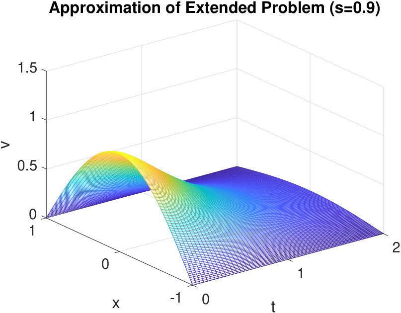 Figure 1
Peer Reviews
No public reviews on file for this paper yet. If you reviewed it on a platform where reviews are public (OpenReview, ICLR, NeurIPS, ICML), you can paste yours below so the community can read it here.
Videos
No videos yet. Explain this paper in a talk, walkthrough, or lecture? Add one.
Analysis of an approximation to a fractional extension problem
Joshua L. Padgett
Department of Mathematics and Statistics, Texas Tech University, Broadway and Boston, Lubbock, TX 79409-1042
Abstract
The purpose of this article is to study an approximation to an abstract Bessel-type problem, which is a generalization of the extension problem associated with fractional powers of the Laplace operator. Motivated by the success of such approaches in the analysis of time-stepping methods for abstract Cauchy problems, we adopt a similar framework herein. The proposed method differs from many standard techniques, as we approximate the true solution to the abstract problem, rather than solve an associated discrete problem. The numerical method is shown to be consistent, stable, and convergent in an appropriate Banach space. These results are built upon well understood results from semigroup theory. Numerical experiments are provided to demonstrate the theoretical results.
keywords:
Fractional diffusion , Nonlocal operators , Singular equations , Degenerate equations , Bessel equations , Semigroup methods
1 Introduction
Due to its wide array of applications, the computation of fractional powers of the Laplacian, and other elliptic operators, has become a problem of great interest [2, 9, 25, 26]. Fractional powers of operators have received this attention due to their applicability to the accurate modeling of real-world problems with varying scales. Examples of such problems are found in porous media flow, peridynamics, nonlocal continuum field theory, finance, and many others (see [8, 10, 13, 29], and the references therein). However, due to the nonlocal nature of fractional problems, the development of accurate and efficient computational algorithms has been greatly hindered. In response to this hurdle, the revolutionary work by Caffarelli and Silvestre demonstrated that the nonlocal fractional Laplacian problem may be recast into an equivalent local problem which is amenable to certain standard numerical techniques [7].
In order to demonstrate, fix and consider the function which solves
[TABLE]
where is a given function of appropriate regularity and the fractional power of the Laplacian is defined via the hypersingular integral
[TABLE]
with being some normalization constant [7]. Caffarelli and Silvestre then showed that for the fractional Laplacian in can be realized via the Dirichlet-to-Neumann map for a function The function then satisfies the following Bessel-type equation
[TABLE]
where is the solution to Moreover, the function satisfying may be viewed as the harmonic extension of to the fractional dimension One can then calculate as
[TABLE]
where is a constant depending upon but not on the dimension and solves Moreover, the final equality is is known as the conormal derivative. We have emphasized the relationship between and in in order to clarify the ensuing exposition. Further details and applications of this method may be found in [3, 7, 14, 31].
Several numerical algorithms for solving problems involving fractional powers of the Laplacian have been developed based upon the Caffarelli-Silvestre extension technique [12, 18, 25, 26]. These methods have also been extended to problems involving general elliptic operators and various other physically relevant nonlocal problems. Despite the increased interest in such methods, these explorations are still in their infancy and merit further consideration. Moreover, there is the need to improve the efficiency and accuracy of existing numerical methods.
In order to develop more robust approximations to we consider the following abstract Bessel-type problem
[TABLE]
where is a real separable Banach space, is a densely defined linear operator, and There have been numerous studies concerned with approximating particular forms of but herein we present a novel method and demonstrate its properties in an arbitrary Banach space for appropriate abstract operators In particular, such analysis allows for mesh independent results, which are quite useful in application.
Analysis and representations of the true solution of have been studied in multiple settings [3, 14, 31]. However, to the author’s knowledge, approximations to in this abstract setting have yet to be explored. In particular, the true solution to involves the abstract semigroup generated by the operator and there have been few methods employing direct approximations of this operator. These approximations preserve numerous desirable properties inherent to the original semigroup operator, often resulting in superior approximations, resulting in qualitatively superior approximations [6, 15, 27, 28].
This article is organized as follows. In Section 2 relevant mathematical preliminaries are outlined for the reader’s convenience. Section 3 is concerned with the development and stability of the proposed approximation to Section 4 provides the necessary results to guarantee convergence of the proposed method. Section 5 presents some concrete example of our abstract problem and provides numerical experiments verifying the analytic result. Finally, concluding remarks and an outline of future endeavors are given in Section 6.
2 Preliminaries
Let be a real separable Banach space with norm denoted and let denote the Banach algebra of bounded operators on We wish to consider the following Bessel-type problem
[TABLE]
where and is linear. The operator norm on will also be denoted by Before providing details regarding a solution to we detail a necessary assumption and some relevant background.
Assumption 1**.**
Let the operator be closed and densely defined in Moreover, let be strictly dissipative in
We recall that an operator is called strictly dissipative if and only if
[TABLE]
and it is called strictly dissipative if and only if it satisfies the additional range condition
[TABLE]
The notion of a dissipative operator may also be formalized in the following manner. Define the (left) semi-inner-product on the Banach space as
[TABLE]
Then is strictly dissipative if and only if
[TABLE]
Note that the limit in exists as is a G-differential of the norm If is a Hilbert space then we have that coincides with the true inner product on that is Moreover, we have that for any and
[TABLE]
for any More details regarding properties of may be found in [11].
Remark 2.1*.*
It is worth noting that many existing works in the direction of abstract numerical analysis often require that an operator simply be m-dissipative. The current work requires a slightly stricter result in order to guarantee the appropriate decay of the solution (a requirement similar to that in [14, 25]).
From this, it readily follows that the resolvent operator of a strictly dissipative operator is well-defined and a contraction in It also follows that strictly dissipative operators generate strongly continuous semigroups of contractions [16, 21]. We will denote the semigroup generated by by Note that if is reflexive then every strictly dissipative operator is densely defined. More details regarding dissipative operators and their properties can be found in [4, 21].
The following example demonstrates that standard elliptic operators are examples of the proposed abstract formulation.
Example 2.1**.**
Let be a bounded domain with smooth boundary. We may then consider the operator with homogeneous Dirichlet boundary conditions, on Let and for we define
[TABLE]
We then have, by employing integration by parts and standard Sobolev-type inequalities, that
[TABLE]
where is some positive constant. Thus, we have that for all The range condition follows from standard results, as well.
We also define the logarithmic norm of an operator with respect to the semi-inner-product given by to be
[TABLE]
Logarithmic norms have been well studied and more details regarding their properties may be found in [30].
Example 2.2**.**
If we consider the situation in Example 2.1, again, then it is easy to see that where
Remark 2.2*.*
It is worth noting that one could easily have considered (the negation) of any strongly elliptic operator in Examples 2.1 and 2.2, not just the Laplacian. In fact, one could equivalently define strongly elliptic operators as any operator such that
Remark 2.3*.*
While not the focus of this work, one may easily use to define the notion of ellipticity of nonlinear operators on This approach can be quite useful and allows for the consideration of more generalized notions of numerical stability for stiff systems of equations.
The above formulations allow us to develop the following, very useful, result.
Lemma 2.1**.**
Let be the generator of a strongly continuous semigroup in Then,
[TABLE]
Proof.
This result has been proven elsewhere, but we include a proof for completeness. Let be the generator of the semigroup Then it follows that is the solution to
[TABLE]
Recall that the upper right Dini derivative of a function is defined as
[TABLE]
By direct calculation, we have
[TABLE]
(see, for instance, [11]). Employing and solving directly yields the desired result.
The remainder of this section will serve as a brief introduction to fractional powers of operators in Banach spaces and provide some existence results for problem . These introductory notes are based primarily on the reference [22], with some influence from [23]. Let denote the set of all bounded linear operators mapping into and
[TABLE]
denote the resolvent set of the linear operator For operators satisfying Assumption 2.1 and we define the Balakrishnan operator with power and base as
[TABLE]
This operator will be used to define fractional powers of the operator For more details see [22].
Remark 2.4*.*
The operator inherits numerous desirable properties from the underlying operator For instance, if is bounded or injective, then so is [22].
With we are now able to define fractional powers of abstract operators.
Definition 2.1**.**
Let be as in Assumption 2.1 and fix Then we define as
- i.
for
- ii.
for being unbounded.
- iii.
for being unbounded, (where is the spectrum of ), and given by
[TABLE]
It is worth noting that the above definition yields a well-defined closed operator which extends the original Balakrishnan operator. Moreover, in [23], it was shown that for a densely defined linear operator we have
[TABLE]
There is still a wealth of information that one could present to provide background on fractional powers of operators, but these ideas will not be pertinent to the study at hand. Interested readers should see [22] for more details.
Based on Assumption 2.1, we are in fact considering a special case of that studied in [14]. Though the following result was included in [14], the proof was omitted for this special case, hence, we include a proof for completeness. The methods employed below are similar to those in [23].
Theorem 2.1**.**
Let Then a solution to is given by
[TABLE]
and also satisfies
[TABLE]
where
Proof.
We first show by demonstrating directly that satisfies for To that end we have
[TABLE]
and
[TABLE]
Thus, for we have
[TABLE]
By noting that and employing integration by parts, we have
[TABLE]
which shows that is a solution to
Next we show holds for Note that
[TABLE]
By employing integration by parts in we obtain
[TABLE]
where the boundary terms in go to zero due to Assumption 2.1. After substituting into and employing integration by parts yet again, we obtain
[TABLE]
Note that the first integral in is Bochner integrable and is in fact the desired result, as
[TABLE]
by Definition 2.1 and Thus, follows if the second integral in goes to zero. By Taylor expanding T(z) about and employing Assumption 2.1, we have
[TABLE]
Since it follows that is bounded by assumption and we have
[TABLE]
Combining and yields the desired result.
Lemma 2.2**.**
For all a solution to is given by
Proof.
This result follows from [23] and the fact that is densely defined in
It is worth noting that the solution to is not known to be unique in the current setting. However, there are numerous results regarding situations in which uniqueness is known, for instance, when is the Laplacian with Dirichlet boundary conditions, when is a sectorial operator and is a Hilbert space, and for all operators when [3, 14, 23, 31]. In order to avoid these issues in our ensuing analysis, we introduce the following assumption.
Assumption 2**.**
The solution to is unique in for all and hence, given by
Remark 2.5*.*
One could replace Assumption 2.2 with the condition that the solution to decays to zero at infinity, in some weak sense, and obtained the same result.
Remark 2.6*.*
It is worth noting that may seem a bit strange as it involves the fractional power of the operator However, as discussed in the Introduction, when considering or in applications the function will be given.
We close this section by outlining some basic properties regarding the semigroup generated by and the operator For more details, see [17].
Lemma 2.3**.**
Let and Then there exists a constant such that
- i.
* for *
- ii.
* on *
- iii.
If then
3 Derivation of Approximation
The properties of various forms of have been studied by several authors, see [3, 14, 23, 31] and the references therein. However, in this paper, we are concerned with the development and analysis of an approximation to To that end, fix with Then we define and set For the sake of the ensuing analysis, we define
[TABLE]
We then have the following result.
Lemma 3.1**.**
Let and be defined as in and respectively. Then, if we have
[TABLE]
where is a constant independent of and
Proof.
We proceed by direct calculation. We have
[TABLE]
where by Assumption 2.1 and is defined in It now remains to bound the integral in To that end, let to obtain
[TABLE]
Employing the substitution in then yields
[TABLE]
where
[TABLE]
Since we have
[TABLE]
By substituting - into we obtain
[TABLE]
Remark 3.1*.*
While the constant, in Lemma 3.1 is independent of and it does depend on Hence, in practice, if is close to zero we will need to increase the value of to obtain the desired accuracy.
Now that it has been established that the truncation of the integral will not have drastic effects on the approximation of for large we present the proposed approximation to in For we define the following continuous in time approximation to
[TABLE]
where
[TABLE]
with
Assumption 3**.**
Let the operator be nonexpansive in
Remark 3.2*.*
Note that if is in fact a Hilbert space, then the assumption that is nonexpansive will always be valid due to Assumption 2.1. That is, let then
[TABLE]
where is the inner product on the Hilbert space However, in general Assumption 3.1 does not hold in general Banach spaces, with satisfying Assumption 2.1. For more details see [4].
We begin by demonstrating that is stable in
Lemma 3.2**.**
Let and be as defined in Then we have
[TABLE]
where is a constant independent of and
Proof.
Direct calculation yields
[TABLE]
by Assumption 3.1. Thus it we need only consider the We first note that since for we have
[TABLE]
for some Now let be the index such that We then have, by
[TABLE]
By noting that
[TABLE]
we then obtain
[TABLE]
where is a constant independent of and Substituting into completes the proof.
4 Convergence
We now present several convergence estimates that will be necessary for the main result of this section.
Lemma 4.1**.**
Let Then we have
[TABLE]
for where is a constant independent of and
Proof.
We begin by defining
[TABLE]
for all Thus, by employing we have by direct calculation
[TABLE]
for some By noting that
[TABLE]
it is clear from that it only remains to show
[TABLE]
for We first note that, by Hille’s theorem, we have
[TABLE]
From Assumption 2.1, and Lemma 2.3, we have
[TABLE]
since is bounded for and
We next note that
[TABLE]
Combining and into then yields
[TABLE]
where for respectively, and is a constant independent of and
We now define a family of operators which will be employed in the proof of the following lemma. Let be defined as
[TABLE]
with The satisfy the following recurrence relation
[TABLE]
Lemma 4.2**.**
Let Then we have
[TABLE]
where is a constant independent of and
Proof.
By employing and we readily obtain
[TABLE]
for Further, consideration of gives
[TABLE]
Combining and finally gives
[TABLE]
The result for then follows by taking the norm of both sides of Since is a bounded operator on it follows that holds for and taking the norm of both sides yields the result for
Combining the above results, we have the following theorem demonstrating the desired convergence rate of the proposed scheme.
Theorem 4.1**.**
Let Then, we have
[TABLE]
where is a constant independent of and
Proof.
We begin by writing the difference as follows
[TABLE]
We will now apply the previous lemmas to and First, by Lemma 3.1, it is immediately clear that we have
[TABLE]
and thus may be made arbitrarily small for large enough Next, by Lemma 4.1 we have
[TABLE]
where the value of changes throughout the calculations, but remains independent of and with or depending on the regularity of the initial data. Finally, by Lemma 4.2, Assumption 2.1, and Assumption 3.1, we have
[TABLE]
where, once again, is independent of and with as before. Combining the obtained bounds in - yields the desired result.
Remark 4.1*.*
The first term in our estimate
[TABLE]
is an expected and standard term (a similar term appears in, for example, [5, 9]). However, we intend to remove this estimate in future work by relating the choice of to the parameter
5 Numerical Experiments
In order to further verify the sharpness of our analysis and demonstrate the efficacy of the proposed method, we present some numerical experiments. The first and second examples consider a one-dimensional and two-dimensional problem, respectively, where the given operator is the Laplace operator. In both cases, we see that the expected theoretical convergence results are recovered. The third example outlines how our theory easily includes general strongly elliptic differential operators which still satisfy the theoretical results from Theorem 4.1.
It is the case that the nonlocality of fractional problems can increase memory requirements to the point that some standard methods become quite inefficient. To that end, we briefly explore the memory requirements needed to implement the proposed method If we fix a particular numerical approximation of the operator then our method can be shown to be Initially, it may seem that the computations are more involved, due to the evaluation of the operator (seeming to require additions and multiplications), but these evaluations can be be completed with only additions and multiplications by employing nested operations similar to the classical Horner algorithm for polynomials. To determine an exact efficiency, one must consider the precise discretization method employed to approximate the operator Due to the inversion needed to compute it is clear that discretizations resulting in a banded matrix structure will prove the most efficient. We leave more detailed studies of the efficiency, as well as computational run time trials, for future work.
5.1 A One-Dimensional Example
Let and define with its usual inner product and norm. Consider the problem
[TABLE]
where
[TABLE]
and the fractional Laplacian is defined via the spectral definition (which can be done due to the smoothness of ). That is,
[TABLE]
where the set forms an orthonormal basis of and satisfy
[TABLE]
for each and
[TABLE]
where is the usual inner product on The true solution to can be found explicitly and is given by
[TABLE]
This true solution may be obtained by using We will first demonstrate how our method can approximate problems such as by taking the trace of and then consider the convergence properties of the approximation of the solution to the extension problem given by
As has been demonstrated in this work, it is the case that can be recovered from the following extension problem:
[TABLE]
where and In order to implement the problem, we replace the operator with some finite dimensional discretization. For simplicity, we employ the standard second-order finite difference method on uniform grids [19]. It is worth noting that the use of any other consistent spatial disretization method is acceptable, and as seen below, the convergence rate in the spatial direction will not be affected. The freedom to choose the discretization method for the operator is one of the primary benefits of this approach.
The tables in Fig. 5.1 demonstrate the numerical convergence rates of the scheme given by For these experiments, we chose a modest value of in order to demonstrate the efficacy of the method with respect to the truncation. It is clear from this table that the numerical solution converges at the expected rates given by Theorem 4.1. For the sake of clarity, we present a plot of the numerical solution to in Fig. 5.2.
Finally, we finish this example by presenting convergence rates for several other choices of the parameter These results are presented in Fig. 5.3 and further verify our theoretical results. For brevity, we omit the convergence rates for the parameter as they are not affected by these choices and match those of Fig. 5.1.
Remark 5.1*.*
We wish to note that our experiments have shown that more modest choices of may still provide accurate numerical solutions, as well. However, we leave a more detailed study of these choices for future endeavors.
Remark 5.2*.*
We also wish to note that one could potentially increase efficiency of the proposed numerical method by allowing it to be run in parallel. For instance, one may rewrite the method as
[TABLE]
where
[TABLE]
While the implementation of requires more direct evaluations than the original algorithm, one can easily compute in parallel by noting that
[TABLE]
While there is a slight decrease in accuracy due to employing it is the case that for complicated operators this could potentially be a favorable trade-off.
5.2 A Two-Dimensional Example
Let We then once again consider the problem but with
[TABLE]
where are the first eigenpair of the operator on and are given by
[TABLE]
and
[TABLE]
where is the first Bessel function of the first kind, is the first zero of and and are real-valued constants that ensure
By using one may determine the true solution of the extension problem to be given by
[TABLE]
where is the modified Bessel function of the second kind (see [1] for more information regarding the aforementioned Bessel functions and their properties). Moreover, it can be shown that
Just as before, we discretize the operator using standard finite differences (see, for example, [20] for more details on doing so for as above). However, in this example we will only consider convergence aspects of the method in the extended variable direction. A table with convergence rates for various choices of the parameter are given in Fig. 5.4. As before, the results are in agreement with the rates given in Theorem 4.1.
5.3 A General Second-Order Elliptic Operator
As should be clear from the outlined theory, the proposed numerical algorithm will still be applicable when the operator is a general strongly elliptic operator on some domain Following the construction developed in [9], let be given by
[TABLE]
where (here we emphasize the difference between the variable and the extended variable, ). We assume that the function with almost everywhere, is symmetric and positive definite, and that is sufficiently smooth. Then, it follows that given there exists a unique such that
[TABLE]
Moreover, we have that satisfies Assumption 2.1. It is clear that the operator’s domain is densely defined in If we employ the same framework as that in Example 2.1, then we have
[TABLE]
where is the standard inner product on is a positive constant, and the final inequality follows from the fact that is positive definite and is positive almost everywhere. Thus, we have for all as desired. Further, the range condition of a strictly dissipative operator is satisfied, as well. Thus, it follows that our approximation, given by of the Bessel-type problem
[TABLE]
is well-defined, stable, and convergent. Moreover, it follows that the initial datum, will be the solution of the following nonlocal elliptic problem
[TABLE]
It should be noted that we have omitted some more technical details, such as the fact that the operator may be extended to the fractional space since such things are not relevant to the current discussion (this is because we are considering functions with higher regularity to guarantee the theoretical rates of convergence). However, interested readers may see [14], and the reference therein, for more details.
In order to provide an explicit example, we let and Since we do not have an explicit solution to on hand, we will approximate the numerical rate of convergence. Let denote the numerical solution obtained by on a grid defined by the parameter Then we define to be the numerical solution obtained by on a grid with spacing We then have the following Milne device for determining the numerical rate of convergence, denoted given by
[TABLE]
where the differences are defined on the grid associated to (the least refined grid) and the norm is an appropriately chosen norm (in our case, the discrete norm).
Remark 5.3*.*
The convergence of the numerical method given by is also influenced by the error of truncating domain of the Bessel-type problem. However, by assuming this error is roughly constant, which is reasonable for a fixed value of and the approximation given by will be accurate.
The table in Fig. 5.5 demonstrates the obtained numerical convergence rates for various choices of with We see from the table that the computed values still reflect the expected theoretical values obtained in Theorem 4.1. Moreover, we present the convergence rate for the case when to verify the expected second-order convergence of our method.
6 Concluding Remarks
In this article, we consider an approximation to an abstract extension problem, that is the generalization of the method demonstrated by Caffarelli and Silvestre in [7]. This generalized setting allows for the consideration of a wider class of problems, while also allowing for the use of robust nonlinear functional analytic techniques. By taking this novel approach, we develop methods which differ from those presented in [9, 12, 18, 25], yet are quite effective. In particular, this approach allows for the consideration of semigroup theory within the numerical framework. As such, the method is able to exhibit favorable qualities.
Herein, we provide an approach where we approximate the true solution to the extended problem, as compared to the standard approach of discretizing the underlying system first. The approximation is shown to be stable, consistent, and convergent for appropriately smooth initial data. Moreoever, the employed Padé approximation allows for the efficient construction of the numerical solution via factorization techniques. However, one could easily replace this approximation with any desired second-order (or higher) approximation to the associated abstract Cauchy problem.
Moving forward, we will consider improved approximations methods within the same abstract framework. In particular, we will consider abstract analysis of higher-order Padé approximations and quadrature techniques, including Runge-Kutta and exponential integration methods, with the goal of constructing methods of arbitrary order. This will also allow for the consideration of the underlying algebraic structures of these methods, as has been done with Butcher and Lie-Butcher series for classical problems [24]. We also intend to extend these results to abstract problems posed on abstract manifold structures, allowing for the consideration of novel problems in differential geometry. Moreover, we hope to better understand how well this extension technique preserves and approximates the Dirichlet-to-Neumann map that is of fundamental importance in the underlying theory. Preliminary work indicates that our proposed numerical method faithfully represents this operator after applying the conormal derivative given by , but there is still a need to finish developing a rigorous analysis of this application. However, more immediate concerns will be the deeper comparison of our newly proposed methods with popular existing methods for the fractional Laplacian problem.
Acknowledgements
This work was supported by the NSF grant number 1903450. The author would like to thank Akif Ibraguimov, of Texas Tech University, for introducing this problem to them. The author is also thankful for Akif’s time and insightful suggestions that greatly improved the quality of the work herein. Finally, the author is thankful to the reviewers who provided numerous useful suggestions that greatly improved the presentation of the numerical experiments in Section 5.
The reference list from the paper itself. Each links out to its DOI / PubMed record.
- 1[1] M. Abramowitz and I. A. Stegun. Handbook of mathematical functions: with formulas, graphs, and mathematical tables , volume 55. Courier Corporation, 1965.
- 2[2] H. Antil and E. Otárola. A FEM for an optimal control problem of fractional powers of elliptic operators. SIAM Journal on Control and Optimization , 53(6):3432–3456, 2015.
- 3[3] W. Arendt, A. F. M. Ter Elst, and M. Warma. Fractional powers of sectorial operators via the Dirichlet-to-Neumann operator. Communications in Partial Differential Equations , 43(1):1–24, 2018.
- 4[4] V. Barbu. Nonlinear differential equations of monotone types in Banach spaces . Springer Science & Business Media, 2010.
- 5[5] A. Bonito, W. Lei, and J. E. Pasciak. Numerical approximation of the integral fractional Laplacian. Numerische Mathematik , 142(2):235–278, 2019.
- 6[6] C. J. Budd and A. Iserles. Geometric integration: numerical solution of differential equations on manifolds. Philosophical Transactions of the Royal Society of London A: Mathematical, Physical and Engineering Sciences , 357(1754):945–956, 1999.
- 7[7] L. Caffarelli and L. Silvestre. An extension problem related to the fractional Laplacian. Communications in Partial Differential Equations , 32(8):1245–1260, 2007.
- 8[8] P. Carr, H. Geman, D. B. Madan, and M. Yor. The fine structure of asset returns: An empirical investigation. The Journal of Business , 75(2):305–332, 2002.