A combinatorial identity with applications to forest graphs
Tony C. Dorlas, Alexei L. Rebenko, Baptiste Savoie

TL;DR
This paper presents an elementary proof of a combinatorial identity relevant to graph theory and demonstrates its applications in counting forests with explicit formulas.
Contribution
It introduces a new combinatorial identity and applies it to derive closed-form enumeration formulas for forests.
Findings
Elementary proof of a combinatorial identity
Closed-form enumeration formulas for forests
Applications in graph theory enumeration
Abstract
We give an elementary proof of an interesting combinatorial identity which is of particular interest in graph theory and its applications. Two applications to enumeration of forests with closed-form expressions are given.
Click any figure to enlarge with its caption.
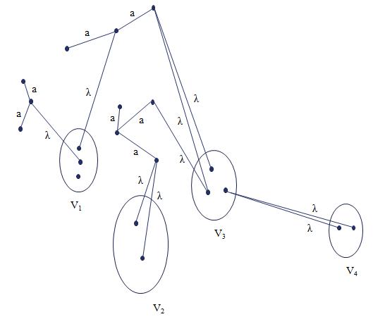 Figure 1
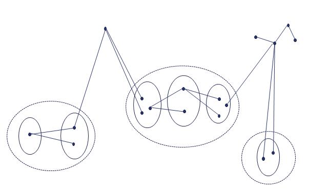 Figure 2
Peer Reviews
No public reviews on file for this paper yet. If you reviewed it on a platform where reviews are public (OpenReview, ICLR, NeurIPS, ICML), you can paste yours below so the community can read it here.
Videos
No videos yet. Explain this paper in a talk, walkthrough, or lecture? Add one.
A combinatorial identity with applications to forest graphs.
Tony Dorlas Dublin Institute for Advanced Studies, School of Theoretical Physics, Dublin, Ireland
Alexei Rebenko Institute of Mathematics, Ukrainian National Academy of Sciences, Kyiv, Ukraine
Baptiste Savoie11footnotemark: 1 , Corresponding author - e-mail: [email protected]
Abstract
We give an elementary proof of an interesting combinatorial identity which is of particular interest in graph theory and its applications. Two applications to enumeration of forests with closed-form expressions are given.
The aim of this paper is to give a new, elementary proof of the combinatorial identity (1) in Theorem 1 and give some non-trivial applications to enumeration of forests. Done by induction, the proof we give is simple in that it only requires the use of the binomial formula along with the derivation operator. This identity finds an interest in graph theory (for enumeration of forests) and its applications. For instance, we came across (1) when evaluating, within the framework of rigorous statistical mechanics, contributions from forest graphs to a cluster expansion for classical gas correlation functions in [2]. Other applications of such rooted graphs in theoretical physics are for example in the works [5, 6, 3, 4]. The combinatorial identity (1) provides a means to directly derive a closed-form expression for the number of distinct rooted forests on a fixed collection of sets of vertices, see formula (2) in Theorem 2. A more complicated situation involving additional vertices with different weighting factors is also treated, see formula (3) in Theorem 3. The identity (1) is in fact known: see [10], Theorem 5.3.4, Equation (5.47). However, it is formulated and proved there in terms of forest graphs, and thereby not easily recognizable. Here we present a direct and self-contained proof. We also note that formula (1) is similar to Hurwitz’ generalization of Abel’s formula, see, e.g., [1, 8, 9].
1 The combinatorial identity.
Theorem 1**.**
Given with , and a collection of (complex) numbers , the following identity holds
[TABLE]
where the sum on the left-hand side is over the set of all partitions of into non-empty subsets.
The proof of Theorem 1 is postponed to Sec. 3.
2 Two applications to enumeration of forests.
A rooted (or directed) forest is defined on a collection of sets of vertices as a graph on with connected components which are trees, such that there are no lines between vertices of any individual , and moreover, if each set is reduced to a single point and lines eminating from it to a single line, then the graph reduces to a single (connected) tree. Further, if in the reduced tree, () is connected to in the path from to , then all lines between and eminate from a single vertex in (a root). This definition may appear complicated, but in fact in many situations such directed forests occur naturally. See, e.g., [5, 6, 3, 4, 2, 9]. Deriving a closed-form expression for the number of (distinct) forests as described above becomes straightforward by using Theorem 1. Note that a direct proof of Theorem 2 was given in [2].
Theorem 2**.**
Given , the number of distinct forests on a collection of sets of vertices is given by
[TABLE]
Proof.
Set
[TABLE]
For we can choose the root in ways and connect it to points in . This results in different forests (in fact, disregarding isolated vertices, they are trees). Suppose now that the statement is true for . Considering a forest on sets of vertices, the vertices of can be connected to other sets in the reduced tree on . Omitting the connections to we obtain separate forests given by subsets of . If contains , then this yields a factor
[TABLE]
the additional factor being due to the choice of root for the connection to . Similarly, the other branches yield factors
[TABLE]
The resulting expression for is
[TABLE]
Identity (1) yields
[TABLE]
This concludes the proof of Theorem 2.
Another, more complicated application is considered in Theorem 3 below. We refer the readers to Figure 1 in Sec. 4.2 for an illustration of a generic configuration.
Theorem 3**.**
Given , let be a collection of sets of vertices and let be additional single vertices. Define a quantity as follows. Every forest on gives a contribution to defined by positive constants and such that every edge between two additional vertices and contributes a factor whereas all other edges contribute a factor . Then
[TABLE]
where and , .
Proof.
We proceed by induction on . For , the contributions to are given by a number of separate trees, each connected to a vertex of . The number of trees on a subset of the additional vertices is , each contributing a factor since is the number of edges in the tree, and there is an additional factor due to the choice of vertex connecting to a point of . Hence
[TABLE]
For we define to be the contribution of forests such that there is no edge between vertices of different sets . We claim that
[TABLE]
Assuming this, we can complete the induction. Indeed, we can subdivide the set into subsets such that the with are connected. These forests contribute factors of the form
[TABLE]
where is the first vertex in and . This is analogous to the first application, see Theorem 2. The sets can now be considered as single sets in a reduced forest (except that an additional vertex is connected to a single , i.e. is replaced by ). Denote by the corresponding contribution. By the claim (4), this contribution equals
[TABLE]
Summing over the subdivisions yields
[TABLE]
Identity (3) then follows by summing over . To conclude the proof of Theorem 3, it remains to show (4). The proof essentially relies on the rewriting of in the form
[TABLE]
Here, denotes the set of ordered -tuples in where each pair is unequal, i.e.
[TABLE]
The expression (4) then follows from the following version of the multinomial formula:
[TABLE]
For reader’s convenience, the proof of (5) is postponed to Sec. 4.1.
3 Proof of Theorem 1.
The proof is done by induction on and . Note that, for both sides are equal to 1 and for both sides are equal to . Now assume that identity (1) holds true for a given and all . Let and denote the left-hand side and right-hand side of (1) respectively. We may assume that and expand the factor by the binomial formula in powers of
[TABLE]
Inserting this into and denoting , we have
[TABLE]
If , we separate out , for which . If then . Conversely, given a partition we obtain a unique partition of by adding to any of the sets with . We can therefore write
[TABLE]
Note that in the second term on the right-hand side, since . Expanding the quantity (the right-hand side of (1) but with ) in powers of and then replacing by , it follows that it suffices to prove the equivalent identities
[TABLE]
for , and
[TABLE]
for all . We start with the case of . By the induction hypothesis, the first term on the left-hand side of (6) is equal to
[TABLE]
The second term on the left-hand side of (6) can be rewritten as
[TABLE]
again by the induction hypothesis. Adding the two contributions for yields the right-hand side of (6). For the case , the left-hand side of (7) can simply be rewritten as
[TABLE]
Next, we prove the case where . The key idea is to apply the derivation operator to the left-hand side of (1). This gives
[TABLE]
The term on the right-hand side of (8) is equal to zero unless . In that case,
[TABLE]
independently of . Hence, the left-hand side of (8) can be rewritten as
[TABLE]
which is nothing but times the left-hand side of (7). On the other hand, applying the derivation operator to the right-hand side of (1) gives
[TABLE]
which is just times the right-hand side of (7). This concludes the proof of (7), and hence also the proof of the theorem.
4 Appendix.
4.1 Proof of (5).
Proof.
We proceed by induction on . For , formula (4) gives
[TABLE]
which reduces to (4) by Theorem 1 since .
For , consider first the case that all are already connected by trees. Denote by the contribution to due to forest graphs where is connected to a single subset . We have by induction that this contribution to is given by
[TABLE]
Here, the first term in curly brackets corresponds to the case where is connected to the same tree as , and the second term corresponds to the case where is connected to for some by a separate tree. Note that factors in (5) correspond to trees connected to a single .
For the first term in curly brackets we set and define () if and , and for the second term we put and and . Then is a subdivision of and we can write
[TABLE]
Next, consider the case where there are two groups of ( resp. ) which are connected by trees among themselves but not between each other. Then and have to be connected via . A similar configuration is illustrated in Figure 2 placed in Sec. 4.2. If then can be connected to in two ways: directly to one of the trees on or by a separate tree to one of the vertices of . By induction we therefore have that
[TABLE]
Note that if then we set in which case the sums over and are absent as well as the first term in curly brackets. Now, for the first term in curly brackets, we put , for and and , and for . This defines a subdivision of where the subset containing has at least two elements. Similarly, for the second term we put and for and , and for . This is also a subdivision of , where in this case . Conversely, suppose that is a subdivision of . Let be the set containing . Consider first the case where for all . Then we define the subdivision with for and and choose an arbitrary subdivision of . We can assume and define for and for , and set and . The sum over subdivisions then reduces to
[TABLE]
where we used Theorem 1 with for and .
The other extreme is when for all . In that case we have and . Only the second term applies and we remove from the list to obtain a subdivision of , where . There are now two cases: either and for , or . Again choosing a subdivision of , we assume and set if and for , and otherwise and , and for and for . In the latter case and . The sum over subdivisions becomes
[TABLE]
In the general case we can have either or . If , this corresponds to the first term in curly brackets and we define the subdivision with for and and choose an arbitrary subdivision of . We can assume . Then we set and . If then we eliminate and set and . In both cases, the sum over subdivisions then reduces to
[TABLE]
where we used Theorem 1 with for and . We conclude that
[TABLE]
It is now clear that the case where there are more groups , of subsets connected via is analogous. We again consider the set containing and distinguish the cases where is equal to or greater than 1. We map to subdivisions in the same way as in case and obtain a factor
[TABLE]
The result is
[TABLE]
Finally, summing over yields (5).
4.2 Some illustrations.
Acknowledgment.
The authors thank Adrien Kassel for having brought to their attention reference [10]. The authors also thank Benjamin Hackl for having brought to their attention his paper [7] related to our main result Theorem 1. The second author gratefully acknowledges the financial support of the Ukrainian Scientific Project ”III-12-16 Research of models of mathematical physics describing deterministic and stochastic processes in complex systems of natural science”.
The reference list from the paper itself. Each links out to its DOI / PubMed record.
- 1[1] N. H. Abel, Beweis eines Ausdrucks, von welchem die Binomial-Formel ein einzelner Fall ist , J. Reine Angew. Math. 1 , 159–160 (1826)
- 2[2] T.C. Dorlas, A.L. Rebenko and B. Savoie, Correlation of clusters: Partially truncated correlation functions and their decay , J. Math. Phys. 61 , 033303 (2020)
- 3[3] M. Duneau, D. Iagolnitzer and B. Souillard, Strong cluster properties for classical systems with finite-range interaction , Commun. Math. Phys. 35 (4), 307–320 (1974)
- 4[4] M. Duneau and B. Souillard, Cluster properties of lattice and continuous systems , Commun. Math. Phys. 47 , 155–166 (1976).
- 5[5] G. Gallavotti and F. Nicolo, Renormalization theory in four-dimensional scalar fields. I , Commun. Math. Phys. 100 (4), 545–590 (1985)
- 6[6] G. Gallavotti and F. Nicolo, Renormalization theory in four-dimensional scalar fields. II , Commun. Math. Phys. 101 (2), 247–282 (1985)
- 7[7] B. Hackl, A combinatorial identity for rooted labeled forests , Aequationes Math. 94 , 253–257 (2020)
- 8[8] A. Hurwitz, Uber Abel’s Verallgemeinerung der binomischen Formel , Acta Math. 26 , 199–203 (1902)