Equivalence of regression curves sharing common parameters
Kathrin M\"ollenhoff, Frank Bretz, Holger Dette

TL;DR
This paper introduces a bootstrap test for comparing two regression curves sharing common parameters, demonstrating its effectiveness through theory, simulations, and a clinical trial example.
Contribution
It develops a new bootstrap test for assessing the similarity of regression curves with shared parameters, improving power over traditional methods.
Findings
Test controls level effectively
Achieves higher power with shared parameters
Validated through simulation and clinical trial example
Abstract
In clinical trials the comparison of two different populations is a frequently addressed problem. Non-linear (parametric) regression models are commonly used to describe the relationship between covariates as the dose and a response variable in the two groups. In some situations it is reasonable to assume some model parameters to be the same, for instance the placebo effect or the maximum treatment effect. In this paper we develop a (parametric) bootstrap test to establish the similarity of two regression curves sharing some common parameters. We show by theoretical arguments and by means of a simulation study that the new test controls its level and achieves a reasonable power. Moreover, it is demonstrated that under the assumption of common parameters a considerable more powerful test can be constructed compared to the test which does not use this assumption. Finally, we illustrate…
Click any figure to enlarge with its caption.
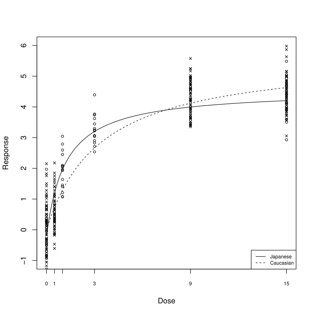 Figure 1
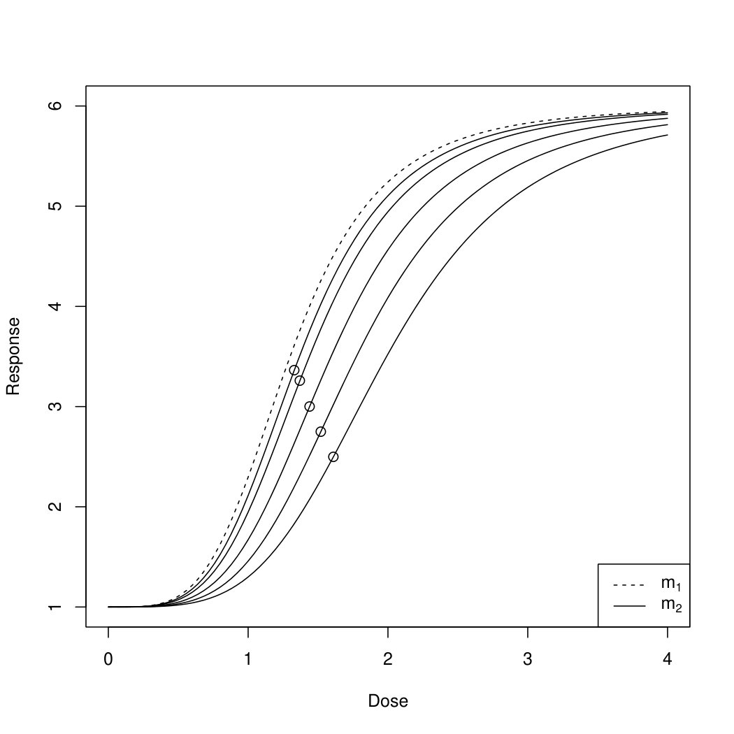 Figure 2
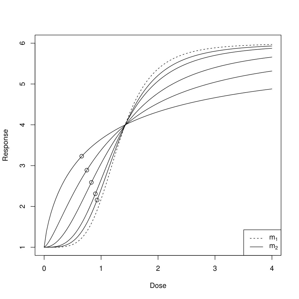 Figure 3
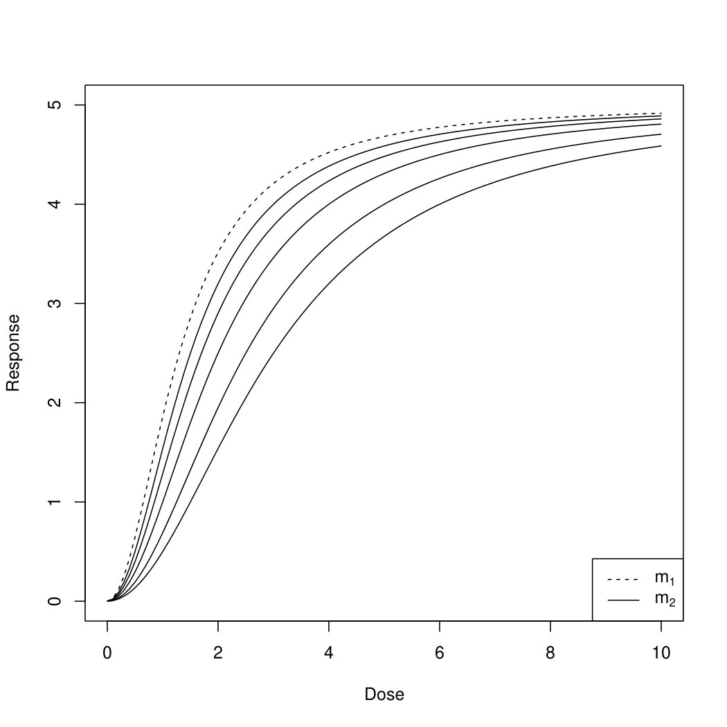 Figure 4
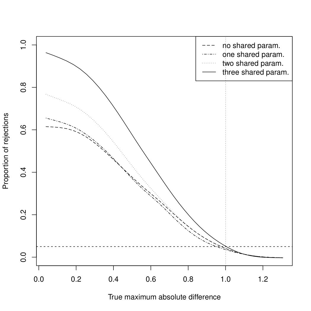 Figure 5
| 2 | 0.002 (0.000) | 0.010 (0.005) | 0.012 (0.009) | 0.002 (0.004) | 0.018 (0.013) | 0.031 (0.019) | |
|---|---|---|---|---|---|---|---|
| 1.5 | 0.014 (0.013) | 0.035 (0.028) | 0.027 (0.043) | 0.026 (0.020) | 0.055 (0.049) | 0.052 (0.070) | |
| 1 | 0.068 (0.058) | 0.054 (0.065) | 0.051 (0.060) | 0.106 (0.099) | 0.109 (0.114) | 0.115 (0.121) | |
| 2 | 0.000 (0.000) | 0.000 (0.000) | 0.001 (0.002) | 0.000 (0.000) | 0.000 (0.000) | 0.002 (0.002) | |
| 1.5 | 0.004 (0.001) | 0.010 (0.006) | 0.013 (0.015) | 0.005 (0.005) | 0.021 (0.014) | 0.026 (0.020) | |
| 1 | 0.048 (0.071) | 0.053 (0.043) | 0.062 (0.059) | 0.104 (0.122) | 0.101 (0.097) | 0.129 (0.117) | |
| 2 | 0.000 (0.000) | 0.000 (0.000) | 0.000 (0.000) | 0.000 (0.000) | 0.000 (0.000) | 0.000 (0.004) | |
| 1.5 | 0.000 (0.000) | 0.003 (0.000) | 0.002 (0.000) | 0.002 (0.000) | 0.011 (0.002) | 0.012 (0.009) | |
| 1 | 0.056 (0.061) | 0.040 (0.061) | 0.042 (0.063) | 0.103 (0.102) | 0.090 (0.102) | 0.096 (0.109) | |
| 1 | 0.288 (0.263) | 0.091 (0.062) | 0.493 | 0.125 (0.108) | 0.114 (0.106) | |
|---|---|---|---|---|---|---|
| 2 | 0.389 (0.358) | 0.118 (0.090) | 0.739 | 0.174 (0.157) | 0.172 (0.148) | |
| 3 | 0.460 (0.427) | 0.134 (0.105) | 0.841 | 0.228 (0.198) | 0.211 (0.185) | |
| 1 | 0.166 (0.152) | 0.054 (0.036) | 0.184 | 0.067 (0.064) | 0.063 (0.061) | |
| 2 | 0.237 (0.219) | 0.076 (0.054) | 0.355 | 0.107 (0.086) | 0.091 (0.086) | |
| 3 | 0.280 (0.261) | 0.091 (0.062) | 0.450 | 0.130 (0.112) | 0.113 (0.105) | |
| 1 | 0.123 (0.115) | 0.040 (0.029) | 0.129 | 0.050 (0.057) | 0.049 (0.046) | |
| 2 | 0.171 (0.170) | 0.057 (0.041) | 0.241 | 0.073 (0.072) | 0.068 (0.063) | |
| 3 | 0.219 (0.204) | 0.070 (0.050) | 0.322 | 0.095 (0.086) | 0.091 (0.084) |
| 0.5 | 0.137 (0.154) | 0.075 (0.078) | 0.070 (0.073) | 0.238 (0.266) | 0.172 (0.155) | 0.137 (0.145) | |
|---|---|---|---|---|---|---|---|
| 0.25 | 0.208 (0.190) | 0.102 (0.101) | 0.081 (0.088) | 0.344 (0.349) | 0.196 (0.188) | 0.152 (0.170) | |
| 0 | 0.181 (0.203) | 0.105 (0.105) | 0.086 (0.092) | 0.333 (0.361) | 0.196 (0.213) | 0.154 (0.154) | |
| 0.5 | 0.341 (0.424) | 0.180 (0.230) | 0.132 (0.153) | 0.505 (0.581) | 0.311 (0.357) | 0.246 (0.279) | |
| 0.25 | 0.550 (0.675) | 0.249 (0.315) | 0.166 (0.190) | 0.733 (0.802) | 0.428 (0.484) | 0.305 (0.348) | |
| 0 | 0.664 (0.783) | 0.286 (0.353) | 0.191 (0.188) | 0.822 (0.884) | 0.463 (0.562) | 0.338 (0.367) | |
| 0.5 | 0.481 (0.593) | 0.297 (0.359) | 0.207 (0.273) | 0.635 (0.729) | 0.460 (0.502) | 0.355 (0.406) | |
| 0.25 | 0.826 (0.868) | 0.448 (0.569) | 0.280 (0.357) | 0.902 (0.933) | 0.635 (0.719) | 0.477 (0.545) | |
| 0 | 0.917 (0.961) | 0.559 (0.665) | 0.342 (0.415) | 0.966 (0.989) | 0.740 (0.812) | 0.520 (0.596) | |
| 2 | 0.002 (0.000) | 0.001 (0.000) | 0.001 (0.000) | 0.000 (0.005) | 0.003 (0.007) | 0.006 (0.011) | |
|---|---|---|---|---|---|---|---|
| 1.5 | 0.000 (0.001) | 0.003 (0.000) | 0.008 (0.001) | 0.007 (0.033) | 0.002 (0.030) | 0.016 (0.054) | |
| 1 | 0.036 (0.035) | 0.044 (0.040) | 0.053 (0.039) | 0.083 (0.099) | 0.110 (0.116) | 0.113 (0.112) | |
| 2 | 0.000 (0.000) | 0.000 (0.000) | 0.000 (0.000) | 0.000 (0.000) | 0.000 (0.002) | 0.004 (0.002) | |
| 1.5 | 0.000 (0.000) | 0.000 (0.000) | 0.004 (0.000) | 0.000 (0.007) | 0.004 (0.021) | 0.012 (0.022) | |
| 1 | 0.052 (0.057) | 0.028 (0.040) | 0.016 (0.036) | 0.104 (0.113) | 0.068 (0.117) | 0.056 (0.105) | |
| 2 | 0.000 (0.000) | 0.000 (0.000) | 0.000 (0.000) | 0.000 (0.000) | 0.000 (0.000) | 0.000 (0.000) | |
| 1.5 | 0.000 (0.000) | 0.000 (0.000) | 0.004 (0.000) | 0.000 (0.000) | 0.000 (0.004) | 0.004 (0.004) | |
| 1 | 0.056 (0.032) | 0.036 (0.036) | 0.040 (0.036) | 0.100 (0.088) | 0.080 (0.100) | 0.076 (0.088) | |
| 0.5 | 0.130 (0.147) | 0.096 (0.075) | 0.094 (0.072) | 0.231 (0.245) | 0.191 (0.133) | 0.174 (0.125) | |
|---|---|---|---|---|---|---|---|
| 0.25 | 0.156 (0.194) | 0.102 (0.089) | 0.087 (0.085) | 0.275 (0.319) | 0.197 (0.178) | 0.157 (0.147) | |
| 0 | 0.155 (0.164) | 0.108 (0.076) | 0.087 (0.059) | 0.310 (0.316) | 0.197 (0.166) | 0.189 (0.137) | |
| 0.5 | 0.312 (0.542) | 0.124 (0.225) | 0.140 (0.133) | 0.528 (0.697) | 0.240 (0.384) | 0.260 (0.240) | |
| 0.25 | 0.384 (0.689) | 0.224 (0.289) | 0.164 (0.173) | 0.560 (0.841) | 0.396 (0.484) | 0.292 (0.313) | |
| 0 | 0.448 (0.663) | 0.192 (0.259) | 0.148 (0.163) | 0.616 (0.807) | 0.372 (0.455) | 0.240 (0.309) | |
| 0.5 | 0.528 (0.780) | 0.220 (0.392) | 0.160 (0.228) | 0.688 (0.896) | 0.404 (0.632) | 0.256 (0.400) | |
| 0.25 | 0.724 (0.904) | 0.320 (0.544) | 0.260 (0.304) | 0.824 (0.936) | 0.540 (0.740) | 0.408 (0.516) | |
| 0 | 0.644 (0.920) | 0.308 (0.580) | 0.224 (0.248) | 0.800 (0.956) | 0.532 (0.728) | 0.404 (0.484) | |
Peer Reviews
No public reviews on file for this paper yet. If you reviewed it on a platform where reviews are public (OpenReview, ICLR, NeurIPS, ICML), you can paste yours below so the community can read it here.
Videos
No videos yet. Explain this paper in a talk, walkthrough, or lecture? Add one.
Equivalence of regression curves sharing common parameters
Kathrin Möllenhoff1, Frank Bretz2 , Holger Dette1
1 Department of Mathematics, Ruhr-Universität Bochum, Germany,
2Novartis Pharma AG, CH-4002 Basel, Switzerland
Abstract
In clinical trials the comparison of two different populations is a frequently addressed problem. Non-linear (parametric) regression models are commonly used to describe the relationship between covariates as the dose and a response variable in the two groups. In some situations it is reasonable to assume some model parameters to be the same, for instance the placebo effect or the maximum treatment effect. In this paper we develop a (parametric) bootstrap test to establish the similarity of two regression curves sharing some common parameters. We show by theoretical arguments and by means of a simulation study that the new test controls its level and achieves a reasonable power. Moreover, it is demonstrated that under the assumption of common parameters a considerable more powerful test can be constructed compared to the test which does not use this assumption. Finally, we illustrate potential applications of the new methodology by a clinical trial example.
Keywords and Phrases: Similarity of regression curves, equivalence testing, parametric bootstrap, nonlinear regression, dose finding studies
1 Introduction
Regression models are commonly used to describe the relationship between multiple covariates and a response variable. In certain applications, more than one regression model is available, such as when assessing the relationship between the covariates and the response variables in more than one population (e.g. in males and females). It is then often of interest to demonstrate the equivalence of the regression curves: If equivalence can be claimed, conclusions can be drawn from the pooled sample and a single regression model is sufficient to describe the data. This can be achieved by testing a suitable null hypothesis that the distance between the regression curves (measured in an appropriate sense) is smaller than a pre-specified equivalence margin at a controlled Type I error rate. Note that the problem of equivalence testing, as considered in this paper, is conceptually different from the more frequent problem of testing for equality of curves and is much less studied in the literature due to methodological difficulties.
The problem of testing for equality of regression models has been intensively discussed in the nonparametric context and we refer to the recent work of Feng et al., (2015), whichcontains a rather comprehensive list of references. In applied regression analysis, however, parametric models are usually preferred to a purely nonparametric approach as they admit a direct interpretation of the observed effects in terms of the model parameters. In addition, the available information of the observations is increased by applying more efficient estimation or test procedures, provided that the assumed model is valid. Despite its importance, the problem of establishing equivalence of two parametric regression models while controlling the Type I error rate has only recently found attention in the literature. Using the intersection-union test device from Berger, (1982), Liu et al., (2009) investigated the assessment of non-superiority, non-inferiority and equivalence when comparing two regression models over a restricted covariate region. Building upon this work, Gsteiger et al., (2011) derived equivalence tests based on simultaneous confidence bands for nonlinear regression models, with application to population pharmacokinetic analyses. Likewise, Bretz et al., (2016) assessed the similarity of dose response curves in two non-overlapping subgroups of patients. Alternatively, Dette et al., (2018) suggested directly estimating the distance between the regression curves and using a non-standard bootstrap test to decide for equivalence of the two curves if the estimate is less than a certain threshold. Expanding this approach, Moellenhoff et al., (2018) assessed the comparability of drug dissolution profiles via maximum deviation, whereas Hoffelder, (2018) demonstrated the equivalence of dissolution profiles using the Mahalanobis distance; see also Collignon et al., (2018).
In these papers, the authors assumed that the regression models have different parameters and can therefore be evaluated separately. In some applications, however, this assumption cannot be justified and it is more reasonable to assume that the regression models may have some common parameters. The total number of parameters to estimate is then reduced to the common and remaining parameters of each model, affecting the asymptotic behavior of the estimators. Consider, for example, the Phase II dose finding trial for a weight loss drug described in Bretz et al., (2016). This trial aimed at comparing the dose response relationship for two regimens administered to patients suffering from overweight or obesity: Three doses each for once daily (o.d.) and twice daily (b.i.d.) use of the medication, and placebo. It is reasonable to assume that the placebo response is the same under both the o.d. and the b.i.d. regimen. Since the regression models typically used for dose response modeling contain a parameter for the placebo response (Pinheiro et al., (2006)), they will thus share this common parameter for both the o.d. and the b.i.d. regimen. In some instances, it might even be reasonable to assume that the maximum efficacy for high doses is similar in both groups. Moreover, clinical trial sponsors may even decide to use the same placebo group for logistical reasons. The response of each patient on placebo is then used twice in the estimation of the o.d. and b.i.d. dose response models, further complicating the statistical problem.
In this paper, we investigate the equivalence of two parametric regression curves that share common parameters. In Section 2 we first introduce the regression models to be estimated under the assumption of common parameters. We then develop a non-standard bootstrap test which performs the resampling under the constraints of the interval hypotheses implied by the equivalence test problem. The new tests improves the procedure proposed in Dette et al., (2018) using the additional information of common parameter in both groups. We also discuss testing the equivalence of model parameters to assess whether the assumption of common parameters is plausible. In Section 3 we investigate the finite sample properties of the proposed bootstrap test proposed in terms of power and size. In Section 4 we illustrate the methods using a multi-regional clinical trial example where it is conceivable that the placebo and maximum treatment responses are the same across geographic regions but the onset of treatment differs due to intrinsic and extrinsic factors (Malinowski et al., (2008); ICH, (2017)). Technical details and proofs are deferred to an appendix.
2 Methodology
2.1 Models with common parameters
Let
[TABLE]
denote the observed response of the th subject at the th dose level under the th dose response model , where denotes the index of the two groups under consideration. We assume that the (non-linear) regression model is parametrized through a -dimensional vector , . Note that the regression models and may be different. Likewise, the parameters and may be different even if . We further assume that the error terms are independent and identically distributed with expectation [math] and variance . The dose levels may be different in both groups but they are attained on the same (restricted) covariate region . In this paper is assumed to be the dose range, although the results can be generalized to include other covariates. Further, denotes the sample size in group where we assume observations in the th dose level (. The sample sizes can be unequal and the total number of observations is denoted by .
In this paper we consider the situation, where the regression models have some common parameters. More precisely, we assume without loss of generality that these parameters are given by the first model parameters of the parameter in model (2.1) that is
[TABLE]
where denotes the vector of common parameters in both regression models and and denote the remaining parameters in the models and , respectively, which do not necessarily coincide. The case where the models and do not share any common parameters is included and corresponds to for (that is ). As a consequence the -dimensional vector of all parameters of the regression functions in model (2.1) under the assumption (2.2) is given by . Throughout this paper we assume that where is a compact set.
These parameters are now estimated by least squares using the combined sample , that is
[TABLE]
2.2 Testing equivalence of regression curves
Following Liu et al., (2009) and Gsteiger et al., (2011) we consider the regression curves and to be equivalent if the maximum distance between the two curves is smaller than a given pre-specified constant, say , that is,
[TABLE]
In clinical trial practice is often referred to as a relevance threshold in the sense that if the difference between the two curves is believed not to be clinically relevant. In order to establish equivalence of the two curves and at a controlled type I error, we will develop a test for the hypotheses
[TABLE]
In the following we extend the bootstrap approach from Dette et al., (2018) to test the hypotheses (2.4) in the situation of common parameters. Note that the test procedure proposed below could also be applied to alternative measures of equivalence, such as the integrated deviation .
Algorithm 2.1**.**
(parametric bootstrap for testing equivalence under the assumption of common parameters)
- (1)
Calculate the ordinary least-square (OLS) parameter estimate (2.3) assuming a common parameter . The corresponding variance estimates are given by
[TABLE]
where . Calculate the estimate
[TABLE]
for the maximal deviation between the two regression curves.
- (2)
Define the constrained estimates
[TABLE]
where minimize the objective function in (2.3) under the additional restriction
[TABLE]
Define and note that .
The next two steps describe the (parametric) bootstrap procedure.
- (3)
Generate data
[TABLE]
with independent and normally distributed errors .
- (4)
Calculate the OLS estimate as in Step (1) and the test statistic
[TABLE]
where . The quantile of the distribution of the distribution of the statistic is denoted by and the null hypotheses in (2.4) is rejected, whenever
[TABLE]
In practice the can be calculated repeating steps (3) and (4), say times, in order to obtain replicates of . An estimate of then is defined by , where denotes the corresponding order statistic, and this estimate is used in (2.9) **
The following theorem states that this algorithm yields a valid test procedure. The proof is left to the Appendix 6.
Theorem 2.1**.**
The test defined by (2.9) is a consistent, asymptotic -level test. That is
[TABLE]
whenever , and
[TABLE]
if .
Remark 2.2**.**
The results presented in this section remain correct in trials with a common placebo group, where observations are taken at dose level (corresponding to placebo), which are modelled by the random variables . For the sake of a simple presentation we consider location-scale type models, such that the common effect at the placebo can easily be modelled, but we note that more general models can be considered as well introducing additional constraints for the parameter.
To be precise, we assume that the models in (2.1) are given by
[TABLE]
where , such that the condition reflects the fact that there is only one placebo group (and as a consequence a common placebo parameter). Models of this type cover the most frequently used functional forms used in drug development and several examples can be found in Ting, (2006). Beside the location parameter there may be also other shared parameters, which we do not reflect in our notations for a better readability. The -th model is completely characterized by its parameter , , and we obtain estimates of the model parameters by minimizing the sum of squares
[TABLE]
Theorem 2.1 remains valid in this situation and a proof can be found in the Appendix (see Section 6.4). **
2.3 Testing equivalence of model parameters
So far we assumed that the two regression models and share the common parameter . In practice it may be necessary to assess whether this assumption is plausible using an appropriate equivalence test for the shared model parameters. To be more precise, we recall the definition the parameters in model (2.1), i.e.
[TABLE]
and note that assumption (2.2) of common parameters in the models and can be represented as for . In order to investigate if this assumption holds at least approximately we construct a test for the hypotheses
[TABLE]
where denotes the equivalence margin. To be precise let denote the least squares estimates in model for the sample (), and assume that for large sample considerations the sample sizes and converge to infinity such that
[TABLE]
Under standard assumptions, which are listed in Section 6 it can be shown that the least squares estimate of the parameter in model is approximately normal distributed, that is
[TABLE]
where the symbol means convergence in distribution and the matrix is defined by
[TABLE]
Here and throughout this paper we assume that the matrices and are non-singular. Consequently the difference is also asymptotically normal distributed, and in particular it follows for the first components of the difference that
[TABLE]
where the matrix is defined by
[TABLE]
\Lambda_{\ell}^{-1}=\big{(}(\Sigma_{\ell}^{-1})_{ij})\big{)}_{i,j=1}^{p^{\prime}} denotes the upper-left -block of the matrix and is defined in (2.16). Therefore we obtain the approximation
[TABLE]
where is defined in (2.20). We can now apply the test proposed in Wang et al., (1999) by rejecting the null hypothesis in (2.14), whenever
[TABLE]
where denotes the quantile of the -distribution with degrees of freedom and the th diagonal element of the matrix which is an estimate for the (unknown) covariance matrix (this is obtained by replacing the unknown parameters , and weights in (2.18) by their corresponding estimates and , respectively).
3 Finite sample properties
We now investigate the finite sample properties of the bootstrap test proposed in Section 2.2 in terms of power and size using numerical simulations. The data is generated as follows:
- (a)
We choose the functional form of the models and specify their parameters (including a common parameter ), which determine the true underlying models. Further we choose variances and the actual dose levels , . 2. (b)
For each dose we calculate values for the response given by . By generating residual errors we obtain the final response data
[TABLE]
The simulation results below were obtained using simulation runs, where bootstrap replications were used to calculate quantiles of the bootstrap test.
In the following, we report the simulations results for power and size under three different scenarios. We consider the four-parameter sigmoid Emax model
[TABLE]
which is frequently used in practice when modeling dose response relationships (see for example Gabrielsson and Weiner, (2007) or Thomas et al., (2014)). In model (3.2) the parameter corresponds (in this order) to the placebo effect , the maximum effect , the Hill parameter determining the steepness of the dose-response curve and the dose producing half of the maximum effect (Macdougall, (2006)). In what follows we add an index for a shared parameter or for the group under consideration.
Scenario 1: We assume the dose range with identical dose levels , for both regression models . For each configuration of we use (3.1) to simulate observations at each dose level , resulting in total sample sizes of , respectively. We first compare the two sigmoid Emax models
[TABLE]
assuming the shared parameters . The only difference between the two models is in the parameters and , which results in the need to estimate five parameters in total. We consider the reference sigmoid Emax model with the parameters and . This reference model is compared to various specifications of the second model determined by , , , , , and common shared parameters . The values for were chosen such that the maximum absolute distances are given by , , , , , [math] respectively. For these are attained at the dose levels and ; see Figure 1. For , that is , the maximum distance is attained at every point in .
In Table 1 we summarize the simulated rejection probabilities of the bootstrap test (2.9) under the null hypothesis (2.4) with and . We conclude that the bootstrap test controls its level in all cases under consideration. At the margin of the null hypothesis (i.e. ) the approximation of the level is very precise, even for sample sizes as small as .
We also investigated the relative residual mean squared errors (RRMSE) of the parameters estimates. Table 2 summarizes the simulation results only for (i.e. at the margin of the null hypothesis), as the results are similar for other choices of . We conclude that the RRMSE for estimating the Hill parameter is (by far) the largest. This phenomenon has also been observed by Mielke, (2016). We also observe that all estimation errors decrease with larger sample sizes and smaller variances. Table 2 also summarizes the RRMSE when fixing the Hill parameter at (see the numbers in brackets). In this case, four parameters need to be estimated in total and the estimation errors become slightly smaller. We also repeated the Type I error rate simulations when fixing the Hill parameter at . The the results are reported in Table 1 (numbers in brackets) and we conclude that the size is well controlled within the simulation error.
In Table 3 we summarize the power of the bootstrap when generating the data under the alternative and . As expected, the power increases with larger sample sizes and smaller variances and is reasonably high across all configurations. Fixing the Hill parameter significantly improves the power which can be explained by the difficulty of estimating this parameter precisely, as discussed above.
Scenario 2: We maintain the basic settings from Scenario . We consider again two sigmoid Emax models
[TABLE]
but assume now that both, the placebo response and the maximum treatment effect , are the same. For the reference model we chose , and . We investigated the maximum distances , which resulted in the following parameter configurations for the second model:
[TABLE]
The maximum distances between the two curves are now attained at the dose levels and ; see Figure 1.
In Table 4 we summarize the simulated rejection probabilities under the null hypothesis (2.4) for and . We conclude again that the bootstrap test controls the designated significance level in all cases under consideration. Especially at the margin the simulated Type I error rates are close to the nominal level . These observations apply regardless of whether the Hill parameter is estimated or fixed at the true underlying values given in (3).
In Table 5 we summarize the simulated power of the bootstrap test under the alternative and . As expected, the power decreases for increasing values of and for higher variances or smaller sample sizes. One noticeable exception occurs at , where in some cases the power is smaller than for . This effect can be explained theoretically when considering the proofs for the bootstrap test. In case of the set containing all points where the maximum distance between the two curves is attained (see Appendix 6.3) consists of the entire dose range . Therefore, the asymptotic distribution of the test statistic is not Gaussian but a maximum of Gaussian processes. This complex structure of the asymptotic distribution has an impact on the bootstrap procedure and explains the decrease in power for . This phenomenon can also be observed, although to a lesser degree, in Scenario . Finally, we observe higher power values when fixing the Hill parameter compared to the situation where it has to be estimated.
Scenario 3: We now investigate the operating characteristics of the bootstrap test assuming three, two, one and no shared parameters. We set , and compare again two sigmoid Emax models. The true placebo response is chosen as . The reference model is specified by . The second model is specified by , where is chosen such that the maximum distances with respect to lie between [math] and ; see the resulting curves plotted in Figure 2 for . Consequently the parameters specifying the two models only differ in parameters and and the maximum distance is determined by the choice of . As all other parameters are the same for the two models, we can compare the bootstrap test assuming three, two, one and no shared parameter. Note that we do not consider the case of identical models (i.e. ) because of the discontinuity of power at described under Scenario 2. The dose range is given by with different dose levels , , , , . We create observations at each dose level for each group according to (3.1), which results in a total sample size of . Finally, we choose , .
In Figure 2 we plot the proportion of rejections in dependence of the true maximum absolute difference . Under the null hypothesis all four tests control their level, as the proportion of rejections is smaller than or equal to within simulation errors. Looking at the region , we observe that the test assuming three shared parameters has the highest power among all four tests, followed by the test assuming two shared parameters. The difference between the tests assuming one and no shared parameter is rather small. Concluding, the more parameters can be assumed to be common for the two regression curves the higher is the power of the test. Note, however, that strictly speaking the hypotheses (2.4) are different when assuming three, two, one and no shared parameters and that the perceived power gain when assuming more shared parameters comes at the cost of making additional assumptions that need to be verified in practice, as illustrated with the clinical trial example in Section 4.
4 Clinical trial example
We now illustrate the proposed method with a multi-regional clinical trial example. The objective of this trial is to evaluate the dose response relationships in Caucasian and Japanese patients and assess their similarity. Based on data from previous clinical trials investigating a drug with a similar mode of action, it is reasonable to assume a similar response to placebo and a common maximum treatment effect in both populations, with the main difference expected to be in a different onset of treatment effect. Using the sigmoid Emax model (3.2), these consideration thus lead to different and Hill parameters for the two dose response curves. Because the trial is still at its design stage, we simulate data based on the trial assumptions. To maintain confidentiality, we scale the actual doses to lie within the [0, 15] interval. These limitations do not change the utility of the calculations below.
We assume Japanese and Caucasian patients, resulting in patients overall. Patients from both populations are randomized to receive either placebo (dose level [math]) or one of three active dose levels, namely for the Japanese and and for the Caucasian patients. Assuming equal allocation of patients within each population, we thus have 75, 60, 15, 15, 60, and 75 patients randomized to the dose levels and , respectively. The response variable is assumed to be normally distributed and larger values indicate a better outcome. Pharmacological and clinical considerations suggest the use of the (three-parameter) Emax model with the Hill parameter fixed at 1. Later on we relax this assumption as part of a sensitivity analysis. The R code for this example and all other calculations in this paper is available from the authors upon request.
In Figure 3 we display the fitted dose response models and for the Japanese and Caucasian patients, respectively, together with the individual observations, where and the -axis is truncated to for better readability. The parameter estimates from the two separate model fits are given by and . The observed differences for the placebo response and the maximum treatment effect are given by and , respectively, and thus relatively small, as it also transpires from the plots in Figure 3. To corroborate this empirical observation, we formally test whether the assumption of shared parameters is plausible by applying the equivalence test described in Section 2.3 on the data set under consideration. We choose the threshold and therefore test the null hypothesis against the alternative Applying the test (2.21) for , we obtain and and therefore \delta-t_{1-\alpha,n-2}\big{(}\tfrac{\hat{\Omega}_{11}}{n(n-2)}\big{)}^{1/2}=1.191 and \delta-t_{1-\alpha,n-2}\big{(}\tfrac{\hat{\Omega}_{22}}{n(n-2)}\big{)}^{1/2}=0.928, respectively. We can thus reject at the relatively stringent 5% level and conclude equivalence of the two parameters, which justifies using the bootstrap test (2.1) with shared parameters.
We now evaluate the similarity of the dose response curves for the Japanese and Caucasian patients, assuming the same placebo and maximum treatment effect. In order to compute the non-linear least squares estimates in model (2.1) with (2.2) we formulate the objective function of the minimization step as
[TABLE]
Here, denotes the (shared) placebo effect, the (shared) maximum treatment effect , and and the parameters of the two models. Using the auglag function from the alabama package Varadhan, (2014) to solve the above optimization problem, we obtain the parameter estimates , , and . In brackets we report the associated standard errors, which have to be calculated manually based on (5.5). The estimates for the population variances are and . The observed maximum difference between both curves over the investigated dose range is , attained at dose . We apply the bootstrap test (2.9) using bootstrap replications. Setting for the equivalence margin in (2.4), we obtain the quantile for . Thus, we reject the null hypothesis (2.4) at the 5% significance level and conclude that the dose response curves for the Japanese and Caucasian populations are similar, under the shared parameter assumption. Alternatively, we can calculate the -value for the bootstrap test and obtain the same test decision at level . For illustration purposes we also apply the bootstrap test (2.9) but without shared parameters (yet under the assumption of a fixed Hill parameter). Accordingly, we obtain a considerably larger -value of , which supports our findings from Scenario in Section 3 about the loss in power when no shared parameters are assumed. In this case the observed maximum distance is , attained at dose , and the quantile of the bootstrap distribution is .
Finally, we perform a sensitivity analysis to investigate the assumption of the Hill parameter being equal to 1. As part of this analysis we repeat the model fit and the bootstrap test using the sigmoid Emax model (3.2) where the Hill parameter is now part of the estimation. The parameter estimates (standard errors in brackets) are , , , , and . Now, the maximum distance between the curves is , attained at dose . It turns out that the standard errors of the estimates are slightly higher which is in line with the results shown in the simulation studies in Section 3. Performing again the bootstrap test with two shared parameters results the quantile and the -value . Consequently, we cannot reject the null hypothesis in this case. In conclusion, fixing the Hill parameter to 1 and assuming both the placebo effect and the maximum treatment effect to be the same in both populations clearly results in the most powerful procedure. We can demonstrate equivalence at the significance level of , whereas in case of estimating both models separately (i.e. no shared parameters) or including the Hill parameter in the estimation we obtain considerably larger -values.
5 Conclusion
In this paper we developed a new test for the equivalence of two regression curves when it is reasonable to assume that some model parameters are the same. Our approach is based on an estimate of the maximum deviation between the two curves, where critical values are obtained by a novel constraint bootstrap procedure. We demonstrated that the new test controls its level properly and is consistent.
We investigated the finite sample properties of the proposed procedure using extensive simulations and observed that the Type I error rate is controlled in all scenarios under consideration, even for sample sizes as small as patients per dose level. Further, we concluded that the test reaches a reasonable power that increases with larger sample sizes. In particular, we demonstrated that the power of tests for the equivalence of curves can be improved substantially by using the additional information of common parameters in the two regression curves. This effect could also be observed in the clinical trial example, which showed the power advantage of the bootstrap test (2.9) if the underlying assumptions are well justified. Relaxing those assumptions may lead to more robust conclusions, but only at a cost of a loss in power.
An interesting extension of the proposed methodology arises from the need to include covariates in clinical trial practice. Covariates can be continuous (e.g. age or body mass index), categorical (e.g. disease status or race), or binary (e.g. gender or smoking yes/no), possibly changing over time. These cases may have to be treated differently and we leave this problem for future research. Another area of research could be the assessment of similarity in two nested populations, thus relaxing the assumption of independence between the observations. In our multi-regional clinical trial example we compared the Japanese with Caucasian patients. It will be interesting and relevant to clinical trials to explore the development of the proposed methods when comparing the Japanese with an overall population that includes Japanese and Caucasian patients. Again, we leave this topic for future research.
Acknowledgments This work has been supported in part by the Collaborative Research Center “Statistical modeling of nonlinear dynamic processes” (SFB 823, Teilprojekt T1) of the German Research Foundation (DFG) Parts of this manuscript were written while Frank Bretz was on a sabbatical leave at University of Canterbury in Christchurch, New Zealand. He would like to thank Dr. Daniel Gerhard for his support.
6 Appendix: Proof of Theorem 2.1 and Remark 2.2
The proof of the theoretical results of this paper proceeds in several steps. First we state the assumptions under which the statements hold (Section 6.1). Second, we derive the asymptotic distribution of the parameter estimates in models with common parameters (Section 6.2). In Section 6.3 we derive a result on the weak convergence of a stochastic process, from which the proof of Theorem 2.1 and Remark 2.2 can be derived (see Section 6.4).
6.1 Assumptions
For the theoretical results of this paper we make the same assumptions as in Dette et al., (2018).
The errors are independent, have finite variance and expectation zero. 2. 2.
The covariate region is compact and the number and location of dose levels does not depend on . 3. 3.
All estimates of the parameters are computed over compact sets and . 4. 4.
The regression functions and are twice continuously differentiable with respect to the parameters for all in neighbourhoods of the true parameters and all . The functions and their first two derivatives are continuous on . 5. 5.
The gradients with respect to the parameters are uniformly bounded, that is
6. 6.
Defining we assume that for any there exists a constant such that
[TABLE]
6.2 Asymptotic properties of the OLS
In this section we derive the asymptotic normality of the parameter estimates in models with common parameters. Observing the definition of the OLS in (2.3) we obtain, by taking the partial derivatives, by the necessary conditions
[TABLE]
Defining
[TABLE]
for we can write
[TABLE]
where denotes the zero vector in . Therefore the equations in (5.1) can be summarized to
[TABLE]
A Taylor expansion now yields
[TABLE]
and therefore can be linearized as
[TABLE]
Due to the strong law of large numbers it holds
[TABLE]
where the matrices and are defined by
[TABLE]
respectively. Therefore, using the representation in (5.3) and the result in (5.4) we obtain the asymptotic normality of the estimate, that is
[TABLE]
6.3 Weak convergence of a stochastic process
The essential step in the proof is a result regarding the weak convergence of the process
[TABLE]
We further define which yields
Proof.
At first we derive a linearization of by using the Taylor expansion \tilde{\Delta}(d,\hat{\beta})=\tilde{\Delta}(d,\beta)+\big{(}\tfrac{\partial\tilde{\Delta}(d,\beta)}{\partial\beta}\big{)}^{T}(\hat{\beta}-\beta)^{T}+R(\beta), where is a remainder term and due to (5.3) we have . Therefore it holds \sqrt{n}\tilde{p}_{n}(d)=\sqrt{n}\big{(}\tfrac{\partial\tilde{\Delta}(d,\beta)}{\partial\beta}\big{)}^{T}(\hat{\beta}-\beta)^{T}+o_{\mathbb{P}}(1) uniformly with respect to (note that due to the assumptions is continuous in and is a compact set) and with the result from (5.3) this can be written as
[TABLE]
Observing (5.3) we define
[TABLE]
and obtain
[TABLE]
We now define f(d):=\big{(}\tfrac{\partial\tilde{\Delta}(d,\beta)}{\partial\beta}\big{)}^{T}\Sigma^{-1/2}, and we consider the map
[TABLE]
Obviously, using the same arguments as before, is continuous and therefore the same holds for . Consequently, (5.5) and the Continuous Mapping Theorem (see for example van der Vaart, (2000)[p.7 f.]) yield
[TABLE]
uniformly with respect to , where , which proves the assertion. ∎
6.4 Proof of Theorem 2.1 and Remark 2.2
The assertion of Theorem 2.1 now follows by the same arguments as given in the proof of Theorem 4 in Dette et al., (2018). In particular it can be shown that
[TABLE]
where denote the sets of extremal points, that is those points, where the unknown difference attains it maximum absolute deviation. The details are omitted for the sake of brevity.
Similarly, note that in the situation of a common placebo group as described in Remark 2.2 the estimates are obtained by minimizing the sum of squares in (2.13). As , , this function is the same as the one which is obtained allocating the observations at placebo arbitrarily to the two groups. More precisely, we can also write the sum of squares in (2.13) as
[TABLE]
where () and (). This corresponds to the minimzation of the sum of squares in (2.3) with a common intercept , and consequently this situation can be treated in the same way as considering two different placebo groups with a common intercept . By the same arguments as given in Appendix 6.2 the corresponding estimates are asymptotically normal distributed (if and for some constants ), and the proof in Section 6.3 shows that Theorem 2.1 remains valid in the model with a common placebo group. As a consequence we obtain the claim in Remark 2.2
The reference list from the paper itself. Each links out to its DOI / PubMed record.
- 1Berger, (1982) Berger, R. L. (1982). Multiparameter hypothesis testing and acceptance sampling. Technometrics , 24:295–300.
- 2Bretz et al., (2016) Bretz, F., M. K., Dette, H., Liu, W., and Trampisch, M. (2016). Assessing the similarity of dose response and target doses in two non-overlapping subgroups. ar Xiv:1607.05424 .
- 3Collignon et al., (2018) Collignon, O., Moellenhoff, K., and Dette, H. (2018). Equivalence analyses of dissolution profiles with the mahalanobis distance: a regulatory perspective and a comparison with a parametric maximum deviation-based approach. Biometrical Journal .
- 4Dette et al., (2018) Dette, H., Möllenhoff, K., Volgushev, S., and Bretz, F. (2018). Equivalence of regression curves. Journal of the American Statistical Association , 113:711–729.
- 5Feng et al., (2015) Feng, L., Zou, C., Wang, Z., and Zhu, L. (2015). Robust comparison of regression curves. TEST , 24(1):185–204.
- 6Gabrielsson and Weiner, (2007) Gabrielsson, J. and Weiner, D. (2007). Pharmacokinetic and Pharmacodynamic Data Analysis: Concepts and Applications . Swedish Pharmaceutical Press, Stockholm, 4th edition.
- 7Gsteiger et al., (2011) Gsteiger, S., Bretz, F., and Liu, W. (2011). Simultaneous confidence bands for nonlinear regression models with application to population pharmacokinetic analyses. Journal of Biopharmaceutical Statistics , 21(4):708–725.
- 8Hoffelder, (2018) Hoffelder, T. (2018). Equivalence analyses of dissolution profiles with the mahalanobis distance. Biometrical Journal .