The application of the Lattice Boltzmann method to the one-dimensional blood flow dynamics in elastic vessels
Oleg Ilyin

TL;DR
This paper demonstrates that the Lattice Boltzmann method can effectively model one-dimensional blood flow in elastic vessels, capturing nonlinear wave propagation and vessel stiffening with high accuracy.
Contribution
It introduces a Lattice Boltzmann model for blood flow in elastic vessels, linking kinetic theory with cardiovascular dynamics, and validates it through various test problems.
Findings
Accurate modeling of nonlinear wave propagation in elastic vessels
Effective simulation of artery stiffening effects
Good agreement with previous results in test cases
Abstract
The one-dimensional nonlinear equations for the blood flow motion in distensible vessels are considered using the kinetic approach. It is shown that the Lattice Boltzmann (LB) model for non-ideal gas is asymptotically equivalent to the blood flow equations for compliant vessels at the limit of low Knudsen numbers. The equations of state for non-ideal gas are transformed to the pressure-luminal area response. This property allows to model arbitrary pressure-luminal area relations. Several test problems are considered: the propagation of a sole nonlinear wave in an elastic vessel, the propagation of a pulse wave in a vessel with varying mechanical properties (artery stiffening) and in an artery bifurcation, in the last problem Resistor-Capacitor-Resistor (RCR) boundary conditions are considered. The comparison with the previous results show a good precision.
Click any figure to enlarge with its caption.
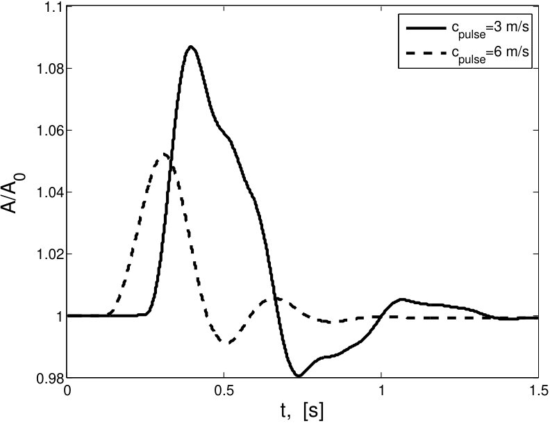 Figure 1
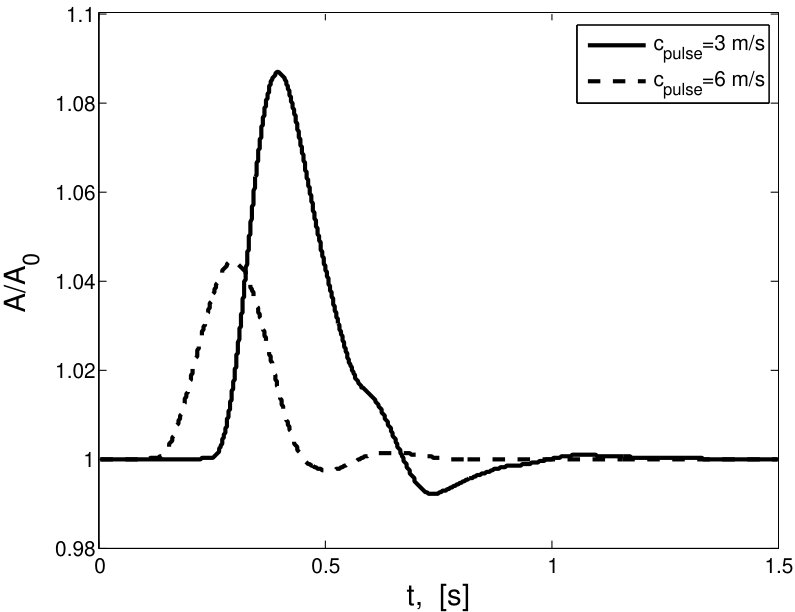 Figure 2
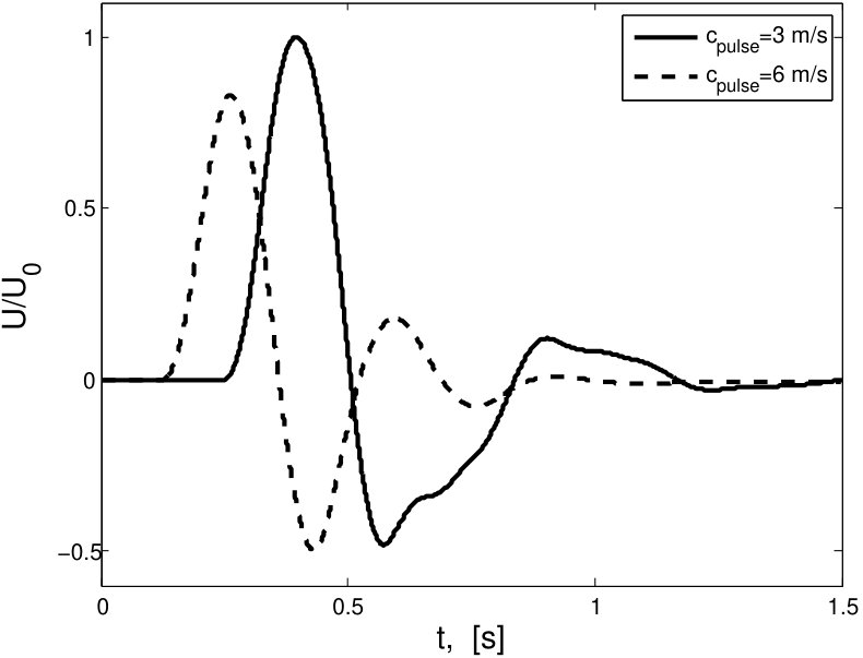 Figure 3
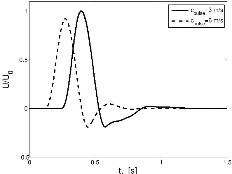 Figure 4
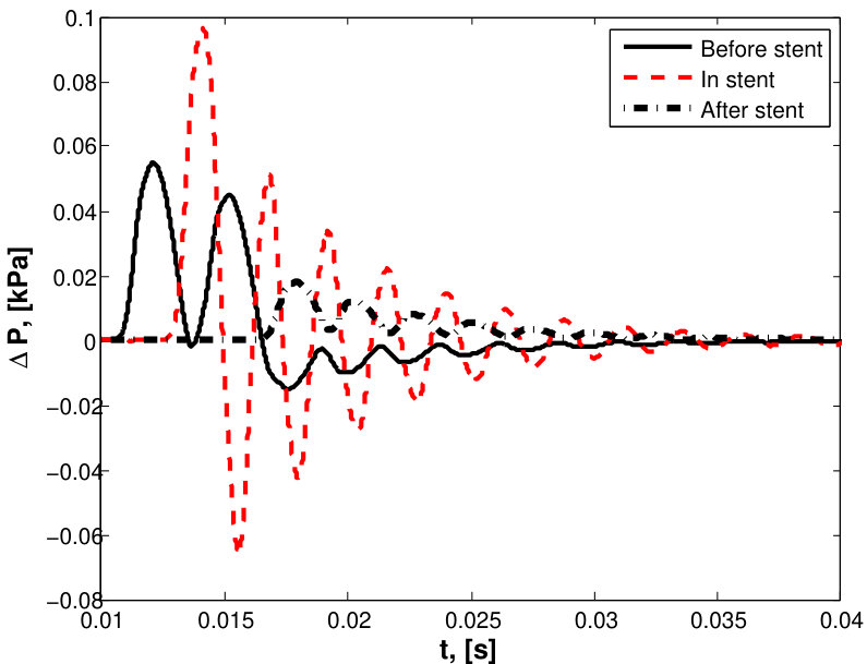 Figure 5
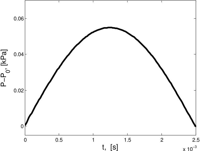 Figure 6
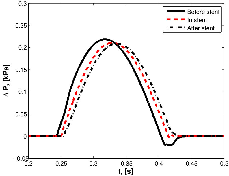 Figure 7
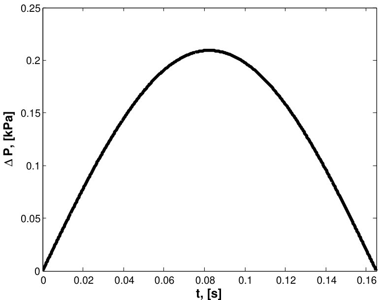 Figure 8
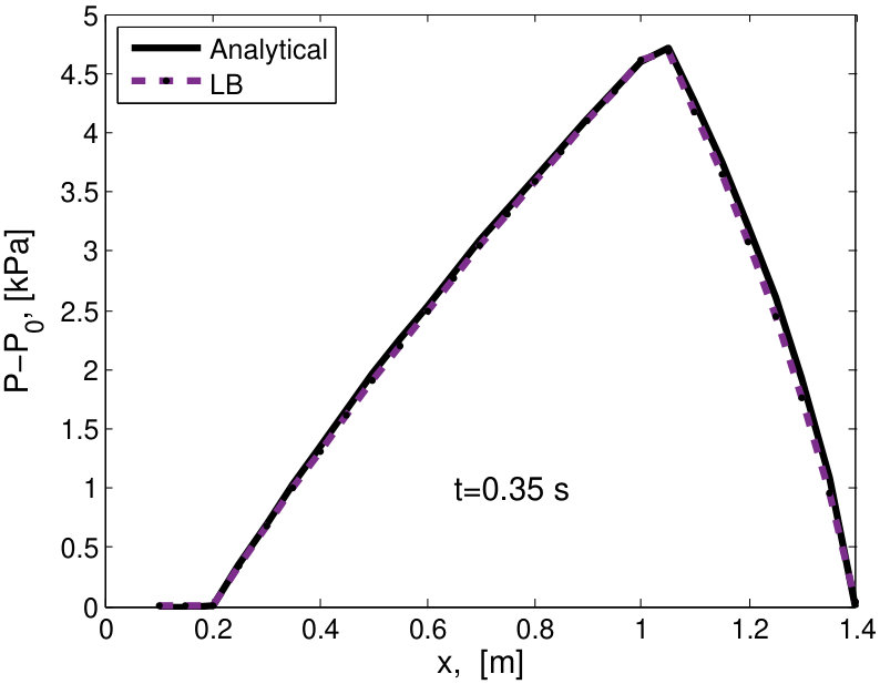 Figure 9
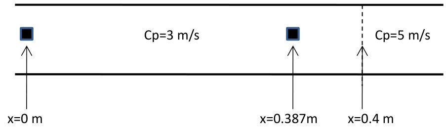 Figure 10
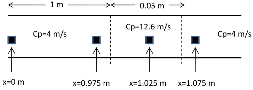 Figure 11
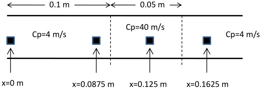 Figure 12
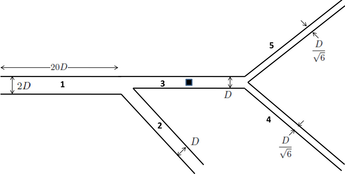 Figure 13
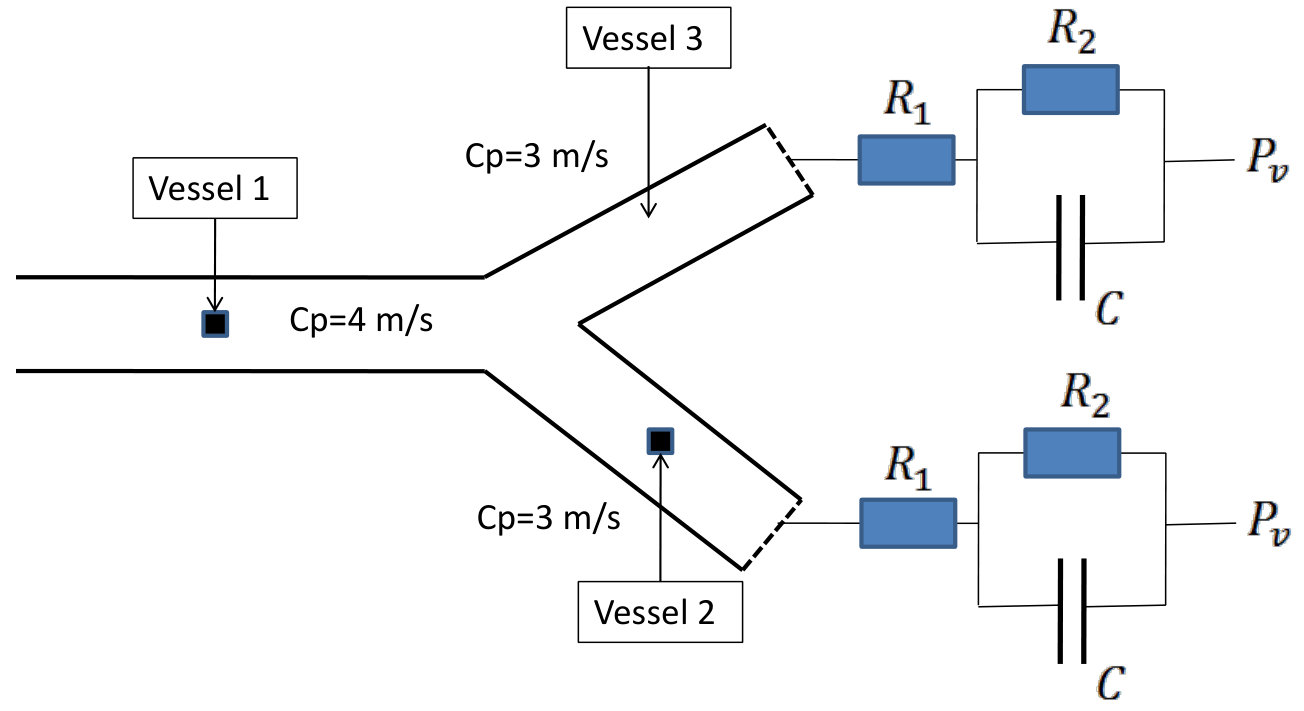 Figure 14
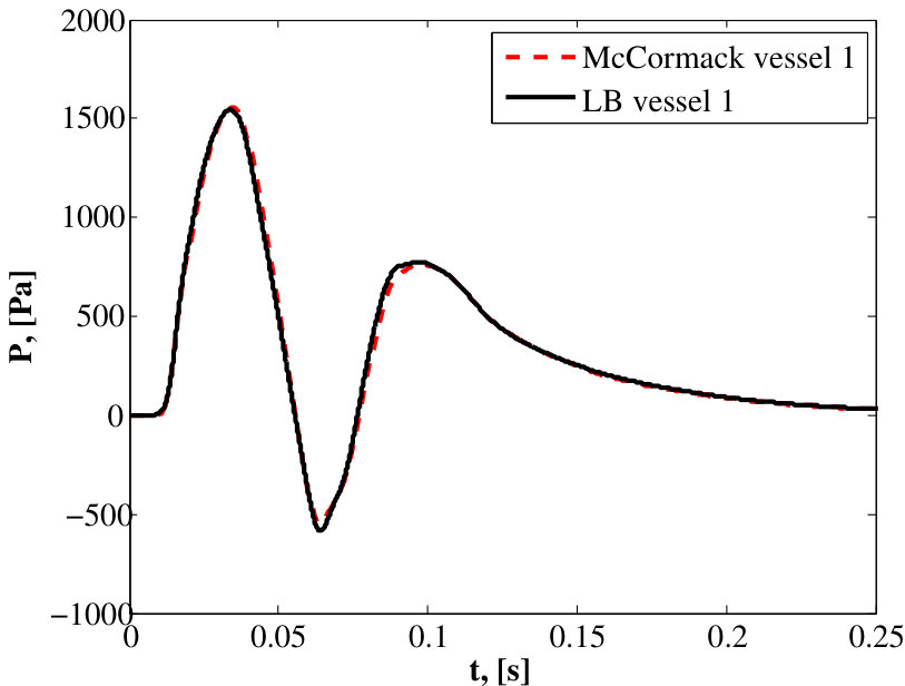 Figure 15
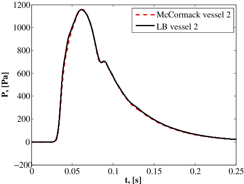 Figure 16
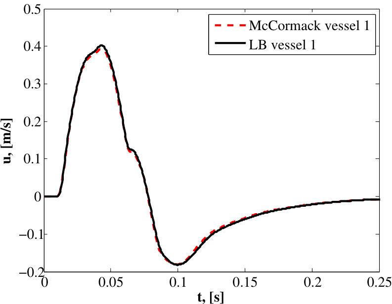 Figure 17
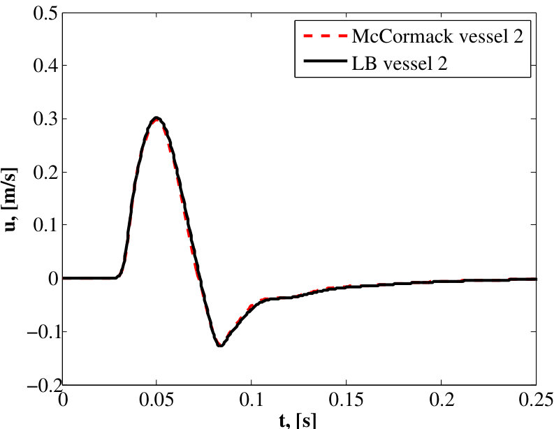 Figure 18
Peer Reviews
No public reviews on file for this paper yet. If you reviewed it on a platform where reviews are public (OpenReview, ICLR, NeurIPS, ICML), you can paste yours below so the community can read it here.
Videos
No videos yet. Explain this paper in a talk, walkthrough, or lecture? Add one.
The application of the Lattice Boltzmann method to the one-dimensional modeling of pulse waves in elastic vessels
Oleg Ilyin
Dorodnicyn Computing Centre of Russian Academy of Sciences, Vavilova st. 40, 119333 Moscow, Russia
Abstract
The one-dimensional nonlinear equations for the blood flow motion in distensible vessels are considered using the kinetic approach. It is shown that the Lattice Boltzmann (LB) model for non-ideal gas is asymptotically equivalent to the blood flow equations for compliant vessels at the limit of low Knudsen numbers. The equations of state for non-ideal gas are transformed to the pressure-luminal area response. This property allows to model arbitrary pressure-luminal area relations. Several test problems are considered: the propagation of a sole nonlinear wave in an elastic vessel, the propagation of a pulse wave in a vessel with varying mechanical properties (artery stiffening) and in an artery bifurcation, in the last problem Resistor-Capacitor-Resistor (RCR) boundary conditions are considered. The comparison with the previous results show a good precision.
keywords:
Lattice Boltzmann methods, Kinetic theory of gases and liquids, Biological fluid dynamics
1 Introduction
The models of blood motion in cardiovascular system vary from the [math]D lumped models, D pulse propagation equations to D viscous flow equations [1]. In many cases the D approach based on the solution of the Navier-Stokes equations is too detailed while [math]D lumped models are oversimplified and applicable only for the distal vasculature. In the case of the D models it is assumed that the radial velocity is negligible [2]. Then, integrating the Navier-Stokes equations over the radial variable the D nonlinear system of equations (depending only on one spatial variable, axial coordinate) for luminal area change (or pressure) and axial blood velocity is derived [3, 2]. Several numerical approaches for solving of these equations have been proposed including variations of Galerkin discretization [2, 4, 5], McCormack and Lax-Wendroff schemes [6, 7, 8, 9], trapezoidal schemes [10] and a relatively novel well-balance discretization method [11, 12]. The comparison results of the numerical methods can be found in [13, 14]. Among the open-source numerical solvers one can mention [math]D framework pyNS [15], D finite-volume OpenBF solver [16], Lax-Wendroff method based D solver VaMpy [17], finite element method based Artery.FE framework [18].
The hydrodynamic equations can be modeled using the kinetic methods like the Lattice Boltzmann approach [19, 20]. This method describes the motion of particles on a Cartesian spatial lattice (advection part), the collision of the particles is modeled by assuming that the velocity distribution of the particles tends to a local equilibrium state. The Lattice Bolzmann (LB) method correctly reproduces low-Mach incompressible flows like blood motion and can be used for the modeling of the flow in cardiovascular network.
The Lattice Boltzmann simulations of the blood flow dynamics in 2D and 3D vessel geometry have gained some popularity recently [21, 22, 23, 24, 25, 26]. The boundary conditions for LB models applied to blood flow problems in elastic tubes have been proposed in [21]. Several results are devoted to the estimation of blood endothelial (wall) shear stress in complicated vessel networks using LB approach, or using LB models coupled with Monte-Carlo simulations [22, 23, 24, 25, 27].
In the present paper an alternative way to model 1D blood motion equations based on the Lattice Boltzmann method is proposed. It is shown that there exists an analogy between the one-dimensional LB model D1Q3 with a virtual force (such approach is popular in modeling of non-ideal gas and multiphase flows using LB approach) at the limit of small Knudsen numbers (small times between collisions) and the blood flow equations in elastic vessels. More precisely, the LB hydrodynamics for D1Q3 model is equivalent to the 1D blood motion equations if one changes the sound velocity in the LB model by the pulse propagation velocity and the density by the vessel luminal area. The addition of the fictitious force allows to model arbitrary area-pressure vessel responses. The presented method is relatively simple in implementation.
Several test problems are considered. The method correctly describes the change in shape of the initial pulse wave while propagating along a vessel, the analytical solution profile is very close to the LB modeling results. The second test problem concerns the propagation of pulse waves with various amplitudes and duration in a vessel with a prosthesis [4, 28], in the next problem an artery network (5 vessels, 2 bifurcations) is considered [2]. Finally, the inclusion of the RCR boundary conditions for the LB model is discussed and LB simulation results are compared with McCormack difference scheme for the vessel branching supplemented with RCR boundary conditions at the distal ends of the daughter vessels.
2 Lattice Boltzmann approach for non-ideal gas and 1D blood flow equations in elastic vessels
2.1 The mass and momentum conservation equations for inviscid 1D blood flow in elastic vessels
Consider a long elastic vessel filled with incompressible fluid (blood). The conservation equations of mass and momentum in the elastic vessel are obtained from the Navier–Stokes equations by the integration over the cross-sectional spatial coordinate (radial variable). Assume that the radial component of the blood velocity is close to zero, and the velocity profile is flat. Then the following equations are obtained [2]
[TABLE]
where is the constant blood density (incompressible fluid), is the luminal area, blood velocity respectively and is the viscous drag force. Here is the axial coordinate and is the blood pressure.
It is obvious that one has three unknowns and only the two governing equations. To close the system (1) one needs to introduce a pressure-area relation
[TABLE]
where is a some function, its form should be defined from the elastic properties of the considered vessel. For realistic vessels this dependence can be complicated and saturation effects are observed [29]. In practice the Laplace law is popular [1, 2].
From the pressure-area relation one can find the pulse-wave velocity using the formula
[TABLE]
Using the pulse wave velocity definition Eqs (1)-(2) can be rewritten in the following equivalent form
[TABLE]
In the present paper the drag force is not considered, therefore .
2.2 The Lattice Boltzmann method and hydrodynamics
It will be sufficient to consider the simplest three-velocity model [19]. This model describes three populations of particles traveling on a 1D lattice with equal spacing between the lattice nodes. Here is the lattice velocity, is the lattice time step. During the discrete time step the particles at a node can hop to adjacent nodes or stay at the node . The concentrations of the particles traveling with the velocities are given by and respectively. The dynamics of obeys the following discrete equations in space and time
[TABLE]
[TABLE]
[TABLE]
where is the relaxation time which can be considered as a free parameter, are the components of an external force and are the equilibrium states (analogs of the Maxwell distribution)
[TABLE]
[TABLE]
[TABLE]
where are the lattice weights and are the density and flow velocity
[TABLE]
[TABLE]
moreover, one can define the full energy of the lattice gas in every node by the formula
[TABLE]
and here is the sound velocity of the lattice gas defined by
[TABLE]
Here the external force is taken in the linearized form [19]
[TABLE]
where is the force magnitude.
At the limit of small values of the lattice gas can be considered as continuous media since the time between collisions tends to zero ( is proportional to the expected time between particle collisions). In the continuous limit the considered LB model describes some hydrodynamics which can be obtained using the Chapman-Enskog expansion on a small parameter, the detailed analysis of this procedure for LB method in 1D case can be found in [30]. One has
[TABLE]
where is the spurious term which appears due to the quadratic form of the local equilibrium on the bulk velocity , is space-time discretization error ( LB scheme has second order accuracy) and is the gas viscosity. If the flow is slow (i.e the Mach number is small) and the time step is small then one can assert that the LB model correctly describes 1D hydrodynamics. It should be mentioned that the Navier-Stokes equations without spurious term can be obtained if high-order LB models are considered [31, 32]. In the present case the term proportional is unimportant since the blood flow is significantly subsonic.
2.3 The Lattice Boltzmann equation as a model of hemodynamics
One can see that the luminal area in the equations (4) is very similar to the density in the equations (5). If one changes the density by the luminal area and the sound velocity by the pulse wave velocity then Eqs (5) turn into Eqs (4) if the flow is slow, discretization error is negligible. These conditions are realistic due to a) for a typical blood flow the Mach number is over , [2] b) the discretization error can be controlled by the choice of .
The lattice Boltzmann approach gives slightly different longitudinal viscosity term than in Eqs (1)-(2) . This difference is unimportant since the terms are very close (same in the linear theory), moreover stream-wise diffusion effects play small role in hemodynamics and usually omitted from the consideration. In the present case the diffusion is an inherent property of the LB method.
One should emphasize that the force free case in the equations (5) describes only the particular case of constant pulse velocity since the sound velocity is constant, the blood flow equations are derived for the pressure-area relation in the form (this results from the definition of the pulse wave velocity (3)). The logarithmic dependence is only qualitatively correct, a more popular Laplace law states that , moreover the dependence of the pressure on the luminal area in real arteries is saturating [29], hence a generalization of the model is desirable.
The idea of the generalization of the presented approach is to choose the force term in such a way that the case of the non-constant pulse velocity is captured. This approach is similar to the method of modeling of non-ideal gases and phase transitions using LB schemes [33, 34, 35, 36, 37, 38]. Following the articles [35, 36, 38] the force is introduced using a pseudo-potential
[TABLE]
where is a some function. Using the expressions (6) the terms become in the hydrodynamic equations (5), next changing by and selecting in a such way that
[TABLE]
where is the desired pressure-area law one obtains the equations (4).
Following [36] the pseudo-potential can be written in the form , and for the LB model the central discretization of the spatial derivatives is adopted
[TABLE]
where is the lattice spatial step. For the LB D1Q3 model with the force discretization in the form (7) the stability conditions are known [36]
[TABLE]
From the relation (8) one can see that stability can be controlled by adjusting the lattice velocity .
The model implementation at the each time step consists of the two parts. Firstly, the collision term (right hand side of LB model) is computed in all spatial nodes and then the post-collision distribution functions are obtained. Next, the streaming step is performed .
2.4 Stability improvement
For the conventional LB method Courant-Friedrichs-Lewy (CFL) number (defined as ) equals to unity. This means that LB method is only marginally stable. This feature is well-known and several efforts have been paid to improve the stability properties, the possible solution is to rewrite the streaming step in such a form that LB model becomes a finite-difference scheme with controllable CFL number [39, 40, 41, 42, 43, 44].
The simplest way to decrease CFL number is the implementation of the fractional time step. In this method [40] the streaming part , where and is the post-collision distribution function is replaced by
[TABLE]
[TABLE]
where . For this realization of the streaming component the particles travel a distance during a time step and the parameter is Courant-Friedrichs-Lewy number. The form (9) guarantees second order accuracy in space and time. Finally, one should mention that for the LB model with the streaming step (9) the viscosity is governed by the relation [40].
In the present paper for the test problems in Paragraphs 3.1-3.3 the conventional streaming part () was applied, for the test problem in Paragraph 3.4 the fractional time step with was implemented.
3 The model application.
From the results of the previous paragraph one derives the following LB model
[TABLE]
[TABLE]
[TABLE]
[TABLE]
[TABLE]
where and , . The function is obtained from the equation
[TABLE]
here are the target pressure pulse velocity and pressure-area relation. The local equilibrium states are defined as
[TABLE]
where
[TABLE]
[TABLE]
The relaxation time should be taken small enough if the inviscid flow is modeled. Note that wall friction forces are not taken in account but potentially they can be implemented as an additional external force. The pulse pressure waves presented in figures are recovered with use of the pressure-area relation .
The case of LB model without external force corresponds to the following pressure-area relation
[TABLE]
For the hemodynamic modeling the following tube law is popular
[TABLE]
where are the vessel distensibility, blood pressure at rest, blood density and . The case corresponds to the Laplace law. The value of can be taken arbitrary since only is computed. It will be more convenient to use a linearized pressure pulse velocity instead of the distensibility
[TABLE]
3.1 A sole forward pulse wave propagation.
The evolution of the nonlinear wave which has triangle shaped form in the initial moment of time is considered in a semi-infinite vessel with constant elastic properties.
For a forward traveling wave one has the relation between the wave velocity and the luminal area [45]
[TABLE]
then the equations (1)-(2) reduce to a differential equation for
[TABLE]
The equation (16) is supplemented with the symmetric triangle-shaped initial-boundary condition at for , where is one heartbeat
[TABLE]
[TABLE]
[TABLE]
and
[TABLE]
The pressure-area relation (14),, which corresponds to the Laplace law is considered. The analytical solutions to this problem are obtained in [45]. For the sake of brevity this solution is not given here. The LB equations (10)-(12) are applied with the initial-boundary conditions (17)-(20) and the modeling results are compared with the analytical solutions at . The modeling constants are given in Fig. 1 caption. A very good agreement between the solutions is observed ( Fig. 1).
3.2 A pulse wave propagation in a vessel with prosthesis.
A semi-infinite vessel with an interior stiff region (stent or prosthesis) is considered. Similar test problem was investigated using Galerkin and Taylor-Galerkin finite difference methods in the papers [28, 4].
The mass flow and full energy are continuous across the junctions of the stiff and elastic regions [46, 2]. Then
[TABLE]
where and denote left and right side of the junction interface respectively and is the blood density. Since the blood flow is slow then and one can consider the pressure continuity property instead of the full energy. Consider the Laplace area-pressure relation (14), . Using the linearized pressure pulse wave velocity the Laplace law reads
[TABLE]
The continuity condition at the junction is considered for the pressure-area relation linearized near , i.e. . In a similar way one can linearize the logarithmic tube law (13).
In terms of LB variables the continuity of the mass flux and the linearized pressure take the following form
[TABLE]
[TABLE]
[TABLE]
where the junction is placed between the lattice nodes ; are the LB velocities on the left and right sides from the junction; are the LB spatial steps and is the LB time step; are the force magnitudes on the left and right sides of the junction interface; and are the linearized pulse wave velocities. For the present problem the lattice velocities are taken as . Such a calibration is convenient and guarantees that the lattice sound velocity equals to the linearized pulse wave velocity.
The distribution functions are unknowns, they are obtained from the continuity conditions
[TABLE]
[TABLE]
[TABLE]
[TABLE]
where
[TABLE]
For the test problems considered here it is assumed that the undisturbed vessel cross-sectional area equals , the blood density is .
The first vessel geometry is depicted in Fig. 2. The dynamics of a half-sinusoidal pressure pulse wave with the maximal amplitude of and the duration of starting at the point is studied. The pressure-area relation (13) is adopted.
The distensibility of the prosthesis is assumed to be times smaller then in the other part of the vessel, therefore the linearized pulse wave velocity is is larger in the stiffening than in the remaining part of the vessel ( and ), Fig. 2.
The simulation results show that the pressure maximal magnitude is amplified (in the comparison with the wave at ) near the left junction with a subsequent pressure drop below the undisturbed level (Fig. 3). This behavior is in a good agreement with the results from [28, 4]. The pressure increase over the initial pressure values happens due to the reflection of the wave entering the stiff region while the pressure drop is observed due to the second reflection of the wave leaving the stiff region.
The second considered vessel geometry is depicted in Fig. 4. A relatively short vessel segment (Fig. 4) and a small pulse wave amplitude are taken. Such a choice guarantees that the nonlinear effects do not distort initial wave shapes and shock waves do not appear. The distensiblity of the stiff region is smaller than the elastic parts of the vessel, this means that the pulse wave velocity in the stiff region is times larger than in the the elastic segments. The Laplace pressure-area relation is adopted.
The modeling results are presented in Fig. 5. Multiple reflections propagating from the junctions are clearly visible. The positive amplitudes correspond to the reflections occurred at the left junction while the waves with negative pressure amplitudes correspond to the reflections at the right junction. Again, the wave form behavior is very similar to the results from [28, 4].
3.3 Bifurcations of arteries
Consider a bifurcation of vessels: an undisturbed luminal area and linearized pulse wave velocity for a parent vessel are defined as and the same quantities for daughter vessels are defined as . At the junction point it is assumed that the continuity of the pressure and the conservation of the flow are satisfied [2]
[TABLE]
[TABLE]
where are the blood velocity and pressure alteration from the diastolic value in the vessels .
For simplicity, the pressure continuity condition is considered in the linearized form for the pressure-area relation (14), then one has In terms of the LB variables the equations (21)-(22) read as
[TABLE]
[TABLE]
where and
[TABLE]
where is the lattice step in -s vessel, moreover
[TABLE]
where is the amplitude of the external force in -s vessel (the definition of the external virtual force is given in (6)). The time step is constant in all vessels, while the lattice velocities can be different, here is the lattice spatial step. The lattice velocities are taken in a such way that
[TABLE]
the latter property guarantees that the pulse wave propagation speed will be different if are non-equal in the vessels.
At the junction point the value of is unknown for the parent vessel and the values of are unknown for the daughter vessels , they should be found from the equations (23)-(24). One has
[TABLE]
where are calculated from the linear system
[TABLE]
[TABLE]
here , and the following notations are introduced
[TABLE]
It is assumed that the wave is absorbed by the vessel boundaries (the vessels are well-matched with the distal vasculature). In order to absorb the incident wave the impedance boundary conditions should be stated [47].
The modeling artery geometry is depicted in Fig. 6. The input velocity wave is prescribed to the left inlet of the vessel and has the following form for . The linearized pulse wave velocities are taken same in all vessels: in the first case the value is used, in the second case this velocity equals . The case of the increased pulse velocity corresponds to the more stiff vessels which results to the smaller amplitudes of luminal area changes (Fig. 7-8). The Laplace pressure-area relation is adopted for the present problem. For the first (left) bifurcation the linear reflection coefficient [46] is
[TABLE]
and equals [math] for the forward wave traveling to the junction from the the vessel , on the other hand, for the backward wave traveling to this junction from the vessel or this coefficient equals . The linear reflection coefficient at the second (right) junction equals for the forward wave in the vessel . The backward waves at the distal ends of the vessels and do not exist since the outlets of these vessels absorb incident waves. Thus, the wave is partially ”trapped” in the vessel 3.
The wave dynamics and multiple wave reflections are measured at the middle of the vessel , see Fig. 7-8. In Fig. 8 the modeling results are presented for the geometry in Fig. 6 where the vessels 4 and 5 have increased radius (). This results in smaller reflection coefficient and therefore smaller amplitudes of the reflected waves in comparison with the profiles in Fig. 7.
The problem with the geometry in Fig. 6 was also considered in the paper [2]. The presented area and velocity profiles are very similar to the data from [2].
3.4 RCR boundary conditions
Resistor-Capacitor-Resistor (RCR) boundary conditions [48, 49, 50] are very popular in hemodynamical modeling. These boundary conditions are analogous to electric circuit with two resistances and one capacitor (Fig. 9). The first resistance accounts for the distal part of the truncated vessel and is usually selected in such a way that there are no wave reflection in a junction between a vessel and RCR model, while the second resistor accounts for the drag forces in the distal arterioles, the capacitor term is responsible for the compliance of the arterioles. One has for the pressures and velocities at the distal ends of the vessels 2,3 the following equation
[TABLE]
the first order discretization of this equation is following
[TABLE]
where and is the time step for the difference scheme. It is assumed that the values are known.
Any traveling wave in a vessel can be separated into the forward and backward components by the rule
[TABLE]
Using (27) one has
[TABLE]
[TABLE]
then
[TABLE]
Next, we mention that
[TABLE]
since can be considered as the forward traveling wave with the velocity , where is the distal point of the considered vessel. Therefore, we have expressed via known functions . Then
[TABLE]
[TABLE]
Now one expresses via the lattice Boltzmann variables
[TABLE]
[TABLE]
where is the amplitude of the external force, , where are the linearized pulse velocity and undisturbed luminal area, is approximated as . The values are unknowns at the distal end of the vessel, they are found from the equations
[TABLE]
[TABLE]
The relations (32)-(33) define RCR boundary conditions for the LB model. Finally one can see that the unknown values of LB distribution functions at the right end of the vessel (distal end) are defined by , they can be represented as a sum of the forward and backward components (30)-(31) which in turn depend on (the formulas (28), (29)).
As a test problem the propagation of a pulse wave in a vessel network consisting of three vessels (one parent vessel and two daughter vessels) and one bifurcation connected with RCR models at the distal outlets of the daughter vessels is considered. The parent vessel has the length , the luminal radius equals , the linearized pulse wave velocity equals . For the daughter vessels the values of the vessel length, luminal radius, linearized pulse wave velocity are taken as respectively. The Laplace law is adopted for the pressure-area relation. The initial pressure profile has the duration of and the maximal amplitude corresponding to luminal area increase in the vessel 1. The value of equals , where are the linearized pulse velocity and undisturbed luminal area respectively. The full resistance and compliance are taken as respectively, then the diastolic decay time .
The choice of the modeling parameters results in relatively complicated behavior of the pressure wave: since the linear reflection coefficient is negative for the vessel 1 at the branching point () the negative pressure wave component appears with subsequent positive backward wave caused by the microcirculation (Fig. 10, upper figure); the pressure component in the vessel 2 contains the forward pressure wave passed through the bifuracation and the backward pressure wave caused by the microcirculation (Fig. 10, lower figure).
As a benchmark solution the modeling results for the second order McCormack difference scheme [7] are adopted. For the McCormack scheme at the bifurcation point the continuity equations for the flux and pressure are considered jointly with the requirement that the characteristic variables are constant [2]. The realization of the boundary conditions at the vessel junction for the McCormack scheme differs from the LB approach (25)-(26) in which the characteristics are not considered.
The pressure and velocity profiles measured at the middle of the vessels are depicted in Fig.10 and Fig.11 for LB model and McCormack difference scheme. Both methods give very similar profiles, small differences are observed at some points, they can be attributed to the different approximation methods of the boundary conditions at the vessel bifurcations.
4 Conclusion
In the present paper the method for modeling of the 1D blood flow equations in elastic vessels using kinetic LB approach is proposed. The inclusion of the virtual external force in LB model allows to mimic arbitrary vessel luminal area response to the exerted blood pressure. Several test problems are considered.
In comparison to the conventional numerical methods of 1D blood flow modeling LB approach has the following distinctive features.
- In LB approach the viscosity of the fluid is the inherent property and its value is linearly dependent on . This property can be valuable for the modeling of lengthy vessel networks in which the diffusion effects are non-negligible.
- The implementation of the boundary conditions for junctions presented in the paper differs from the conventional realization. In the presented method the characteristics are not considered, the conditions for the pressure and the velocity in the junction are written explicitly in terms of LB variables. It is also possible to implement these boundary conditions in a standard way by expressing the characteristics in terms of LB variables (in a similar way like RCR conditions are introduced). The modeling results of LB approach are very similar (not exactly the same) to the pressure and velocity profiles obtained with use of the MacCormack scheme with the application of the conventional boundary conditions at the junctions.
- The abrupt changes in materials properties are allowed in the presented approach. Note that for some discrete methods the discontinuities in elastic properties are inadmissible [4]. On the other hand the inclusion of the vessel parts in which the pulse wave velocity changes smoothly over a some spatial region is not trivial for the presented method. 4. In LB approach the advection is linear (streaming part is linear) while for the conventional methods the discretization of the nonlinear terms should be considered. The linearity of the advection part is an attractive property for the parallel multi-CPU implementation of LB method.
The implementation of viscoelastic vessel response was not considered in the present paper. Potentially the viscoelastic effect can be inserted in the virtual force term. This term will contain an approximation of the vessel area time derivative (Kelvin-Voigt model), therefore an additional theoretical question about the stability of the scheme should be considered. This question is leaved for the future study.
The reference list from the paper itself. Each links out to its DOI / PubMed record.
- 1[1] C. Taylor, M. Draney, Experimental and computational methods in cardiovascular fluid mechanics, Rev. Fluid Mech. 36 (2004) 197–231.
- 2[2] S. Sherwin, V. Franke, J. Peiró, K. Parker, One-dimensional modelling of a vascular network in space-time variables, J. Engng. Math. 47 (2003) 217–250.
- 3[3] T. Hughes, J. Lubliner, On the one-dimensional theory of blood flow in the larger vessels, Math. Biosci. 18 (1973) 161–170.
- 4[4] L. Formaggia, D. Lamponi, A. Quarteroni, One-dimensional models for blood flow in arteries, J. Engng. Maths 47 (2003) 251–276.
- 5[5] J. Mynard, P. Nithiarasu, A 1d arterial blood flow model incorporating ventricular pressure, aortic valve and regional coronary flow using the locally conservative galerkin (lcg) method, Commun. in Numer. Meth. in Eng. 24 (2008) 367–417.
- 6[6] R. Mac Cormack, The effect of viscosity in hypervelocity impact cratering, J. Spacecraft Rockets 40 (2003) 757–763.
- 7[7] C. Hirsch, Numerical Computation of Internal and External Flows: The Fundamentals of Computational Fluid Dynamics, Butterworth-Heinemann, 2007.
- 8[8] M. Olufsen, C. Peskin, W. Kim, E. Pedersen, A. Nadim, J. Larsen, Numerical simulation and experimental validation of blood flow in arteries with structured-tree outflow conditions, Annals of Biomed. Engin. 28 (2000) 1281–1299.