Low-pass filtering as Bayesian inference
Cristobal Valenzuela, Felipe Tobar

TL;DR
This paper introduces a Bayesian nonparametric approach for low-pass filtering of time series that effectively manages uneven sampling and noise, using Gaussian process latent factors for precise inference.
Contribution
It presents a novel Bayesian nonparametric model for low-pass filtering that allows exact training and handles irregularly sampled, noisy data efficiently.
Findings
Outperforms standard linear filters on synthetic data
Effective on real-world time series with uneven sampling
Allows exact Bayesian inference with minimal approximations
Abstract
We propose a Bayesian nonparametric method for low-pass filtering that can naturally handle unevenly-sampled and noise-corrupted observations. The proposed model is constructed as a latent-factor model for time series, where the latent factors are Gaussian processes with non-overlapping spectra. With this construction, the low-pass version of the time series can be identified as the low-frequency latent component, and therefore it can be found by means of Bayesian inference. We show that the model admits exact training and can be implemented with minimal numerical approximations. Finally, the proposed model is validated against standard linear filters on synthetic and real-world time series.
Click any figure to enlarge with its caption.
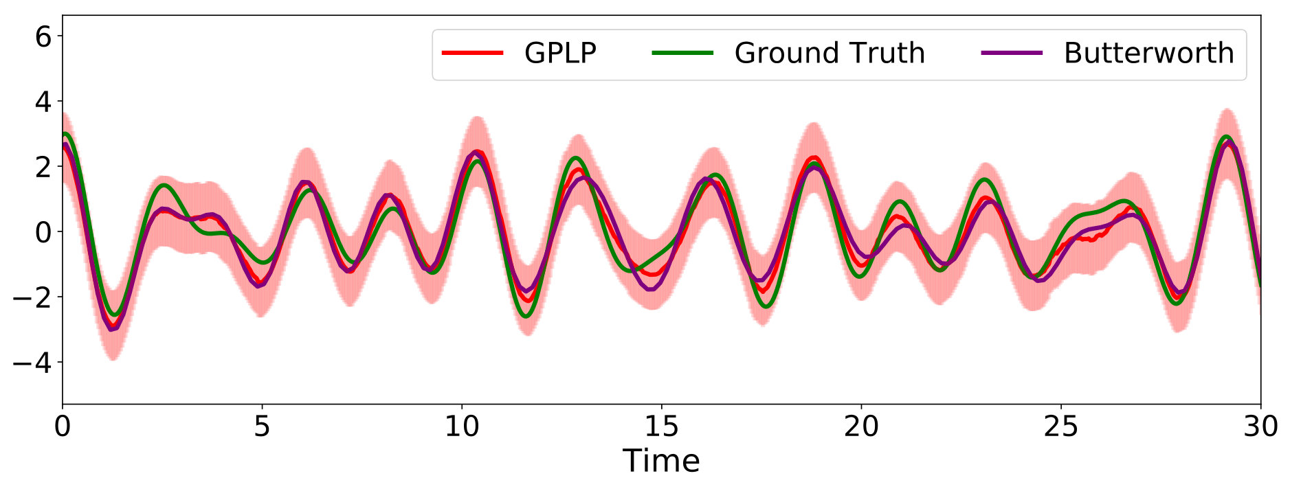 Figure 1
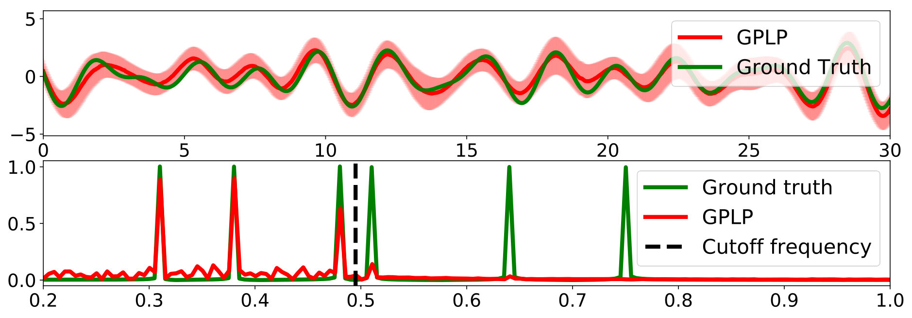 Figure 2
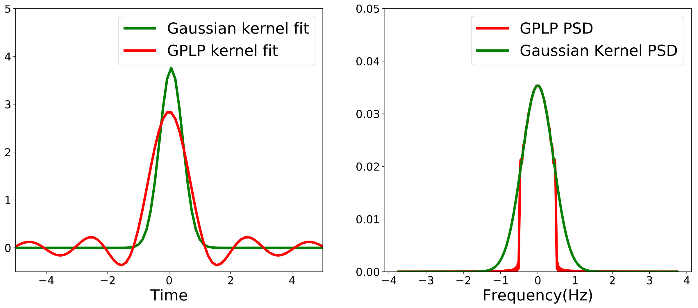 Figure 3
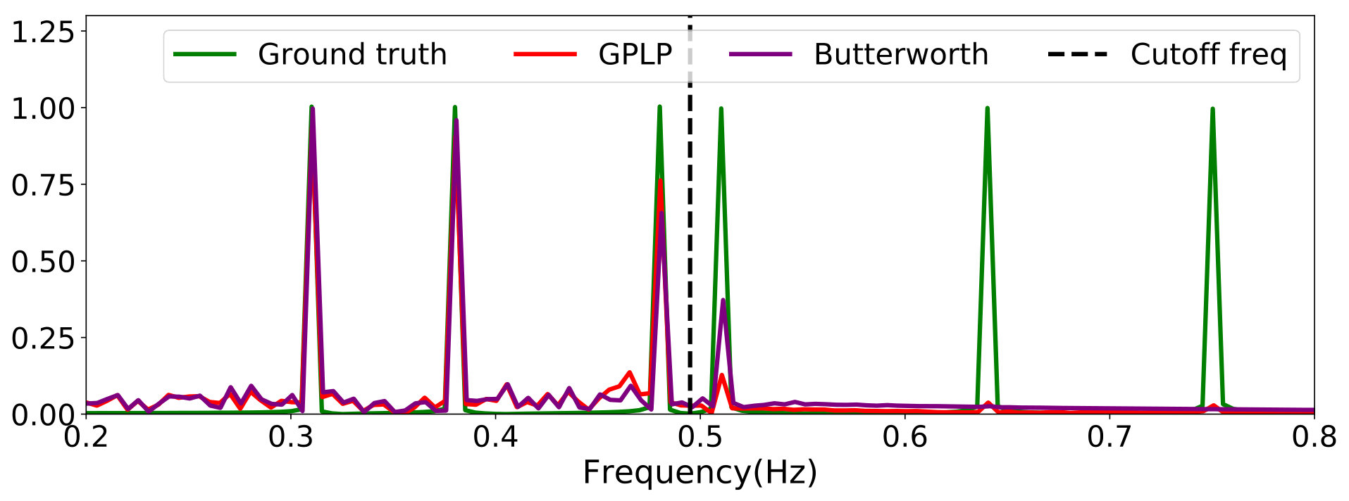 Figure 4
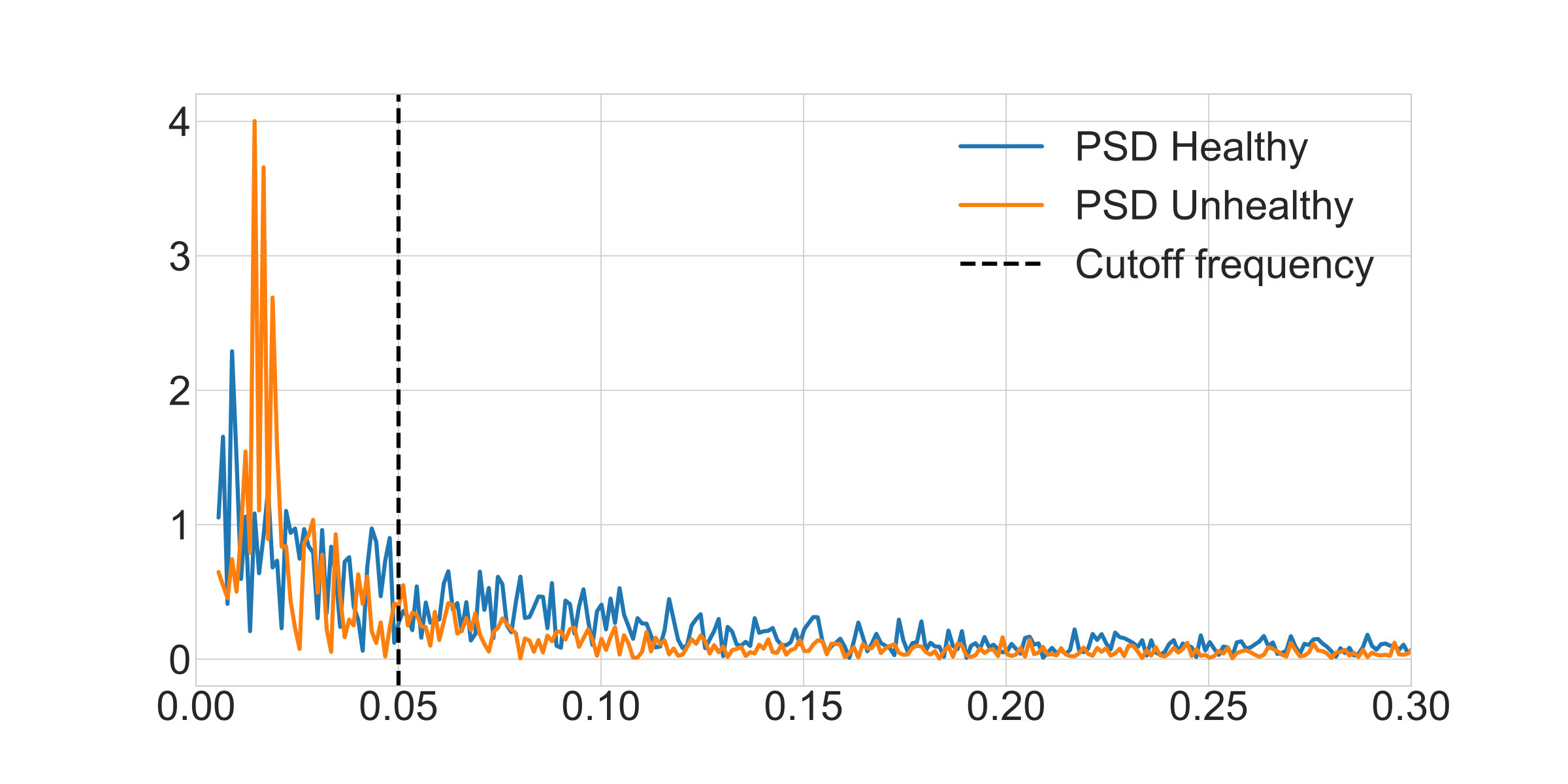 Figure 5
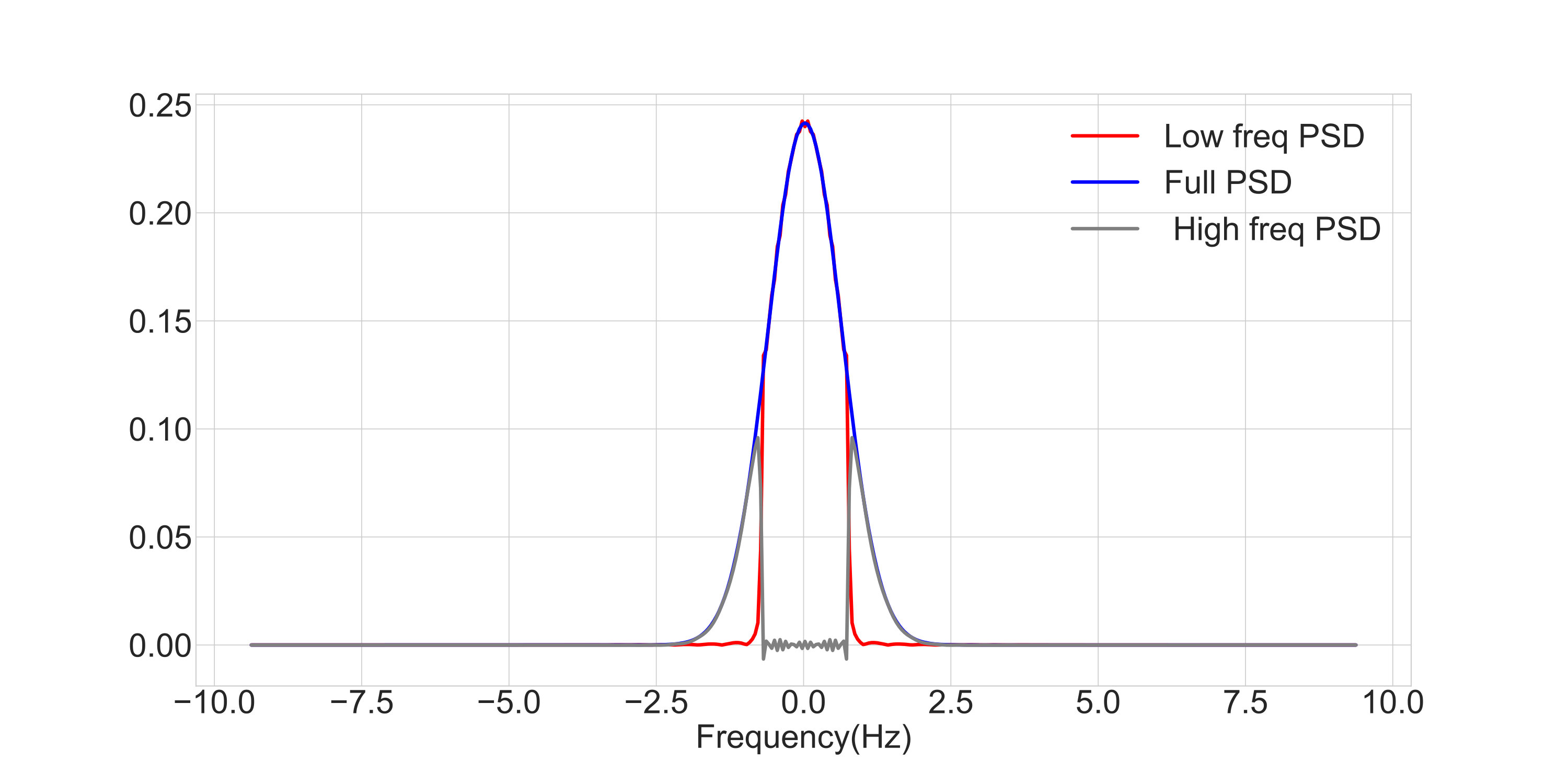 Figure 6
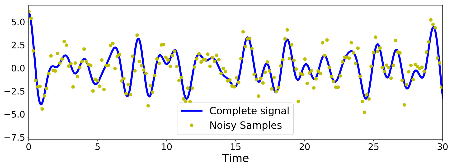 Figure 7
Peer Reviews
No public reviews on file for this paper yet. If you reviewed it on a platform where reviews are public (OpenReview, ICLR, NeurIPS, ICML), you can paste yours below so the community can read it here.
Videos
No videos yet. Explain this paper in a talk, walkthrough, or lecture? Add one.
Taxonomy
TopicsGaussian Processes and Bayesian Inference · Time Series Analysis and Forecasting · Target Tracking and Data Fusion in Sensor Networks
Low-pass filtering as Bayesian inference
Abstract
We propose a Bayesian nonparametric method for low-pass filtering that can naturally handle unevenly-sampled and noise-corrupted observations. The proposed model is constructed as a latent-factor model for time series, where the latent factors are Gaussian processes with non-overlapping spectra. With this construction, the low-pass version of the time series can be identified as the low-frequency latent component, and therefore it can be found by means of Bayesian inference. We show that the model admits exact training and can be implemented with minimal numerical approximations. Finally, the proposed model is validated against standard linear filters on synthetic and real-world time series.
Index Terms— Spectral estimation, nonunformly-sampled data, Gaussian process, low-pass filters, Bayesian inference.
1 Introduction
Monitoring the spectral content of a time series is of critical importance in real-world applications across a wide range of scientific disciplines. This is because the concentration of energy at a specific range of frequencies might be indicative of mechanical faults [1], cardiac anomalies [2], astronomical discoveries [3, 4], and whale calls from submarine audio recordings [5] to name a few.
The standard practice to isolate components within a specific frequency range from a time-series observation, referred to as filtering, is to convolve the observations with an object called linear filter. This convolution removes all frequencies that do not correspond to the desired frequency range, thus, filtering out unimportant frequencies. The theoretical rationale behind this approach is supported by the application of the Convolution Theorem [6] to power spectral densities (PSD): the PSD of a filtered time series corresponds to the PSD of the linear filter (user-designed) multiplied by the PSD of the observed time series (not controllable). This result allows for designing the linear filter so as to remove unwanted frequency components to then perform the numerical convolution. We refer to low-pass filtering when the range of frequencies to be removed are centred (symmetrically) around zero.
We identify two drawbacks of this standard approach to filtering. First, to perform the numerical convolution, the time series has to be uniformly sampled, that is, no missing observations or random acquisition times can be allowed. This is a rather stringent assumption, since in real-world applications missing data is commonplace due to mechanical or electrical failures and the sampling rate is given by the hardware. For instance, the observations of light curves in Astronomy are only available at some time instants due to climate conditions, orientation of the telescope and even the priority of the experiment within the agenda of the observatory. The second drawback of the convolution method is its implicit deterministic assumption: by computing a low-pass version of the time series as a moving average, we are accumulating observation noise without properly accounting for the dispersion that this might cause.
We aim to address these two drawbacks by formulating the low-pass filtering problem as a Bayesian inference one. We model the observed time series as a mixture of three latent components: one of low frequencies, one of high frequencies, and an observation noise component. Then, we find the low-frequency component through probabilistic inference: we place a prior distribution on each component and then, using observations of the time series, we find the posterior distribution over the low-frequency component. In particular, we choose Gaussian processes [7] priors over the components to leverage the expressiveness of the GP formulation while introducing minimal numerical approximations, therefore, the proposed method will be referred to as Gaussian process low-pass filter (GPLP).
2 Background: Gaussian Processes
2.1 Spectral representation of Gaussian processes
A Gaussian process (GP) [7] over the input set is a real-valued stochastic process , such that for any finite subset of inputs , the random variables are jointly Gaussian. Without loss of generality we choose . In this sense, a GP defines a distribution over real-valued functions , that is uniquely determined by its mean function , typically assumed to be zero, and its covariance kernel .
The covariance kernel summarises the dynamic behaviour of the GP and thus it is key when designing GP models. In practice, we can rely upon the Wiener-Khinchin theorem [8], which states that an integrable function is the covariance function of a weakly-stationary mean-square-continuous stochastic process if and only if it admits the representation
[TABLE]
where is a non-negative bounded function on and denotes the imaginary unit. Henceforth, given a kernel , we will refer to as their power spectral density given by the above theorem; where the PSD is the Fourier transform of the covariance kernel . This result allows us to encode spectral properties directly in the covariance function by first designing the PSD to then calculate the kernel as the inverse Fourier transform of the so designed PSD function.
The relationship between GPs and spectral representations has acquired attention recently in the machine learning community. For instance, covariance functions can be constructed in the spectral domain in parametric [9, 10] and nonparametric [11, 12] ways. Additionally, the harmonic structure of GPs has been exploited to develop computationally-efficient sparse GP models by using inducing variables in the spectral domain [13, 14, 15]. More recently, GPs have also been considered to address the spectral estimation problem, in particular, for nonuniformly-sampled data and detection of periodicities [16, 17, 18]. An open challenge in the spectral treatment of GPs, is that learning frequency representations is prone to local optima, since one aims to approximate a periodogram; this has been partially addressed using Bayesian optimisation with derivatives [19] and derivative-free Monte Carlo methods [20]. In our case, however, training simply involves a standard square exponential kernel (presented next) and therefore optimisation is straightforward.
2.2 The square exponential case
The de facto covariance kernel for GP models is the square-exponential covariance denoted by
[TABLE]
where the parameter denotes the marginal variance of the process (i.e., the magnitude) and denotes the lengthscale, that is, the range of correlation between values of the process: the larger the lengthscale the longer the range of temporal correlations.
The popularity of the SE kernel stems form its properties [7]. The paths generated by a GP with an SE kernel are (i) dense in the space of continuous functions, (ii) infinite-times differentiable a.e. and (iii) smooth, meaning that their power spectral density is concentrated around zero. In fact, due to the exponential form of the Fourier operator, the PSD of the SE kernel is also SE and given by
[TABLE]
where the lengthscale of this PSD (spectral domain) is now inversely proportional to the lengthscale of the covariance (temporal domain); this has key advantages when using GPs for spectral estimation [18, 14]. This can be understood intuitively: a process with long-range correlations has low frequency energy (smooth), whereas a kernel with short-length correlations necessarily has high frequency components (rough).
The generative model proposed in the next section will represent observed signals as a GP with SE covariance function composed of a mixture of (non overlapping) low- and high-frequency components.
3 A latent-component generative model for Bayesian filtering
We propose the following generative model for a continuous-time (latent) signal as a mixture of two components of the form
[TABLE]
where is a signal of low-frequency content and one of high-frequency content.
3.1 Assumptions over the spectral components and
We model and as independent GPs with covariance kernels denoted respectively by and , and, accordingly, power spectral densities and . To discriminate between higher and lower frequencies, we impose the following restrictions over and :
The support of , denoted by , is compact and centred around the origin, meaning that is a process of low-frequency content. 2. 2.
The supports of the PSDs of and are non overlapping, that is, . This implies that each frequency present in the signal came, exclusively, from either or . 3. 3.
The sum of the component PSDs is a square-exponential kernel, that is, for some hyperparameters and as in eq. (2).
Notice that, as a consequence of the third restriction, the marginal distribution over the process is a Gaussian process with an SE kernel due to the linearity of the Fourier transform and the independence of and .
Figure 1 illustrates the PSDs of the components of high and low frequency. We have denoted by the interface between the zones of low and high frequency, meaning that is the highest frequency of the low-frequency signal and well as the lowest frequency of the high-frequency signal. Consequently, the bandwidth of the low-frequency part is .
3.2 Likelihood and model fitting
Assuming an independent sequence of Gaussian observation noise, the observations are then defined as
[TABLE]
Combining the observation model defined in eq. (5) with the GP-prior assumed for the spectral components, the marginal likelihood of the proposed model is Gaussian and therefore its hyperparameters can be obtained through minimisation of the negative log-likelihood (NLL). Notice that despite the elaborate frequency-wise construction of the latent process through the non-overlapping spectra of the components and , the covariance kernel of is square-exponential, thus allowing for straightforward model learning. Specifically, the NLL of the model is given by
[TABLE]
where are the (noise corrupted and possibly missing) observations acquired at time instants , and is the covariance matrix of defined by
[TABLE]
therefore, the hyperparameters are those of the kernel and the noise variance .
Finally, observe that the strict non-overlapping property of the components and is not problematic for training, in fact, the cutoff frequency does not even appear for model training.
4 Filtering as posterior inference
Denote by the required cut-off frequency of the low-pass filtering problem. Using the proposed model, we can assume that this cutoff frequency is equal to the limit between the low- and high-frequency components. In this context, low-pass filtering problem is equivalent to performing inference over the low-frequency component conditional to observations of the time series. Due to the assumptions made on the signal we refer to this approach as GP low-pass filter (GPLP).
Denoting the observations by , GPLP addresses low-pass filtering by computing the posterior distribution . Due to the self-conjugacy of the Gaussian distribution and its closure under additivity, this posterior is also a GP, with mean and covariance given by
[TABLE]
where we have assumed zero mean for and (and therefore of ), is the covariance of the observations defined in eq. (7), denotes the covariance between and , and is the kernel of .
Let us also note that the cross covariance and the kernel share the same expression. Denoting the covariance between the low-frequency process at time and the observation at time by , we obtain
[TABLE]
since the processes , and are independent Gaussian processes.
Therefore, the only critical quantity required to compute eqs. (8)-(9) is kernel . Following the model proposed in eq. (4) and its assumptions, the PSD of , denoted by , can be obtained by multiplying the PSD of with a rectangular function of width , that is,
[TABLE]
where we used the convention that is equal to one for and 0 elsewhere. As a consequence, the kernel can be calculated using the convolution theorem: ( is the convolution operator)
[TABLE]
where denotes the error function given by
[TABLE]
Using Taylor expansions, the error function can be calculated up to an arbitrary degree of accuracy [21].
5 Simulations
The proposed model for Bayesian low-pass filtering using GPs, termed GPLP, is next validated using synthetic and real-world data. Our experimental validation aims to show that GPLP (i) successfully recovers low-frequency data from missing and noisy observation, (ii) provides accurate point-estimates with respect to the benchmarks, and (iii) places meaningful error bars. Our benchmarks include ground-truth signals and the Butterworth filter.
5.1 A synthetic time series with line spectra
We considered the line-spectra time series given by
[TABLE]
were the sets and are such that . Simply put, is a set of low frequencies and a set of high frequencies—all these frequencies are in Hertz (Hz). Signals constructed in this way have sparse PSDs meaning that only a finite number of frequencies convey all the signal energy or information.
We chose and and simulated a path of , as defined in eq. (13) for 5000 evenly-spaced time indices in . The observation time-series consisted only in a 25% of the signal (again, evenly spaced) all of which were corrupted by Gaussian noise of std. dev. . Fig. 2 shows the latent signal and the observation considered for this experiment.
We implemented the proposed GPLP to recover the low-frequency content of the original (latent) signal only using the observations . We first trained the generative model as explained in Sec. 3.2 to find the hyper parameters , and . We then chose the cutoff frequency to be Hz. We then computed the low-frequency covariance function to calculate the moments of the posterior distribution . Fig. 3 shows the learnt kernels and their corresponding PSDs. Notice how, just as illustrated in Fig. 1, the spectral densities of the latent low-frequency component is band-limited, supported only on and tightly bounded by the (unfiltered) time series.
Fig. 4 shows the GPLP estimate compared against the ground truth and a low-pass version of the data using a Butterworth low-pass filter of order , with the same cutoff frequency; this filter is a standard in linear filtering. GPLP obtained a mean-squared error of while the Butterworth low-pass filter gave a mean-squared error of , in addition to this marginal difference in performance, notice that GPLP provided accurate 95% error bars.
To further validate the ability of the proposed GPLP to filter out low-frequency spectral content, Fig. 5 shows the Fast Fourier Transform (FFT) of the low-pass versions of GPLP, Buttwerworth and the original signal. Notice from that GPLP successfully recovered the first three spectral components and rejected the higher ones.
5.2 Low-pass filtering of unevenly-sampled observations
A critical downside of the standard filtering techniques is that most of them require the data to be evenly spaced. Here is where the proposed model excels: as our method is based on an infinite-dimensional prior over continuous-time signals, missing observations are naturally handled by integrating out missing values.
We replicated the exact same setting as in Sec. 5.1 but considered randomly-chosen observations (Again, just of the total number of points). Fig. 6 shows the posterior mean over the low-frequency component together with the 95% confidence interval and the ground truth, as well as the result in the frequency domain. The MSE of the GPLP estimate was , thus improving over Butterworth using evenly spaced data.
5.3 Filtering a heart-rate time series
We considered two 1800-sample heart-rate signals111http://ecg.mit.edu/time-series/. One corresponding to a healthy subject and an unhealthy subject. The anomally can be detected from the heart-rate signal by looking at the energy contained below (Hz): if most of the energy is below this threshold, the subject is likely to suffer from congestive heart failure [22].
The aim of this experiment was to use GPLP to quantify the portion of energy below , as this reveals whether the signal corresponds to a healthy or unhealthy subject. We implemented GPLP on both signals with a cutoff frequency of and we found that the healthy signal has a 77% of its energy below and that the unhealthy signal has a 97% of its energy below . Therefore, the GPLP method can discriminate between healthy and unhealthy subjects from the heart-rate signals.
6 Discussion
We have proposed a Bayesian approach to low-pass filtering. The method is based on a latent-component generative model for time series, where the components are Gaussian processes with non-overlapping spectra. With this model, finding the low-pass version of a signal can be addressed from a Bayesian inference point of view. The main contribution over existing low-pass filters in the linear filter literature is that the proposed model offers an account of its own uncertainty and can naturally handle missing or noisy observations.
The proposed method has been validated empirically using synthetic and real-world data, where we have shown its ability to recover unbiased estimates of the true low-frequency signals (both in the evenly- and unevenly-sampled cases) and performed accurately with respect to its classical counterpart: the Butterworth filter.
7 Acknowledgements
This work was funded by projects Fondecyt-Iniciación #11171165 and Conicyt-PIA #AFB170001 Center for Mathematical Modeling.
The reference list from the paper itself. Each links out to its DOI / PubMed record.
- 1[1] D.-H. Kwak, D.-H. Lee, J.-H. Ahn, and B.-H. Koh, “Fault detection of roller-bearings using signal processing and optimization algorithms,” Sensors (Basel, Switzerland) , vol. 14, pp. 283–298, 12 2013.
- 2[2] F. Tobar, G. Rios, T. Valdivia, and P. Guerrero, “Recovering latent signals from a mixture of measurements using a Gaussian process prior,” IEEE Signal Processing Letters , vol. 24, pp. 231–235, 2017.
- 3[3] S. E. Whitcomb and J. Keene, “Low-pass interference filters for submillimeter astronomy,” Appl. Opt. , vol. 19, no. 2, pp. 197–198, Jan 1980.
- 4[4] L. Araya-Hernández, J. F. Silva, A. Osses, and F. Tobar, “A Bayesian mixture-of-Gaussians model for astronomical observations in interferometry,” in Proc. of Chilecon , 2017, pp. 1–5.
- 5[5] A. Cuevas, A. Veragua, S. Español-Jiménez, G. Chiang, and F. Tobar, “Unsupervised blue whale call detection using multiple time-frequency features,” in Proc. of Chilecon , 2017, pp. 1–6.
- 6[6] Y. Katznelson, An Introduction to Harmonic Analysis , Cambridge Mathematical Library. Cambridge University Press, 3 edition, 2004.
- 7[7] C. E. Rasmussen and C. K. I. Williams, Gaussian Processes for Machine Learning (Adaptive Computation and Machine Learning) , The MIT Press, 2005.
- 8[8] A. M. Yaglom, Correlation Theory of Stationary and Related Random Functions , Cambridge Mathematical Library. Springer-Verlag New York, 1 edition, 1987.