Lossless Source Coding in the Point-to-Point, Multiple Access, and Random Access Scenarios
Shuqing Chen, Michelle Effros, Victoria Kostina

TL;DR
This paper develops a unified analysis of lossless source coding in various scenarios, providing third-order performance characterizations and introducing a novel random access coding scheme with rateless coding and feedback.
Contribution
It introduces a third-order analysis for multiple scenarios and proposes a new random access source coding method with provable optimality.
Findings
Third-order characterization of Slepian-Wolf rate region.
Independent encoders can match joint encoder performance.
A rateless coding scheme with feedback achieves optimal performance.
Abstract
This work studies point-to-point, multiple access, and random access lossless source coding in the finite-blocklength regime. In each scenario, a random coding technique is developed and used to analyze third-order coding performance. Asymptotic results include a third-order characterization of the Slepian-Wolf rate region with an improved converse that relies on a connection to composite hypothesis testing. For dependent sources, the result implies that the independent encoders used by Slepian-Wolf codes can achieve the same third-order-optimal performance as a single joint encoder. The concept of random access source coding is introduced to generalize multiple access (Slepian-Wolf) source coding to the case where encoders decide independently whether or not to participate and the set of participating encoders is unknown {\em a priori} to both the encoders and the decoder. The proposed…
Click any figure to enlarge with its caption.
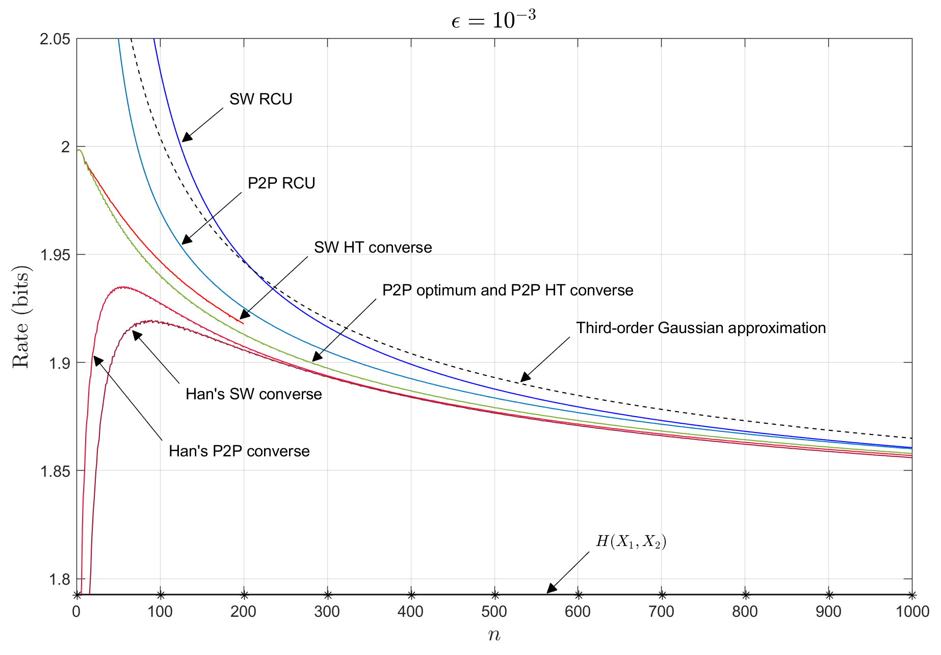 Figure 1
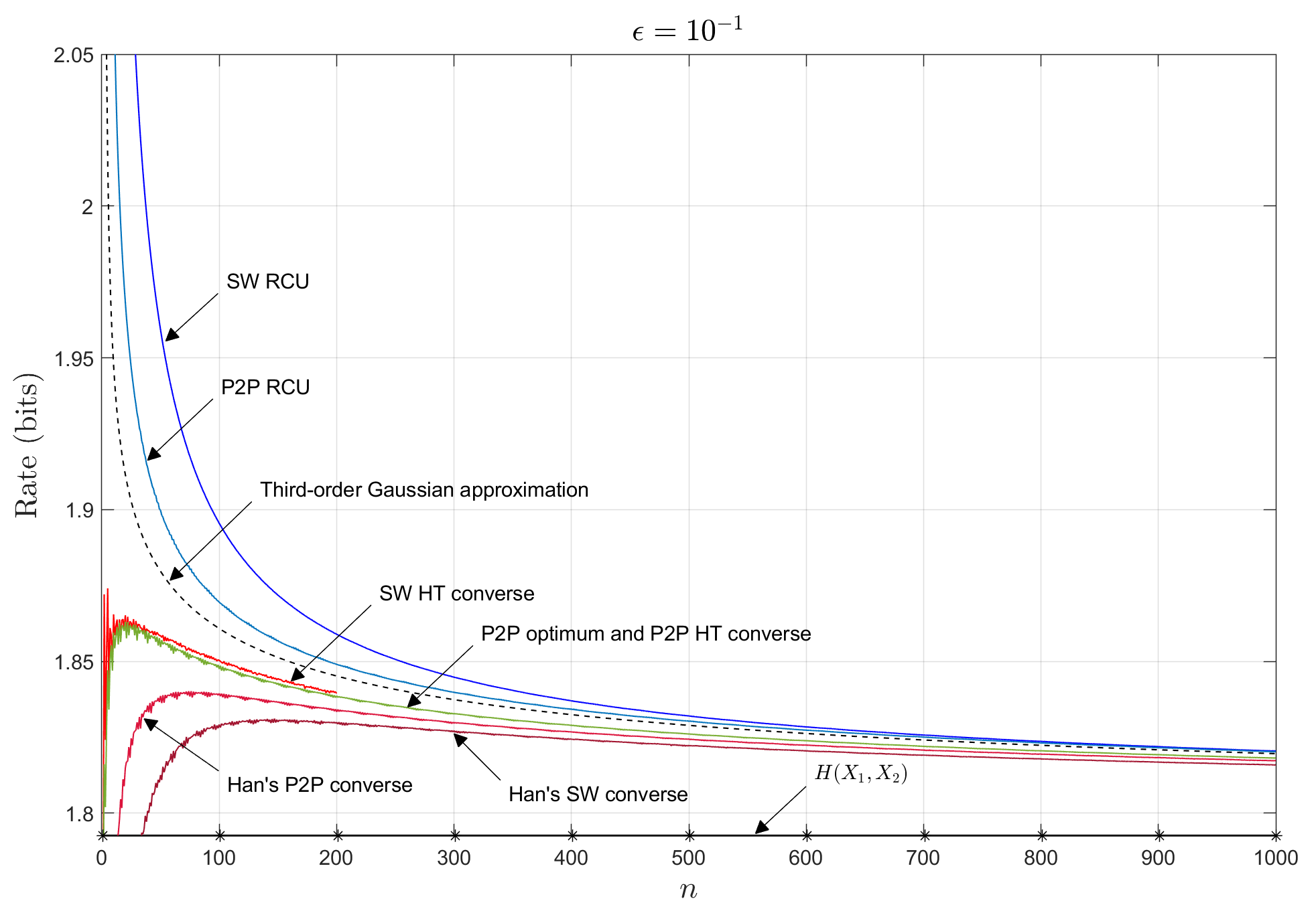 Figure 2
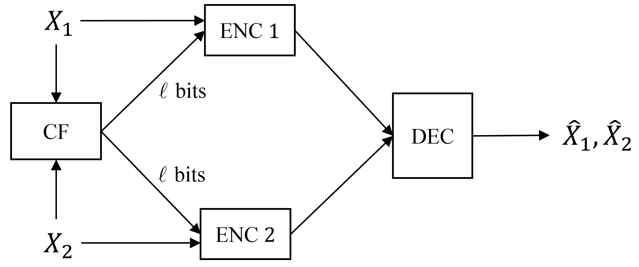 Figure 3
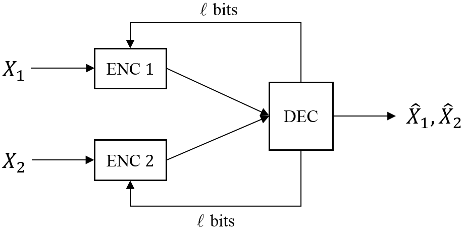 Figure 4
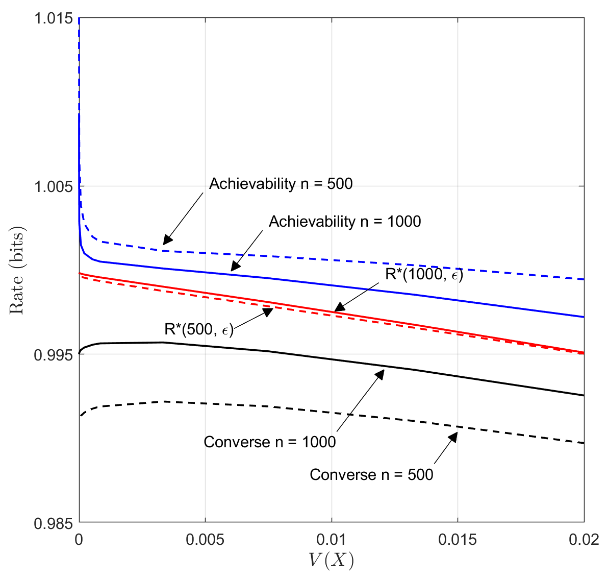 Figure 5
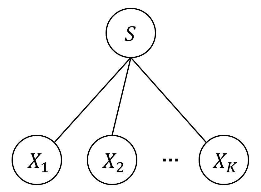 Figure 6
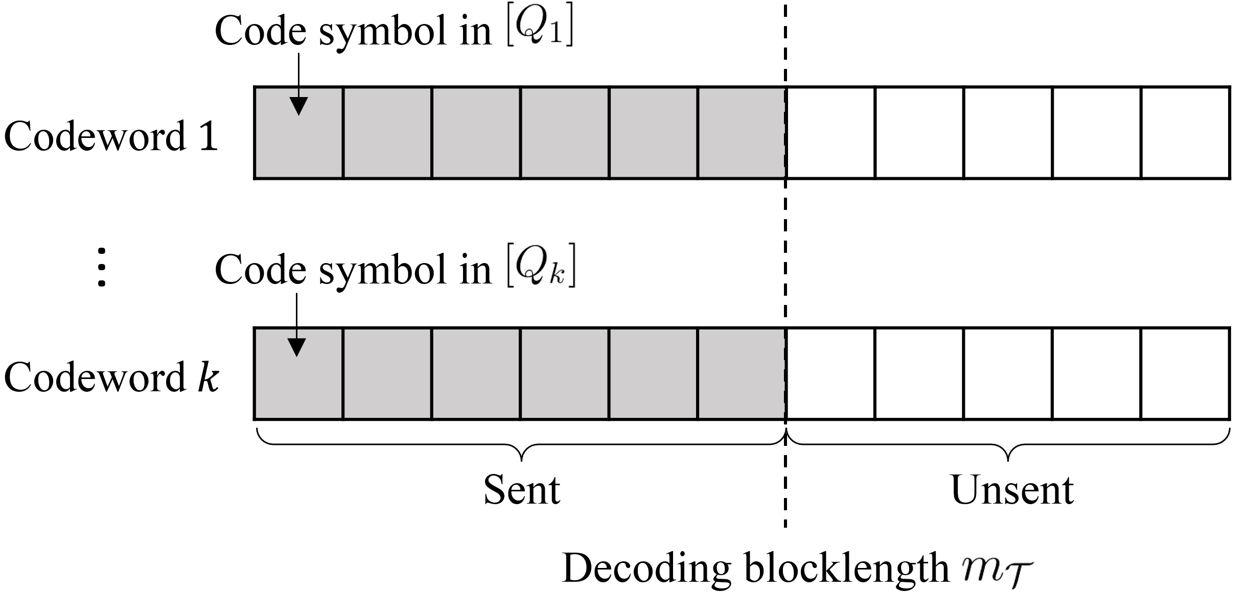 Figure 7
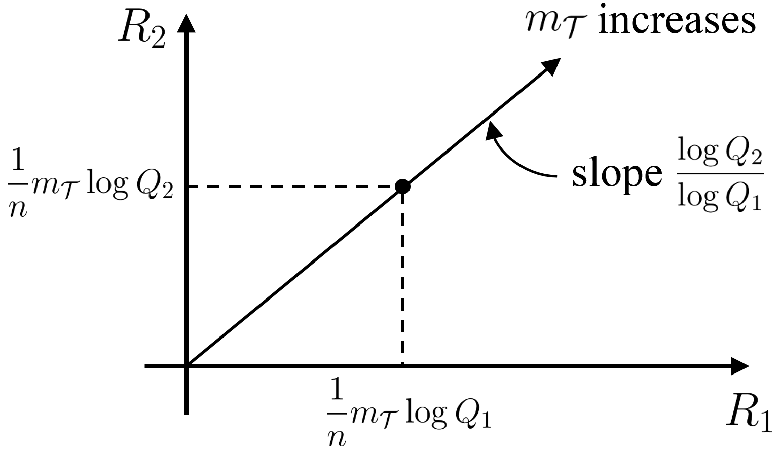 Figure 8
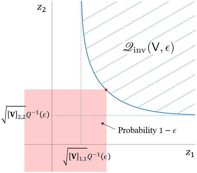 Figure 9
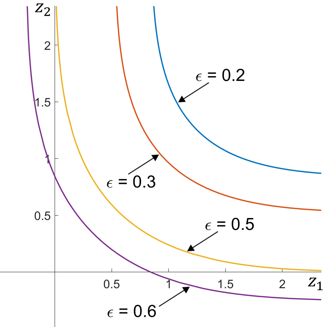 Figure 10
 Figure 11
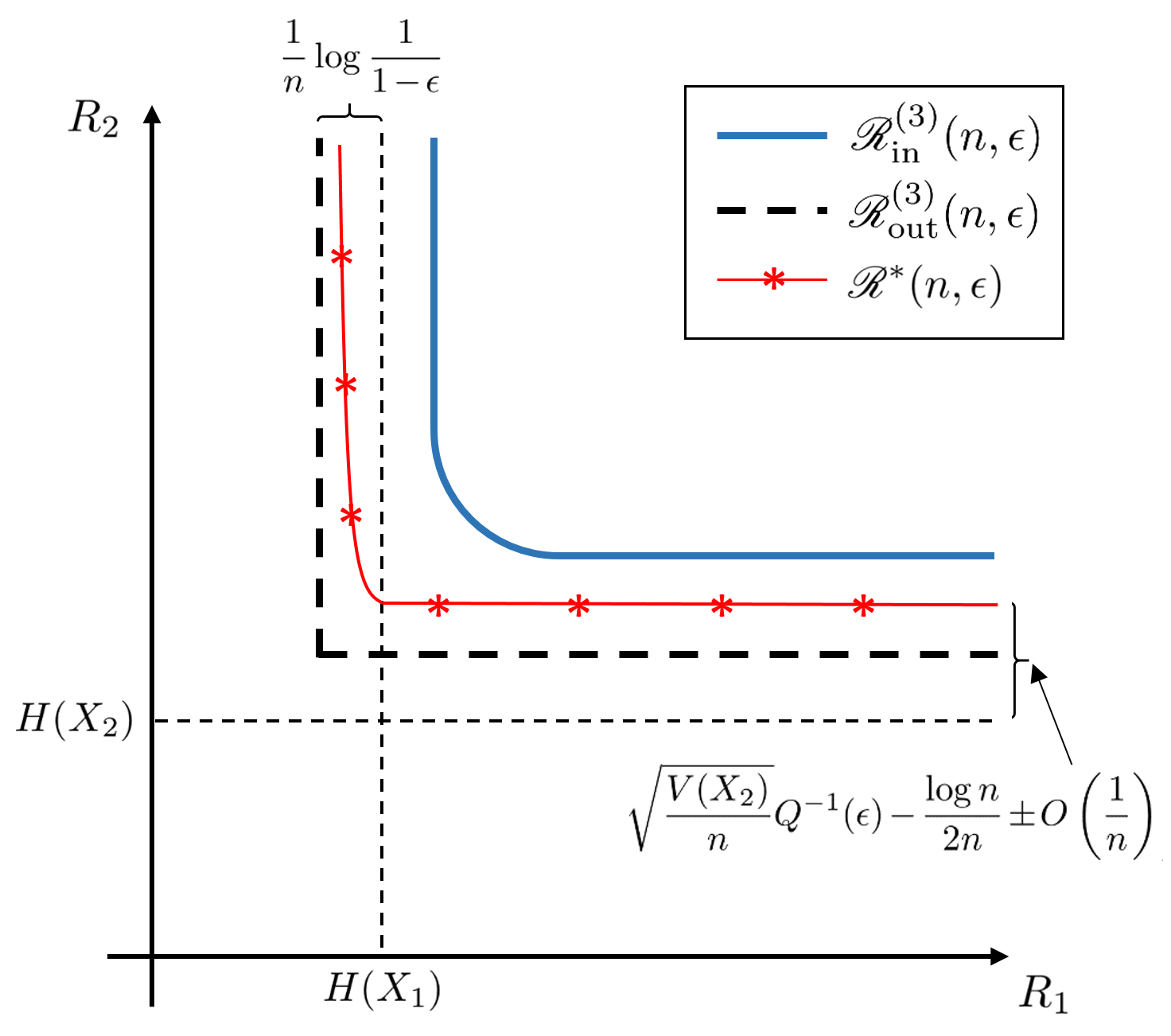 Figure 12
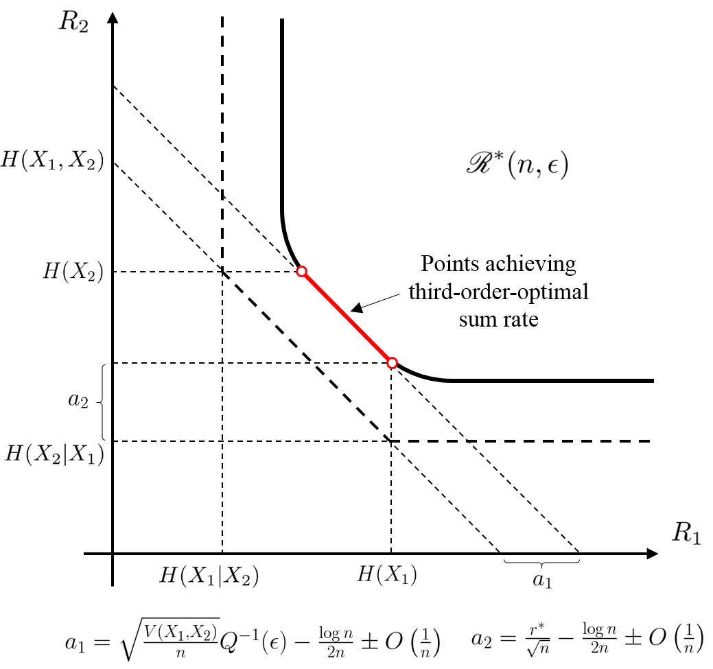 Figure 13
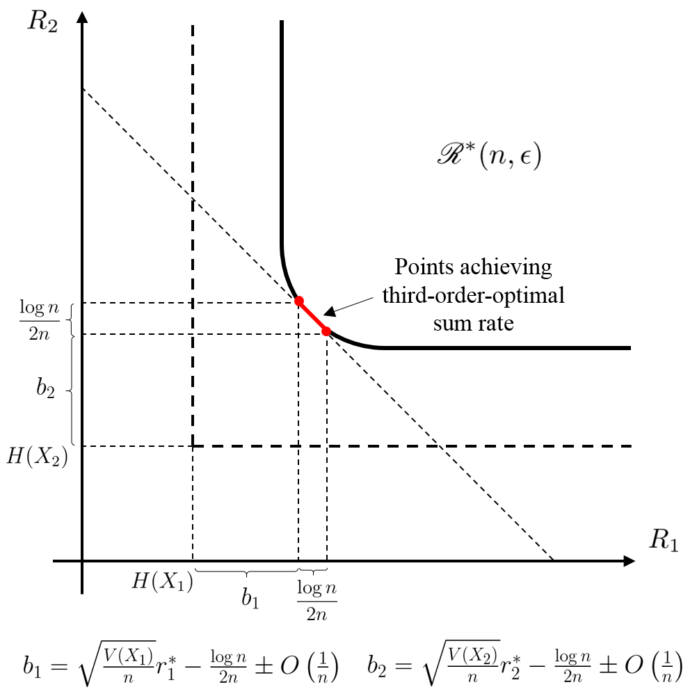 Figure 14
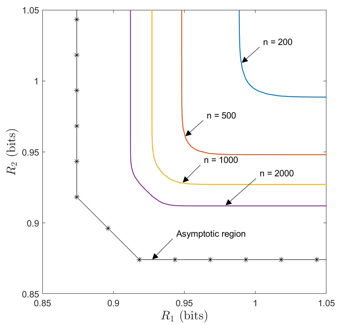 Figure 15
Peer Reviews
No public reviews on file for this paper yet. If you reviewed it on a platform where reviews are public (OpenReview, ICLR, NeurIPS, ICML), you can paste yours below so the community can read it here.
Videos
No videos yet. Explain this paper in a talk, walkthrough, or lecture? Add one.
Lossless Source Coding in the Point-to-Point,
Multiple Access, and Random Access Scenarios
Shuqing Chen, Michelle Effros, and Victoria Kostina, 1 Manuscript received September 4, 2019; revised May 27, 2020; accepted June 8, 2020This work is supported in part by the National Science Foundation under Grants CCF-1817241 and CCF-1956386. The work of S. Chen is supported in part by the Oringer Fellowship Fund in Information Science and Technology. This paper was presented in part at the 2019 IEEE International Symposium on Information Theory [1]. Matlab code for the computation of nonasymptotic bounds in this paper is available at github [2].Shuqing Chen was with the Department of Electrical Engineering, California Institute of Technology, Pasadena, CA 91125 USA. She is now with Virtu Financial Inc., New York, NY 10006 USA. (e-mail: [email protected]).Michelle Effros and Victoria Kostina are with the Department of Electrical Engineering, California Institute of Technology, Pasadena, CA 91125, USA. (e-mail: [email protected], [email protected]).Communicated by I. Kontoyiannis, Associate Editor At Large. Digital Object Identifier 10.1109/TIT.2020.3005155
Abstract
This work studies point-to-point, multiple access, and random access lossless source coding in the finite-blocklength regime. In each scenario, a random coding technique is developed and used to analyze third-order coding performance. Asymptotic results include a third-order characterization of the Slepian-Wolf rate region with an improved converse that relies on a connection to composite hypothesis testing. For dependent sources, the result implies that the independent encoders used by Slepian-Wolf codes can achieve the same third-order-optimal performance as a single joint encoder. The concept of random access source coding is introduced to generalize multiple access (Slepian-Wolf) source coding to the case where encoders decide independently whether or not to participate and the set of participating encoders is unknown a priori to both the encoders and the decoder. The proposed random access source coding strategy employs rateless coding with scheduled feedback. A random coding argument proves the existence of a single deterministic code of this structure that simultaneously achieves the third-order-optimal Slepian-Wolf performance for each possible active encoder set.
Index Terms:
Lossless source coding, Slepian-Wolf, random access, finite blocklength, random coding, non-asymptotic information theory, Gaussian approximation, hypothesis testing, meta-converse.
I Introduction
We study the fundamental limits of fixed-length, finite-blocklength lossless source coding in three scenarios:
Point-to-point: A single source is compressed by a single encoder and decompressed by a single decoder. 2. 2.
Multiple access: Each source in a fixed set of sources is compressed by an independent encoder; all sources are decompressed by a joint decoder. 3. 3.
Random access: Each active source from some set of possible sources is compressed by an independent encoder; all active sources are decompressed by a joint decoder.
The information-theoretic limit in any lossless source coding scenario is the set of code sizes or rates at which a desired level of reconstruction error is achievable. Shannon’s theory [3] analyzes this fundamental limit by allowing an arbitrarily long encoding blocklength in order to obtain a vanishing error probability. Finite-blocklength limits [4, 5, 6, 7], which are of particular interest in delay-sensitive and computationally-constrained coding environments, allow a non-vanishing error probability and study refined asymptotics of the rates achievable with encoding blocklength . Due to their non-vanishing error probability, the resulting codes are sometimes called “almost-lossless” source codes. We here use the term “source coding” to refer to this almost-lossless coding paradigm.
In point-to-point source coding, non-asymptotic bounds and asymptotic expansions of the minimum achievable rate appear in [8, 4, 9, 10, 6]. In [6], Kontoyiannis and Verdú analyze the optimal code to give a third-order characterization of the minimum achievable rate at blocklength and error probability . For a finite-alphabet, stationary, memoryless source with single-letter distribution , entropy , and varentropy ,
[TABLE]
where is the inverse complementary Gaussian distribution function, and any higher-order term is bounded by O\big{(}\frac{1}{n}\big{)}.
For a multiple access source code (MASC), also known as a Slepian-Wolf (SW) source code [11], the fundamental limit is the set of achievable rate tuples known as the rate region. The first-order rate region for stationary, memoryless and general sources appears in [11] and [12, 9], respectively. Second-order asymptotic expansions of the MASC rate region for stationary, memoryless sources appear in [13, 14]. Tan and Kosut’s characterization [13] is similar in form to the first two terms of (1), with varentropy replaced by the entropy dispersion matrix and third-order term bounded by O\big{(}\frac{\log n}{n}\big{)}.
For point-to-point source coding, our contributions include non-asymptotic characterizations of the performance of randomly designed codes using threshold and maximum-likelihood decoders. The former analysis demonstrates that combining random coding with the best possible threshold decoder cannot achieve in the third-order term in (1), and thus it is strictly sub-optimal. The latter shows that combining random coding with maximum likelihood decoding achieves the first three terms in (1). We derive both bounds by deriving and analyzing a source coding analog to the random coding union (RCU) bound from channel coding [5, Th. 16]. Our asymptotic expansion is achieved by a random code rather than the optimal code from [6]. Thus, there is no loss (up to the third-order term) due to random code design, which in turn shows that many codes have near-optimal performance; further, since our RCU bound holds when restricted to linear compressors, there are many good linear codes. The RCU bound is also important because it generalizes to the MASC and other scenarios where the optimal code is not known.
Our MASC RCU bound yields a new MASC achievability bound (Theorem 18). Establishing a link to composite hypothesis testing (HT) yields a new MASC HT converse (Theorem 19), which extends the meta-converse for channel coding in [5] to source coding with multiple encoders. This converse recovers and improves the previous converse due to Han [9, Lemma 7.2.2] and is equivalent to the LP-based converse of Jose and Kulkarni [15], which is the current best MASC converse. Our analysis of composite HT, including both non-asymptotic and asymptotic characterizations, develops tools with potential application in other multiple-terminal communication scenarios and beyond. The MASC RCU bound and HT converse together yield the third-order MASC rate region for stationary, memoryless sources (Theorem 20), revealing a third-order term that is independent of the number of encoders. This tightens the O\big{(}\frac{\log n}{n}\big{)} third-order bound from [13], which grows linearly with the source alphabet size and exponentially with the number of encoders. For dependent sources, the MASC’s third-order-optimal sum rate equals the third-order-optimal rate achievable through joint encoding.
While a MASC assumes a fixed, known collection of encoders, the set of transmitters communicating with a given access point in applications like sensor networks, the internet of things, and random access communication may be unknown or time-varying. The information theory literature treats the resulting channel coding challenges in papers such as [16, 17, 18]. We introduce the notion of a random access source code (RASC) and tackle the resulting source coding challenges. The RASC extends the MASC to scenarios where some encoders are inactive, and the decoder seeks to reliably reconstruct the sources associated with the active encoders assuming that the set of active encoders is unknown a priori.
We propose and analyze a robust RASC with rateless encoders that transmit codewords symbol by symbol until the receiver tells them to stop. Unlike typical rateless codes, which allow arbitrary decoding times [19, 20, 21, 22], our code employs a small set of decoding times. Single-bit feedback from the decoder to all encoders at each potential decoding time tells the encoders whether or not to continue transmitting.
We demonstrate (Theorem 24) that there exists a single deterministic RASC that simultaneously achieves, for every possible set of active encoders, the third-order-optimal MASC performance for the active source set. Since traditional random coding arguments do not guarantee the existence of a single deterministic code that meets multiple independent constraints, prior code designs for multiple-constraint scenarios (e.g., [21]) employ a family of codes indexed using common randomness shared by all communicators. We develop an alternative approach, deriving a refined random coding argument (Lemma 25) that demonstrates the existence of a single deterministic code that meets all our constraints simultaneously; this technique may eliminate the need for common randomness in other communication scenarios. For stationary, memoryless, permutation-invariant sources, employing identical encoders at all transmitters reduces RASC design complexity.
Except where noted, all presented source coding results apply to both finite and countably infinite source alphabets.
The organization of this paper is as follows. Section II defines notation. Section III treats (point-to-point) source coding. Section IV studies composite HT, developing general tools for multiple-encoder communication scenarios. Section V treats the MASC. Section VI introduces and studies the RASC. Each of Sections III, V, and VI follows a similar flow:
For the (point-to-point) source code: Section III-A defines the problem. Section III-B provides historical background. Section III-C presents our new random coding achievability bounds and their asymptotic expansions. 2. 2.
For the MASC: Section V-A gives definitions. Section V-B provides historical background. Section V-C presents new non-asymptotic bounds. Section V-D presents the third-order MASC characterization, comparing MASC and point-to-point source coding performance. Section V-E bounds the impact of limited feedback (and cooperation) on the third-order-optimal MASC region. 3. 3.
For the RASC: Section VI-A defines the problem and describes our proposed code. Section VI-B highlights related work. Section VI-C derives converse and achievability characterizations for our proposed code’s finite-blocklength performance. Section VI-D treats the simplified code for permutation-invariant sources.
Section VII contains concluding remarks. Proofs of auxiliary results appear in the appendices.
II Notation
For any positive integer , let . We use uppercase letters (e.g., ) for random variables, lowercase letters (e.g., ) for scalar values, calligraphic uppercase letters (e.g., ) for subsets of a sample space (events) or index sets, and script uppercase letters (e.g., ) for subsets of a Euclidean space. We use both bold face and superscripts for vectors (e.g., , , and ). Given a sequence with element in set for each and given an ordered index set , we define vector and set . Given a set , is the -fold Cartesian product of . We denote matrices by sans serif uppercase letters (e.g., ) and the -th element of matrix by . Inequalities between two vectors of the same dimension indicate elementwise inequalities. Given vector and set , denotes the Minkowski sum of and , giving . For two functions and , if there exist such that for all . For a -dimensional function , if for all . For any finite set , represents the power set of excluding the empty set, giving . We use . All uses of ‘’ and ‘’, if not specified, employ an arbitrary common base, which determines the information unit.
Denote the standard and complementary Gaussian cumulative distribution functions (cdf) by and , giving
[TABLE]
Function denotes the inverse of . The standard Gaussian probability density function is
[TABLE]
The -dimensional generalization of the Gaussian cdf is
[TABLE]
Given an ordered index set , let be a distribution defined on countable alphabet . For any with and any , the information and conditional information are defined as
[TABLE]
The corresponding entropy, conditional entropy, varentropy, conditional varentropy, third centered moment of information, and third centered moment of conditional information are defined by, respectively,
[TABLE]
We also define random variables
[TABLE]
III Point-to-Point Source Coding
III-A Definitions
In point-to-point source coding, the encoder maps a discrete random variable defined on finite or countably infinite alphabet into a message from codebook . The decoder reconstructs from the compressed description. Formal definitions of codes and their information-theoretic limits follow. For prior definitions, see, for example, [9, Chapter 1].
Definition 1** (Point-to-point source code).**
An code for a random variable with discrete alphabet comprises an encoding function and a decoding function with error probability .
Definition 2** (Block point-to-point source code).**
An code is an code defined for a random vector with discrete vector alphabet .
Definition 3** (Minimum achievable rate).**
The minimum code size and rate achievable at blocklength and error probability are defined as
[TABLE]
A discrete information source is a sequence of discrete random variables, , specified by the transition probability kernels , While Definition 2 applies to many classes of sources, including sources with memory and non-stationary sources, our asymptotic analysis focuses on stationary, memoryless sources, where for all (i.e., are i.i.d.).
III-B Background
Shannon’s source coding theorem [3] describes the fundamental limit on the asymptotic performance for lossless source coding on a stationary, memoryless source, giving
[TABLE]
In the finite-blocklength regime, Kontoyiannis and Verdú [6] characterize using upper and lower bounds that match in their first three terms and show an fourth-order gap.
Theorem 1** (Kontoyiannis and Verdú [6]).**
Consider a stationary, memoryless source with finite alphabet , single-letter distribution , and varentropy . Then111These bounds, which are stated in a base-2 logarithmic scale in [6], hold for any base. The base of the logarithm determines the information unit. (achievability) for all and all222According to [6], the achievability bound holds for any . Notice, however, that it only becomes meaningful when . ,
[TABLE]
(converse) for all and all
[TABLE]
[TABLE]
Remark 1*.*
Although [6, Theorem 1] restricts attention to and finite, the proof in [6] applies for all and any countable source alphabet, achieving the same first three terms in (1) and (19) and fourth-order term (which varies with ) provided that the third centered moment of information random variable is finite.
Remark 2*.*
When , the source is uniformly distributed over a finite alphabet (i.e., non-redundant), and . The optimal code maps any fraction of possible source outcomes to unique codewords, giving
[TABLE]
As a result, when is uniform,
[TABLE]
which matches (1) up to the second order (since ) but omits the third-order term.
Remark 3*.*
While it is not captured by our notation, is a function of . Since the third-order term appears in (1) and (19) but not in (20), the bound on , when viewed as a function of , is discontinuous at the point where equals the uniform distribution on . In contrast, , which is known and calculable, is continuous. The problem arises because Berry-Esseen type bounds are loose for small . Thus for any finite , the achievability bound in (1) blows up as . See Figure 1. Theorem 1 states that for any there exists some such that for all , behaves like in the third-order term; the smaller the value of , the larger must be.
Achievability results based on Shannon’s random coding argument [3] are important because they do not require knowledge of the optimal code, which is available only in a few special communication scenarios (e.g., [6, 7]). The following random coding achievability bound333Tighter bounds based on the optimal code appear in [9, Lemma 1.3.1] and [23, Remark 5]. is obtained by assigning source realizations to codewords independently and uniformly at random. The threshold decoder decodes to if and only if is a unique source realization that (i) is compatible with the observed codeword under the given (random) code design, and (ii) has information below .
Theorem 2** (e.g. [24], [25, Th. 9.4]).**
There exists an code for discrete random variable such that
[TABLE]
Particularizing (21) to a stationary, memoryless source with single-letter distribution satisfying and , choosing and optimally, and applying the Berry-Esseen inequality (see Theorem 6 below) gives
[TABLE]
Since the optimal application of Theorem 2 yields (22), which exceeds the bounds in Theorem 1 by in the third-order term, we are left to wonder whether random code design, threshold decoding, or both yield third-order performance penalties. In [6, Th. 8], Kontoyiannis and Verdú precisely characterize the performance of a code designed with i.i.d. uniform random codeword generation and an optimal (maximum likelihood) decoder. Unfortunately, that result is difficult to use in the asymptotic analysis. In Section III-C Theorem 4, below, we derive a new random coding bound using a maximum likelihood decoder; this result demonstrates that random coding suffices to achieve the third-order optimal performance for a stationary, memoryless source.
III-C New Achievability Bounds Based on Random Coding
We next use random code design to derive two new non-asymptotic achievability bounds for point-to-point source coding. We call these results the dependence testing (DT) bound and the random coding union (RCU) bound since they are the source coding analogues of the DT [5, Th. 17] and RCU [5, Th. 16] bounds in channel coding. The DT bound tightens Theorem 2, which is also based on threshold decoding.
Theorem 3** (DT bound).**
Given a discrete random variable , there exists an code with a threshold decoder for which
[TABLE]
Proof.
Appendix A. ∎
The proof of Theorem 3 bounds the random coding performance of a threshold decoder with threshold as
[TABLE]
where denotes a mass with respect to the counting measure on , which assigns unit weight to each . As in a channel coding argument from [5], we apply the Neyman-Pearson lemma and find that the right-hand side of (24) equals times the minimum measure of the error event in a Bayesian binary hypothesis test between with a priori probability and with a priori probability . (The Neyman-Pearson lemma generalizes to -finite measures like [23, Remark 5].) This error measure is minimized by the test that compares the log likelihood ratio to the log ratio of a priori probabilities , giving
[TABLE]
Taking minimizes the right-hand side of (24), which implies that Theorem 3 is the tightest possible bound for random coding with threshold decoding.
Particularizing Theorem 3 to a stationary, memoryless source with a single-letter distribution satisfying and and invoking the Berry-Esseen inequality (see Theorem 6 below), we obtain the asymptotic expansion
[TABLE]
Unfortunately, (25) is sub-optimal in its third-order term. Thus, random code design with threshold-based decoding fails to achieve the optimal third-order performance.
Next, we present the RCU bound, which employs random code design and maximum likelihood decoding.
Theorem 4** (RCU bound).**
Given a discrete random variable , there exists an code with a maximum likelihood decoder for which
[TABLE]
where for all .
Proof.
Our random code design randomly and independently draws encoder output for each from the uniform distribution on . We use the maximum likelihood decoder
[TABLE]
If multiple source symbols have the maximal probability mass, the decoder design chooses among them uniformly at random.
Under this random code construction, the expected error probability is bounded by the probability of event
[TABLE]
where probability measure captures both the random source output and the random encoding map . The resulting error bound is
[TABLE]
where (III-C) applies the law of iterated expectation, (III-C) bounds the probability by the minimum of the union bound and 1, (31) holds because the encoder outputs are drawn i.i.d. uniformly at random and independently of , and (32) rewrites (31) in terms of the distribution .
The existence of the desired code follows since (32) equals the right-hand side of (26). ∎
Remark 4*.*
By the argument employed in the proof of [25, Th. 9.5], we obtain the same RCU bound if we randomize only over linear encoding maps. Thus, there is no loss in performance when restricting to linear compressors.
We next show that the RCU bound recovers the first three terms of the achievability result in Theorem 1. Thus, the sub-optimal third-order terms in (22) and (25) result from the sub-optimal decoder rather than the random encoder design. This is important since optimal codes are not available for scenarios like the MASC studied in Section V, below.
Theorem 5 focuses on a stationary, memoryless source with single-letter distribution satisfying
[TABLE]
Define constants
[TABLE]
where is the absolute constant in the Berry-Esseen inequality for i.i.d. random variables. (See Theorem 6, below.)
Theorem 5** (Third-order-optimal achievability via random coding).**
Consider a stationary, memoryless source satisfying the conditions in (33) and (34). For all ,
[TABLE]
where \xi(n)=O\big{(}\frac{1}{n}\big{)} is bounded more precisely as follows.
For all and ,
[TABLE] 2. 2)
For all and ,
[TABLE]
Before we show our proof of the asymptotic expansion in Theorem 5, we state two auxiliary results used in our analysis. The first is the classical Berry-Esseen inequality (e.g., [26, Chapter XVI.5]), stated here with the best known absolute constant from [27].
Theorem 6** (Berry-Esseen inequality).**
Let be independent random variables such that and . Then for any real and ,
[TABLE]
where ( for identically distributed ) [27].
We refer to as the Berry-Esseen constant.
The second result is from Polyanskiy et al. [5, Lemma 47].
Lemma 7** ([5, Lemma 47]).**
In the setting of Theorem 6, it holds for any and that
[TABLE]
Proof of Theorem 5.
We analyze the RCU bound of Theorem 4 for random variable . For notational brevity, define
[TABLE]
By Theorem 4, there exists an code such that
[TABLE]
where , and each of and is a sum of i.i.d. random variables. Applying Lemma 7 with and gives
[TABLE]
Plugging (44) in (43), we find
[TABLE]
where (46) plugs (44) into (43), (46) separates the cases and , and (47) applies Lemma 7 to the second term in (46).
Denote for brevity
[TABLE]
We now choose
[TABLE]
and apply the Berry-Esseen inequality (Theorem 6) to (47), giving and proving achievability bound
[TABLE]
To obtain (37) from (49), we note that as long as ,
[TABLE]
where (51) applies the definition of the Gaussian cumulative distribution function and its complement from (2) and (3), (52) holds by a first-order Taylor bound for some , and (53) holds by the inverse function theorem.
- For and , and is decreasing in . We can further bound the right-hand side of (53) and conclude that
[TABLE]
- For and , we have and is increasing in . We conclude that
[TABLE]
Plugging (54) and (55) into (49) gives (38) and (39). ∎
IV Composite Hypothesis Testing
The meta-converse for channel coding [5, Th. 26]444The quantum information theory literature contains an earlier approach to channel coding converses using binary hypothesis testing [28], [29, Ch. 4.6]. and its generalizations to lossy source coding [23] and joint source-channel coding [30, 31] apply binary hypothesis testing to derive converses in point-to-point communication problems. To extend this approach to multi-terminal coding (see, e.g., Section V Theorem 19, below), we develop a corresponding method using composite hypothesis testing. We first develop non-asymptotic tools and then analyze the asymptotics.
A composite hypothesis test tests a simple hypothesis against a composite hypothesis:
[TABLE]
where is the observation, is the distribution under the simple hypothesis, and is the collection of possible distributions under the composite hypothesis. The following definition generalizes the optimal -function from binary to composite hypothesis testing. (See, for example, [32, Def. 1].)
Definition 4**.**
The set of achievable false-positive errors for power- tests between distribution and collection of distributions is the subset of defined as
[TABLE]
where denotes a probability with respect to , and for each , denotes a probability with respect to .
Like binary hypothesis tests (see [23, Remark 5]), composite hypothesis tests can be generalized to allow and to be -finite measures; in such cases, may not be a subset of . We apply this generalization in Section V-C2 to derive our new MASC converse.
In [32], Huang and Moulin study the asymptotics of the set , giving a third-order-optimal characterization [32, Th. 1]. As noted in [33, Appendix D], there is a gap in their converse proof (see also Remark 6, below). We here present a comprehensive analysis of composite hypothesis testing, starting with non-asymptotic characterizations and then particularizing them to give a new proof of [32, Th. 1].
IV-A Non-Asymptotic Bounds
The analysis of in [32] uses the test that achieves the minimal (boundary) points of that set. For each minimal point , there exists a vector , , such that the generalized Neyman-Pearson test
[TABLE]
achieves ; here is chosen so that . While the above test is optimal, the achievability and converse bounds that follow simplify the asymptotic analysis.
Lemma 8** (Achievability).**
For any , , there exists a composite hypothesis test for which
[TABLE]
Proof.
Fix any , . Consider the (sub-optimal) likelihood-ratio threshold test555In [32], Huang and Moulin also use this sub-optimal likelihood-ratio threshold in their asymptotic achievability analysis.:
[TABLE]
Under this test, (58) follows immediately, and (8) holds by
[TABLE]
∎
The following converse bound extends [5, Eq. (102)] from binary hypothesis testing to composite hypothesis testing.
Lemma 9** (Converse).**
For any , if , then
[TABLE]
where , are arbitrary constants.
Proof.
Appendix B. ∎
Lemma 10 extends the argument of [34, Lemma 1] from binary to composite hypothesis testing.
Lemma 10** (Variational lemma).**
For any , if , then
[TABLE]
where , , are arbitrary constants and equality is achieved by a generalized Neyman-Pearson test.
Proof.
Appendix C. ∎
Given any , define
[TABLE]
Then Lemma 10 gives
[TABLE]
Remark 5*.*
We can derive Lemma 9 from the variational characterization in Lemma 10 by noting that
[TABLE]
Lemmas 9 and 10 are useful beyond the asymptotic analysis of composite hypothesis testing. They also make it possible to recover previous converse bounds from our new MASC meta-converse, as presented in Section V-C2 below.
IV-B Asymptotics for I.I.D. Distributions
We here characterize the asymptotics of when each of and is a product of identical single-shot distributions, i.e., and , .
We begin with notation. For each , define
[TABLE]
Define vector and matrix as
[TABLE]
Let be a Gaussian random vector with mean zero and covariance matrix . Define the multidimensional counterpart of the function as
[TABLE]
The set appears in characterizations such as [13, 32]. When is non-singular, the boundary of approaches in each dimension , as illustrated in Figure 2LABEL:sub@fig-sve-1. For , lies in the positive orthant of ; for , extends outside of the positive orthant. If , then . See Figure 2LABEL:sub@fig-sve-2 for plots of the boundaries of in . If is singular with rank , then lies in an -dimensional subspace of .
Theorem 11 derives a third-order-optimal characterization of under assumptions
[TABLE]
Define the inner and outer bounding sets
[TABLE]
where vector and matrix are defined in (75) and (76).
Theorem 11** (Third-order-optimal asymptotics).**
Assume that and are product distributions composed of identical single-shot distributions that satisfy (78) and (79). For any , the set satisfies
[TABLE]
where .
Remark 6*.*
In [32, Th. 1], Huang and Moulin claim the third-order-optimal result in Theorem 11 when is non-singular. Unfortunately, there is a gap in their converse proof. Applying [32, Lemma 2] to get [32, Eq. (13)] requires that vector is independent of . However, they consider any , which may grow with because set is unbounded. Thus, [32, Eq. (13)] does not always hold.
We resolve this issue with a new proof of Theorem 11 that leverages Lemmas 8 and 9. We first show two auxiliary results.
The multidimensional Berry-Esseen theorem bounds the probability of a sum of i.i.d. random vectors. Bentkus’ theorem [35, Th. 1.1] for the case with mean zero and identity covariance achieves the best known dependence on dimension. Tan and Kosut extend [35, Th. 1.1] to non-singular covariance matrices [13, Cor. 8]. We here extend [13, Cor. 8] to covariance matrices with non-zero rank.
Lemma 12**.**
Let be i.i.d. random vectors in with mean zero and covariance matrix . Let be a Gaussian vector in . Define . Let be a matrix whose columns are the normalized eigenvectors of with non-zero eigenvalues. Define i.i.d. random vectors such that for . Let and . If , then for all ,
[TABLE]
where is the smallest eigenvalue of matrix .
Proof.
Appendix D. ∎
If , then and Lemma 12 recovers [13, Cor. 8].
The following lemma is useful for our asymptotic analysis.
Lemma 13**.**
Fix an arbitrary positive-semidefinite matrix and . Then, the following results hold.
There exist constants and such that for all ,
[TABLE] 2. 2.
There exist constants and such that for all ,
[TABLE]
Proof.
Appendix E. ∎
Proof of Theorem 11.
Define random variables
[TABLE]
and random vector
[TABLE]
For brevity, denote
[TABLE]
To prove the achievability part of Theorem 11, we particularize Lemma 8 to product distributions and to obtain that for any , there exists a test for which
[TABLE]
Take any such that
[TABLE]
where is the constant on the right side of (81) for , which is finite under assumptions (78) and (79). Applying Lemma 12 to (87) gives
[TABLE]
where and matrix is defined in (76). Applying Lemma 7 to (88) gives
[TABLE]
where
[TABLE]
is a finite positive constant by the assumptions in (78) and (79). Plugging (89) into (93) and noting (92) gives
[TABLE]
where (96) follows from Lemma 13-82.
For the converse, recall from Lemma 9 that if , then any must satisfy
[TABLE]
for all , . Take
[TABLE]
Then, (97) becomes
[TABLE]
where (100) applies Lemma 12 and is the constant in the right side of (81). By the definition of in (77), (100) implies that
[TABLE]
Applying Lemma 13-83, we conclude from (101) that
[TABLE]
∎
V Multiple Access Source Coding
To simplify notation, we focus on MASCs with two encoders. Our definitions and results generalize to more than two encoders, as briefly noted in Remark 12 below.
V-A Definitions
In a MASC [11], also known as a Slepian-Wolf source code, independent encoders compress a pair of random variables with discrete alphabets and . Encoder , , observes only , which it maps to a codeword in ; a single decoder jointly decodes the pair of codewords to reconstruct . We first define codes for abstract random objects and then particularize to random objects that live in an alphabet endowed with a Cartesian product structure.
Definition 5** (MASC).**
An MASC for random variables with discrete alphabets and comprises two encoding functions and and a decoding function, with error probability .
In block coding, encoders individually observe and drawn from distribution on . Our block MASC definition is similar to those in [13] and [14].
Definition 6** (Block MASC).**
An MASC is an MASC for random vectors on . The code rate is given by
[TABLE]
Definition 7** (-rate region).**
Rate is -achievable if there exists an MASC with and . The -rate region is the closure of the set of -achievable rate pairs.
While definitions 6 and 7 apply to arbitrary discrete random variables , , with transition probability kernels , our asymptotic analysis focuses on stationary, memoryless sources, where for all
For any rate and distribution , define
[TABLE]
V-B Background
In [11], Slepian and Wolf prove that if are stationary and memoryless, then for every ,
[TABLE]
(i.e., the strong converse holds). We call this region the asymptotic MASC rate region.
In [12], Miyake and Kanaya give achievability and converse bounds for finite-blocklength coding on finite-alphabet sources. In [9], Han gives corresponding results for sources with countable alphabets. While these results are stated in [9] for general sources whose alphabets adopt -fold Cartesian product structures, we here describe them in an abstract form.
Theorem 14** (Achievability, Han [9, Lemma 7.2.1]).**
Given discrete random variables , there exists an MASC satisfying
[TABLE]
where is an arbitrary constant.
Theorem 15** (Converse, Han [9, Lemma 7.2.2]).**
Any MASC on discrete random variables satisfies
[TABLE]
where is an arbitrary constant.
In [15], Jose and Kulkarni derive a new linear programming (LP) finite-blocklength converse, tightening the bound in Theorem 15 with an extra non-negative term (see [15, Cor. 13]).
Theorem 16** (LP-based converse, [15, Th. 12]).**
Any MASC on discrete random variables satisfies
[TABLE]
where the supremum is over such that for all .
The best prior asymptotic expansion of the MASC rate region is the second-order characterization developed independently in [13, 14]. In [13], Tan and Kosut introduce an entropy dispersion matrix, which serves a role similar to the scalar dispersion in the point-to-point case [5, 6, 23].
Definition 8** (Tan and Kosut [13, Def. 7]).**
The entropy dispersion matrix for random variables is the covariance matrix of random vector
[TABLE]
Note that is a positive-semidefinite matrix with , , and on the diagonal.
Tan and Kosut [13] give a second-order characterization of the MASC rate region for finite-alphabet stationary, memoryless sources in terms of the asymptotic rate region and the entropy dispersion matrix. Their result, reproduced below, exhibits an O\big{(}\frac{\log n}{n}\big{)} gap in the third-order term.
Define
[TABLE]
where and are defined in (104), is the entropy dispersion matrix for (Definition 8), , and is the absolute finite positive constant from [13, Def. 6].
Theorem 17** (Tan and Kosut [13, Th. 1]).**
Consider finite-alphabet, stationary, memoryless sources with for every . For any and all sufficiently large,
[TABLE]
Remark 7*.*
The inner boundary defined in (LABEL:eq-sw-tk-1) is achievable by a universal coding scheme [13, Sec. VI]. The outer bounding region in (LABEL:eq-sw-tk-2) is based on [9, Lemma 7.2.2].
In [14], Nomura and Han use [9, Lemma 7.2.1] and [9, Lemma 7.2.2] to derive a second-order MASC coding theorem for stationary, memoryless, dependent sources. Their result is equivalent to Theorem 17 up to the second-order term and applies also for countable alphabets. Neither [13] nor [14] finds the precise third-order term. In Sections V-C and V-D, below, we give new non-asymptotic MASC bounds and then apply them to precisely characterize the third-order asymptotics.
V-C New Non-Asymptotic Bounds
V-C1 Achievability
We present a MASC RCU bound, extending Theorem 4 to the multiple-encoder case.
Theorem 18** (MASC RCU bound).**
Given discrete random variables , there exists an MASC with
[TABLE]
where
[TABLE]
Proof.
For every , , draw i.i.d. uniformly at random from . The maximum likelihood decoder is defined for each by
[TABLE]
where ties are broken equiprobably at random in the code design. This decoder is optimal for the given encoder.
We bound the random code’s expected error probability by the probability of the union of events
[TABLE]
By a derivation similar to that in the proof of Theorem 4,
[TABLE]
and (124) is equal to the right side of (113) as desired. ∎
Figure 4 in Section V-D1 plots the point-to-point (Theorem 4) and MASC (Theorem 18) RCU bounds.
V-C2 Converse
The MASC composite hypothesis testing converse employs the set (see Definition 4) and its generalization to -finite measures.
Theorem 19** (Hypothesis testing (HT) converse).**
Let be the source distribution defined on . Let , , and be any -finite measures defined on . Any MASC satisfies
[TABLE]
where
[TABLE]
Proof.
Consider an MASC with stochastic encoders and and stochastic decoder , where and are the encoder outputs, and is the decoder output. Fix distributions on . Then Z=1\big{\{}(\hat{X}_{1},\hat{X}_{2})=({X}_{1},{X}_{2})\big{\}} defines a (sub-optimal) composite HT for testing against , for which and
[TABLE]
where (130) follows since is independent of , and (131) follows by bounding the probability in the sum over by 1. Similarly,
[TABLE]
[TABLE]
Thus (19) holds by the definition of . ∎
To recover Han’s converse (Theorem 15) from Theorem 19, let and be the marginals of and let , , and be the counting measures over , , and . By Theorem 19, any MASC satisfies
[TABLE]
Applying Lemma 9 to (136) with gives
[TABLE]
Setting , , and for an arbitrary recovers Theorem 15.
To show that Theorem 19 is equivalent to the LP-based converse (Theorem 16), we apply (IV-A) to Theorem 19, showing that any MASC satisfies
[TABLE]
The outer supremum is over -finite measures , , and . In Appendix F, we show that the bounds in (138) and (108) are equivalent, establishing the equivalence between the MASC HT (Theorem 19) and LP (Theorem 16) converses.
Remark 8*.*
When one of the sources is deterministic, the MASC HT converse reduces to the point-to-point HT converse [23, Eq. (64)]. For example, if is deterministic, then (136) reduces to
[TABLE]
which further reduces to
[TABLE]
where is the optimal -function for binary hypothesis testing between distributions and .
V-D Asymptotics: Third-Order MASC Rate Region
The following third-order asymptotic characterization of the MASC rate region for stationary, memoryless sources closes the O\big{(}\frac{\log n}{n}\big{)} gap between (LABEL:eq-sw-tk-1) and (LABEL:eq-sw-tk-2).
Consider stationary, memoryless sources with single-letter joint distribution for which
[TABLE]
When (139) holds666In fact, the weaker condition , , suffices., . Technical assumptions (139), (140), and (141) are required to ensure applicability of the multidimensional Berry-Esseen theorem and Lemma 7 in our asymptotic analysis. Assumption (140) is satisfied automatically if the alphabets and are finite.
Define the set
[TABLE]
where vector is defined in (104), is the entropy dispersion matrix for , and is defined in (77). Note that (see Definition 7) but . Define the inner and outer bounding sets
[TABLE]
Theorem 20** (Third-order MASC rate region).**
Consider a pair of stationary, memoryless sources with single-letter joint distribution satisfying (139)–(141). For any , the -rate region satisfies
[TABLE]
Since the upper and lower bounds in Theorem 20 agree up to their third-order terms, we call the third-order MASC rate region. Figure 3 plots the boundaries of at different values of for an example pair of sources.
Remark 9*.*
As noted in Remark 2, for point-to-point source coding, zero varentropy means that the source is uniform; the third-order term is absent in that case. While condition (139) limits Theorem 20 to sources with positive varentropies, Appendix G considers the case where one or more varentropies are zero. Roughly, each zero varentropy yields a zero dispersion, and the absence of a third-order term, similar to the point-to-point case. Furthermore, if but , the corresponding achievable third order term increases from to [math].777This is seen by modifying the reasoning in (172)–(187) in the proof of Theorem 20 below. This means that the optimal third order term lies in in that case.
Proof of Theorem 20: achievability.
We apply Theorem 18 to stationary, memoryless sources with and then apply Lemmas 7 and 12 to analyze the bound. Let
[TABLE]
where , , are drawn i.i.d. according to the joint distribution defined in (18). With this notation, the random variables , , defined in (114), (115), (116) particularize as
[TABLE]
By Theorem 18, there exists an MASC such that
[TABLE]
To bound each of the terms in (157), we first bound the random variables , , and by random variables , , and that are easier to work with.
Denote constants
[TABLE]
that are finite by assumptions (139) and (140). Define
[TABLE]
for . Define and for analogously.
Applying Lemma 7 to yields
[TABLE]
To bound , we consider the cases and separately. If , then
[TABLE]
is finite by assumption (140), and Lemma 7 yields
[TABLE]
If , then irrespective of the realization of , and
[TABLE]
Putting (165) and (166) together yields
[TABLE]
Similarly,
[TABLE]
where is defined analogously to (164).
Next, we apply Lemma 7 again to further bound each of the first three terms in (157):
[TABLE]
We proceed to bound the last term in (157). For fixed constants and , define the events and that and are typical, respectively:
[TABLE]
Note that
[TABLE]
where
[TABLE]
are both finite by the assumptions in (139) and (140).
Applying the union bound to , , and Chebyshev’s inequality
[TABLE]
to both terms, we observe that for each ,
[TABLE]
where
[TABLE]
are finite by assumption (141).
We are now prepared to apply Lemma 12 to the last term in (157). Pick any pair of rates satisfying
[TABLE]
where the set is defined in (142), , and is the Bentkus constant in the right-side of (81) for zero-mean i.i.d. random vectors
[TABLE]
Note that by assumption (140). We have
[TABLE]
where (185) applies (174) and , and (187) applies (182), Lemma 12 and (179).
Substituting (169), (170), (171), and (187) into (157) yields , and the proof is complete since the set of satisfying (182) contains by Lemma 13-82. ∎
Proof of Theorem 20: converse.
We invoke Theorem 19 with , , , and , where and are the marginals of , and , , and are the counting measures over , , and . Applying Theorem 11 to under the assumptions in (139) and (140), we conclude that in order to attain error probability , and must satisfy
[TABLE]
which is equivalent to (144), as desired. ∎
Remark 10*.*
The converse of Theorem 20 can also be proved using Han’s converse (Theorem 15) with and Lemmas 12 and 13 in a way similar to that in the achievability proof above, except that we would use Lemma 13 to bound \mathscr{Q}_{\rm inv}\left(\mathsf{V},\epsilon+O\left(\frac{1}{\sqrt{n}}\right)\big{)}\subseteq\mathscr{Q}_{\rm inv}(\mathsf{V},\epsilon)-O\left(\frac{1}{\sqrt{n}}\right)\right)\mathbf{1} instead of . Our HT converse (Theorem 19) is stronger than Han’s converse, but the gap is in the fourth- or higher-order terms, as illustrated through computation in Figure 4. Han’s achievability bound (Theorem 14) with the third-order optimal choice of leads to the third order term of instead of . Thus Han’s achievability is weaker than our RCU bound (Theorem 18) in the third order term.
Remark 11*.*
Tan and Kosut’s converse (Theorem 17) is also based on Han’s converse. Instead of deriving an outer bound on as given in Lemma 13, they apply the multivariate Taylor approximation to expand the probability, giving a bound that is loose in the third-order term.
Remark 12*.*
Theorem 20 generalizes to any finite number of encoders. Let be a nonempty ordered set with a unique index for each encoder. For any vector , define the -dimensional vector of its partial sums as
[TABLE]
For any distribution defined on and any , define -dimensional vectors
[TABLE]
and entropy dispersion matrix
[TABLE]
for random vector . Define set
[TABLE]
Thus, while . Finally,
[TABLE]
If every element of has a positive variance and a finite third centered moment, then for any ,
[TABLE]
V-D1 Comparison with Point-to-Point Source Coding
Figure 4 compares joint (point-to-point) compression of to the MASC sum-rate at the symmetrical rate point (). The gap between the MASC and point-to-point HT converses captures a penalty due to separate encoding. For small , the third-order Gaussian approximation (without the term) is more accurate at than at since the term blows up as approaches [math].
It is well-known that optimal MASCs incur no first-order penalty in achievable sum rate when compared to joint coding [11, 12, 9]. We next investigate the higher-order penalty of the MASC’s independent encoders.
Tan and Kosut introduce a quantity known as the local dispersion [13, Def. 4] to characterize the second-order speed of convergence to any asymptotic MASC rate point from any direction. For any non-corner point on the diagonal boundary of the asymptotic MASC rate region, the sum rate’s second-order coefficient is optimal when approached either vertically or horizontally. Approaching corner points incurs a positive second-order penalty relative to point-to-point coding.
Two corollaries of Theorem 20, below, bound the MASC penalty by considering the achievable sum rate for different choices of and . We treat the cases where and are dependent and and are independent separately, assuming throughout that (139) and (140) hold.
When and are dependent, , and the asymptotic sum-rate boundary contains non-corner and corner points. Corollary 21, below, shows that a MASC incurs no first-, second-, or third-order performance penalty relative to joint coding at non-corner points (i.e., when and ); in contrast, a MASC suffers a second-order performance penalty at corner points (i.e., when or ). See Figure 5LABEL:sub@fig-sw-sumrate-1 for an illustration.
Corollary 21**.**
Suppose that and are dependent.
Fix constants and . Then there exists some constant such that if
[TABLE]
then for all . 2. 2.
Fix . If
[TABLE]
*for some , then . Conversely, if , then *
[TABLE]
where is the solution to equation
[TABLE]
and is the covariance matrix for random vector .
Proof.
Appendix H. ∎
For independent sources, the asymptotic sum-rate boundary contains only the single (corner) point , and the entropy dispersion matrix
[TABLE]
is singular.
The next result concerns the third-order-optimal sum rate
[TABLE]
According to Theorem 20, characterizes the best achievable sum rate in SW source coding up to an gap.
Corollary 22**.**
For independent and ,
[TABLE]
which is achieved by with
[TABLE]
for any and
[TABLE]
Proof.
Appendix I. ∎
By Corollary 22, for independent sources a unique captures the best MASC second-order sum-rate; the third-order term is achieved at all points on a segment of the rate region boundary. See Figure 5LABEL:sub@fig-sw-sumrate-2. Under assumption (139),
[TABLE]
where for independent. Here (208) follows since its left-hand side solves
[TABLE]
and the constraint in (209) requires and , which gives the bound since
[TABLE]
Therefore, when and are independent, a MASC incurs a positive second-order sum-rate penalty relative to joint coding. Closed-form expressions for this penalty are available in special cases. When , , and the penalty is
[TABLE]
When and are i.i.d., the penalty equals the penalty for coding a vector of i.i.d. outputs from by applying an independent (point-to-point) code with error probability to each of and instead of a single code to vector .
V-E Limited Feedback and Cooperation
The RASC proposed in Section VI employs limited feedback. We here analyze the impact of feedback on the underlying MASC. In our feedback model, the decoder broadcasts the same bits of feedback to both encoders. A bit sent at time must be a function of the encoder outputs received in time steps . (See Figure 6LABEL:sub@fig-fb.) We bound the impact of feedback by studying a MASC with a *cooperation facilitator (CF).*888The CF is introduced for multiple access channel coding in [36] and extended to source and network coding in [37]. The CF broadcasts the same -bit function of the sources to both encoders prior to their encoding operations. (See Figure 6LABEL:sub@fig-cf.) Since the MASC network has no channel noise, feedback from the decoder cannot convey more information than feedback from the CF. As a result, we bound the impact of feedback by bounding the impact of cooperation, which is easier to work with in our analysis.
We begin by defining the CF-MASC and its rate region.
Definition 9** (CF-MASC).**
An CF-MASC for random variables on comprises a CF function , two encoding functions and , and a decoding function given by
[TABLE]
with error probability
[TABLE]
Definition 10** (Block CF-MASC).**
An MASC is a CF-MASC for random variables on .
The code’s finite blocklength rates are defined by
[TABLE]
Definition 11** (-CF rate region).**
A rate pair is -CF achievable if there exists an CF-MASC with , , and . The -CF rate region is defined as the closure of the set of all -CF achievable rate pairs.
We use to denote the feedback-MASC (FB-MASC) rate region, which is defined as the closure of the set of all -achievable rate pairs when the same bits of feedback from the decoder are available to both encoders.
Since the CF sees the source vectors while the decoder sees a coded description of those vectors (using a deterministic code), an -bit CF can implement any function used to determine the decoder’s -bit feedback. As a result, any rate point that is achievable by an -bit FB-MASC is also achievable by an -bit CF-MASC. Therefore, for any and ,
[TABLE]
Theorem 23 bounds CF-MASC (and FB-MASC) performance, showing that for any , the third-order rate region for -bit CF-MASCs cannot exceed the corresponding MASC rate region. Hence finite feedback does not enlarge the third-order MASC rate region. This result generalizes to scenarios with more than two encoders.
Theorem 23** (CF-MASC Converse).**
Consider stationary, memoryless sources with single-letter distribution satisfying (139) and (140). For any and ,
[TABLE]
Thus and share the same outer bound.
Proof.
Appendix J. ∎
Remark 13*.*
The same proof can be used to show that allowing to grow as does not change the first three terms in the optimal characterization of the -MASC.
Remark 14*.*
For dependent sources, the optimal third-order MASC sum rate equals the optimal third-order sum rate with full cooperation. (See the discussion in Section V-D1, above.). Since even an infinite amount of decoder feedback is weaker than full cooperation, an infinite amount of feedback does not improve the third-order sum rate in this case.
VI Random Access Source Code (RASC)
An RASC is a generalization of an MASC for networks where the set of participating encoders is unknown to both the encoders and the decoder a priori. We begin by defining the problem and describing our proposed communication strategy.
VI-A Definitions and Coding Strategy
Let be the maximal number of active encoders. We associate each encoder with a unique source from the set of sources indexed by . Each encoder chooses whether to be active or silent. Only sources associated with active encoders are compressed and reconstructed. By assumption, the decision to remain silent is independent of the observed source instance. Given the joint distribution on countable alphabet , when ordered set of is active, the marginal on the transmitted sources is
[TABLE]
Thus, each encoder’s state has no effect on the statistical relationship among sources observed by other encoders.
As in the random access channel code from [18], our proposed RASC organizes communication into epochs. At the beginning of each epoch, each encoder independently decides its activity state; that activity state remains unchanged until the end of the epoch. Thus, the active encoder set is fixed in each epoch. Each active encoder observes source output and independently maps it to a codeword comprised of a sequence of code symbols from alphabet . The codewords are sent simultaneously to the decoder. Since set is unknown a priori, the encoder behavior cannot vary with . The decoder sees and decides a time , called the decoding blocklength, at which to jointly decode all received partial codewords. The set of potential decoding blocklengths is part of the code design; it is known to all encoders and to the decoder.
Figure 7 illustrates our coding scheme in one epoch when . Each encoder sends a single code symbol per time step. At each time , the decoder sends a “0” to indicate that it is not yet ready to decode; at time , the decoder sends a “1,” ending one epoch and starting the next. The decoder then reconstructs source vector using the first code symbols from each active encoder. To avoid wasting time in an epoch with no active encoders, we include decoding time in set . The decoder sends at most bits of feedback, and encoders need only listen for decoder feedback at the times in set .
To formalize the above strategy, fix . Define vectors
[TABLE]
with and .
Definition 12** (RASC).**
An RASC for sources on source alphabet comprises a collection of encoding and decoding functions
[TABLE]
where is the encoding function for source and is the decoding function for active coder set . For each , source vector is decoded at time with error probability \mathbb{P}\big{[}\mathsf{g}_{\mathcal{T}}\left(\mathsf{f}_{i}(X_{i})_{[m_{\mathcal{T}}]},i\in\mathcal{T}\right)\neq\mathbf{{X}}_{\mathcal{T}}\big{]}\leq\epsilon_{\mathcal{T}}, where denotes the first code symbols of .
Definition 13 particularizes Definition 12 to the block setting.
Definition 13** (Block RASC).**
An RASC is an RASC for an -block of source outcomes. The parameter , called the encoding blocklength does not vary with .
An RASC behaves, for each , like a \big{(}(Q_{i}^{m_{\mathcal{T}}},\,i\in\mathcal{T}),\epsilon_{\mathcal{T}}\big{)} MASC (see Definition 5) with a finite number of feedback bits. However, the RASC is one code. Its descriptions are nested (i.e., for each , if , then is a prefix of ). It simultaneously satisfies the error constraints for all . And, since the code symbol alphabet sizes are fixed, its rate vectors are coupled. See Figure 8.
The following definitions build toward the non-asymptotic fundamental limit of RASCs.
Definition 14** **(-Valid and -Rate
sets).
A collection of rate vectors is -valid if s.t.
[TABLE]
The set is the set of -valid rate collections. The collection is -achievable if there exists an RASC. The -rate set is the set of -achievable rate collections.
VI-B Background
While the concept of an RASC is new, the RASC problem is related to the universal MASC problem. Like a universal MASC, the RASC is designed for an unknown distribution from a known collection of possible distributions. In this case, the possible distributions are . The RASC differs, however, from universal MASCs since even the set of active encoders is unknown a priori.
A short summary of prior universal MASCs follows.
For a fixed-rate MASC and finite source alphabets, universal decoding can be realized using type methods. (See [13], [38], [39].) Such strategies achieve optimal performance only when the source’s MASC rate region matches the code’s fixed rate. 2. 2.
Oohama [40] and Jaggi and Effros [41] study the effect of limited encoder cooperation on the asymptotically universally achievable rate region. Rate-zero cooperation between encoders suffices to achieve universality in the asymptotic regime. Oohama characterizes the optimal error exponents in [40]. 3. 3.
Yang et al. [42] study a block MASC with progressive encoding; the code uses zero-rate feedback to universally achieve the asymptotic MASC rate region. Sarvotham et al. [43] propose a variable-rate block sequential coding scheme with zero-rate feedback for binary symmetric sources, showing that at blocklength and target error probability , the backoff from the asymptotic MASC rate due to universality is . 4. 4.
In [22], Draper introduces a rateless MASC with single-bit feedback. Draper’s algorithm asymptotically achieves the optimal coding rates for sources with unknown joint distributions but known finite alphabet sizes. See [44] for a practical rateless MASC.
VI-C Asymptotics: Third-Order Performance of the RASC
In this section, we analyze the performance of an RASC for stationary, memoryless sources. Results include both achievability and converse characterizations of the -rate set under the assumption that the single-letter joint source distribution satisfies
[TABLE]
Constraints (221)–(223) enable us to use Berry-Esseen bounds. The resulting characterization is tight up to the third-order term. While the existence of an RASC implies the existence of an \big{(}n,(Q_{i}^{m_{\mathcal{T}}},\,i\in\mathcal{T}),\epsilon_{\mathcal{T}}\big{)} MASC for each , the existence of individual MASCs does not imply the existence of a single RASC that simultaneously satisfies the error probability constraints for all possible configurations of active encoders. Indeed, the existence of a single RASC that simultaneously performs as well (up to the third-order term) as the optimal MASC for each is one of our most surprising results.
Define the inner and outer bounding sets
[TABLE]
where and are the third-order MASC bounding sets for distribution . (See (194) and (LABEL:eq-def-sw-out).)
Theorem 24** (Third-order RASC performance).**
For any , consider stationary, memoryless sources specified by a single-letter joint distribution satisfying (221)–(223). For any ,
[TABLE]
The converse and achievability proofs follow.
Proof of Theorem 24: converse.
As shown in Section V-E (Theorem 23), even with a priori knowledge of the encoder set and bits of feedback, a MASC for the encoders in set cannot achieve performance outside of the third-order MASC outer bounding set . ∎
The achievability part of Theorem 24 provides a sufficient condition for the existence of a single RASC that is simultaneously good for all . To prove this, we first derive an achievability result assuming that the encoders and decoder share the common randomness used to generate a random code (Theorem 26). Unfortunately, the existence of a random code ensemble with expected error probability satisfying the error probability constraint for each does not guarantee the existence of a single deterministic code satisfying those constraints simultaneously. We therefore take a different approach, which, unexpectedly, combines a converse bound on error probability and a random coding argument to show achievability.
The following refinement of the random coding argument provides a bound on the probability (with respect to the random code choice) that the error probability of a randomly chosen code exceeds a certain threshold. The code of interest here can be any type of source or channel code.
Lemma 25**.**
Let be any class of codes with a corresponding error probability for each . Let
[TABLE]
denote the error probability of the best code in . Then any random code ensemble999A random code ensemble is a random variable defined on code set . defined over satisfies
[TABLE]
Proof.
Let be any non-negative random variable and define ; that is, is the largest constant for which almost surely. By Markov’s inequality,
[TABLE]
Taking and yields the desired result. ∎
In the regime of interest . Therefore, the right side of (228) is decreasing as a function of , and replacing by any converse on yields a valid achievability bound. Thus Lemma 25 provides a means to leverage a converse to prove achievability.
Given any RASC , for each let denote the error probability of code under active encoder set . The RASC achievability proof applies Lemma 25 with error probability for each . Before proceeding to that proof, we use Theorem 26, below, to define a random code ensemble and calculate its expected error probability.
Theorem 26** (Random code).**
For any , consider a source distribution defined on countable alphabet . There exists a random code ensemble defined on the set of all RASCs with decoding blocklengths and code alphabets for which the following inequalities hold simultaneously for all :
[TABLE]
where
[TABLE]
and the expectation in (231) is with respect to the conditional distribution
[TABLE]
Proof.
We construct the random code ensemble as follows.
Random Encoding Map: For every , draw encoder outputs for all i.i.d. uniformly at random from , where .
Maximum Likelihood Decoder: For any , , and , denote the first symbols of by . For each , the maximum likelihood decoder for observes the first symbols from the encoders in , here denoted by
[TABLE]
and, for each , produces the output
[TABLE]
Expected Error Analysis: The expected error probability over the random code ensemble is bounded above by the probability of event
[TABLE]
It follows that
[TABLE]
and (239) is equal to the right-hand-side of (26). Here, (239) considers the case where source symbols in set are decoded incorrectly for each . The derivation of (239) from (239) follows the argument in (124)–(124). Specifically, since each component of differs from the corresponding component of and since the encoder output for each is drawn independently and uniformly at random from ,
[TABLE]
for any . ∎
We now prove the achievability part of Theorem 24 by applying Lemma 25 to the random code in Theorem 26.
Proof of Theorem 24: achievability.
The probability that random RASC has error probability greater than for some possible set of active encoders is
[TABLE]
To bound each term using Lemma 25, we next bound the expected error probability and the error probability for the best code in , where is the set of \big{(}n,(Q_{i}^{m_{\mathcal{T}}},\,i\in\mathcal{T}),\epsilon_{\mathcal{T}}\big{)} MASCs with set as in (248) below.
To find , we apply Theorem 26 to our stationary, memoryless sources with -symbol distribution . Given any and , let
[TABLE]
Under moment assumptions (221)–(223), one can generalize the argument in (146)–(186) to active encoders to obtain
[TABLE]
where , and are finite positive constants.
Fix any . By the definition of in (189) and the relation in (220), we see that
[TABLE]
For brevity, define constant vector
[TABLE]
and the almost-constant error thresholds
[TABLE]
where is the Bentkus constant (81) for the vector of information densities (243). We choose the decoding blocklength as
[TABLE]
where (which may be a function of ) satisfying will be determined in the sequel, and is defined in (193). Applying Lemma 12 to (244) with in (248) yields
[TABLE]
To lower-bound , for each and define
[TABLE]
where is the -MASC rate region (see Remark 12), is defined in (LABEL:eq-def-sw-out), and (251) is by the converse (Theorem 23). By Lemma 13-83, one can always choose such that for sufficiently large
[TABLE]
It follows that
[TABLE]
Equation (253) and the converse (Theorem 23) imply that the minimal error probability over satisfies
[TABLE]
Plugging (249) and (254) into Lemma 25 and noting the monotonicity of the bound in Lemma 25 gives
[TABLE]
We may choose to ensure that the right-hand side of (256) is as small a constant as desired. Specifically, we choose constants to satisfy
[TABLE]
and put
[TABLE]
With (256) and (258), we bound the right-hand side of (242) as
[TABLE]
which implies the existence of a deterministic RASC with in (248), in (245), and in (248). ∎
Remark 15*.*
When parameters are fixed, increasing yields larger decoding blocklengths . Therefore, the choice of to satisfy (257) controls the RASC performance trade-off across different active encoder sets. This trade-off affects the performance of the RASC in the fourth- or higher-order terms.
VI-D RASC for Permutation-Invariant Sources
A permutation-invariant101010Polyanskiy [17] introduces a similar notion of permutation invariance for multiple access channel coding in [17]. source is defined by the constraint
[TABLE]
for all permutations on and all . For example, given any and , the marginal of satisfies (260). Such “hidden variable” models have applications in statistics, science, and economics, where latent variables (e.g., the health of the world economy or the state of the atmosphere) influence observables (e.g., stock prices or climates). Figure 9 shows an example with sensors reading measurements of a common hidden state .
Permutation-invariant source models interest us both because of their wide applicability and because they present an opportunity for code simplification through identical encoding, where all encoders employ the same encoding map. For any permutation-invariant source, (215) and (260) imply that for all and, for any with ,
[TABLE]
Thus, is permutation-invariant for every and the joint source distribution depends on the number of active encoders but not their identities. Assuming that we further employ the same error probability for all with , we can fix a single decoding blocklength for each number of active encoders and use identical encoders at all transmitters, allowing us to accommodate an arbitrarily large number of encoders without designing a unique encoder for each. A similar phenomenon arises for RA channel coding [18].
In analyzing RASC performance with identical encoders on a permutation-invariant source, we assume in addition to (221) and (222) that no two sources are identical, i.e.,
[TABLE]
This is important since using identical encoders on identical sources yields identical descriptions, in which case descriptions from multiple encoders are no better than descriptions from a single encoder. Under these assumptions, Theorem 24 continues to hold. In the analysis, we modify the decoder to output the most probable source vector that contains no repeated symbols (see the proof of Theorem 26), treating the case where contains repeated symbols as an error. In the asymptotic analysis for stationary, memoryless sources, the probability of this error event is bounded by
[TABLE]
which decays exponentially in by (262). Therefore, under the assumption in (262), identical encoding does not incur a first-, second-, or third-order performance penalty.
VII Concluding Remarks
This paper studies finite-blocklength lossless source coding in three scenarios.
We derive a new non-asymptotic achievability (RCU) bound (Theorem 4) and use it to show that for point-to-point coding on stationary, memoryless sources, random code design with maximum likelihood decoding achieves the same coding rate up to the third-order as the optimal code from [6]. The RCU bound generalizes to the MASC scenario (Theorem 18).
A new HT converse (Theorem 19) extends the channel coding meta-converse [5] to an MASC and suggests the possibility of using composite hypothesis testing to derive converses for other multi-terminal scenarios. Our analysis of composite hypothesis testing provides general tools (Lemmas 8, 9, and 10) for use in other related problems. Just as the meta-converse for channel coding recovers previously known converses, our HT converse recovers Han’s MASC converse [9, Lemma. 7.2.2]. Just as the HT converse for lossy source coding [23, Th. 8] is equivalent to the LP-based converse for that setting (see [15, Cor. 3]), our MASC HT converse is equivalent to the MASC LP-based converse [15, Th. 12].
We give the first third-order characterization of the MASC rate region for stationary, memoryless sources, tightening prior second-order characterizations from [13] and [14] and replacing the thresholds used there to decode for users by a maximum likelihood decoder that chooses the jointly most probable source realizations consistent with the received codewords. We show that for rate points converging to a non-corner point on the asymptotic sum-rate boundary, separate encoding does not compromise the performance in lossless data compression up to the third-order term. Numerical comparison of the new HT converse and the optimal performance of point-to-point source coding in Figure 4 allows one to bound from below the small gap between joint and separate encoding, which is not captured in the first three terms of the asymptotic expansion. For independent sources, there are no non-corner points, and MASC separate encoding incurs a positive penalty in the second-order term relative to joint encoding with a point-to-point code. When two sources have the same marginals, this penalty equals the penalty for using two independent blocklength- codes rather than a single blocklength- point-to-point code for encoding samples.
Our proposed RASC works universally for all possible encoder activity patterns. The nested structure of the RASC demonstrates that there is no need for the encoders to know the set of active encoders a priori. The third-order-optimal MASC performance is achievable even when the only information the encoders receive is the acknowledgment that tells them when to stop transmitting (Theorem 24).
Our refinement of the traditional random coding argument (Lemma 25 and (242)) uses bounds on the minimal (converse) and expected (achievability) error probabilities for each possible active encoder set to show the existence of a single code that is good for all possible active encoder sets. This argument is likely to be useful for other information-theoretic problems.
Appendix A Proof of Theorem 3
Following [5, Eq. (68)], note that for and
[TABLE]
Let and . Then taking the expectation of both sides of (A.1) with respect to gives
[TABLE]
where denotes a probability with respect to and denotes a mass with respect to the counting measure on , which assigns unit weight to each . In light of (A.2), we can prove (23) by demonstrating the existence of an code for which the right-hand side of (A.2) exceeds . We prove a slightly stronger result, showing that there exists an code with a threshold decoder such that
[TABLE]
for all . Setting in (A.3) yields the desired bound.
Fix . For each , randomly and independently draw each encoder output from the uniform distribution on . Define the threshold decoder
[TABLE]
We capture all errors using a union of error events
[TABLE]
By the random coding argument and the union bound, there exists an code such that
[TABLE]
Here,
[TABLE]
where (A.10) applies the union bound and (A.11) holds since the encoder outputs are i.i.d. and uniformly distributed. ∎
Appendix B Proof of Lemma 9
The proof extends the proof of [5, Eq. (102)] (e.g., [24]). We show that for any test that decides between vs. ,
[TABLE]
where , are arbitrary constants. Then Lemma 9 follows immediately by definition of .
To prove (B.1), fix a for each . We then have
[TABLE]
where (B.4) follows from the non-negativity of probability and each . The proof is complete since (B.7) equals the right-hand-side of (B.1). ∎
Appendix C Proof of Lemma 10
For any test deciding between vs. , we show that
[TABLE]
where , are arbitrary constants. Fix a for each . For notational brevity, define sets
[TABLE]
For any test , we have
[TABLE]
The equality in (C.7) is achieved by test
[TABLE]
for any . Rearranging (C.8) yields (C.1). Choosing the unique to satisfy , we obtain Lemma 10 by the definition of . ∎
Appendix D Proof of Lemma 12
Recall that is composed of the normalized eigenvectors corresponding to the non-zero eigenvalues of covariance matrix V and , where for . Thus , where is non-singular.
For each , define
[TABLE]
which is a convex subset of . Let . Applying [13, Cor. 8] to the i.i.d. random vectors , we obtain
[TABLE]
which is equivalent to (81) by the definition of . ∎
Appendix E Proof of Lemma 13
For simplicity, we assume that is non-singular. When is singular, a similar analysis can be applied with replaced by defined in Lemma 12.
Let be a -dimensional multivariate Gaussian with covariance matrix . Recall from (77) that is defined as
[TABLE]
By the definition of and the definition of in (II), if and only if lies on the boundary of , and if and only if lies in the interior of .
Proof of Lemma 13.
To prove (82), consider any and . Since is continuously differentiable everywhere provided that is non-singular, we can apply the multivariate Taylor’s theorem to expand as
[TABLE]
The second-order residual term can be bounded as
[TABLE]
where
[TABLE]
and denotes the max norm of a matrix.
Denote
[TABLE]
Since is increasing in any coordinate of , . Then, for any , we have
[TABLE]
We note that for any finite positive , approaches as . Thus, for any finite positive that satisfies , there exists some such that for all ,
[TABLE]
which yields
[TABLE]
By the definitions of and , (E.9) implies
[TABLE]
and consequently
[TABLE]
which proves (82).
Eq. (83) can be proved in a similar way.
∎
Appendix F Equivalence between HT and LP-Based Converses for the MASC
In this appendix, we establish the equivalence between the HT converse and the LP-based converse by showing that the bounds in (108) and (138) are equivalent. According to [15, Eq. (31)], (108) is equivalent to the following converse
[TABLE]
where the supremum is over
[TABLE]
Therefore, we show that (F.1) is equivalent to (138).
We first demonstrate that (F.1) implies (138). Set
[TABLE]
for any -finite and , . Since
[TABLE]
To prove the other direction, we substitute , , and in the right-hand side of (138) to obtain
[TABLE]
Take a supremum of the right-hand side of (F.3) over . Since (F.3) does not contain , this does not change anything. Now, weaken (i.e., lower-bound) the inner supremum over by setting
[TABLE]
Observing that
[TABLE]
we see that the result of our weakening is exactly the right-hand side of (F.1), as desired. ∎
Appendix G MASCs for Sources with Less Redundancy
Applying Lemma 7 to get the asymptotic achievability result in Theorem 20 requires that all , , and are strictly positive (as an implication of assumption (139)). Thus, the analysis in Section V-D breaks down when any of these varentropies is equal to zero. (We refer to such a source as being less redundant.) In this appendix, we analyze the performance of the MASC for less redundant sources. Specifically, we consider a pair of stationary, memoryless sources and analyze the following three cases:
all three varentropies are equal to zero; 2. 2)
exactly two of the varentropies are equal to zero; 3. 3)
exactly one of the varentropies is equal to zero.
We continue to assume that the joint distribution satisfies (140) and (141). For those cases in which , we continue to assume . Likewise, if , we continue to assume .
In point-to-point almost-lossless source coding, the optimal code for a non-redundant source is easy to find (see Remark 2). When the encoders are required to operate independently in a MASC, we know no easy way to find the optimal codes in general. In Section A below, we give characterizations of the -rate region in the three general cases listed above using the techniques developed in Section V-D. Then, in Section B, we restrict attention to the case where for every ; under this condition, the optimal codes can be found and analyzed directly.
G-A General Characterizations of the -Rate Region
We first list our results in the three general cases below.
Case 1): Suppose that , , and . For any , , , let
[TABLE]
Define
[TABLE]
Theorem 27**.**
When , , and , the -rate region satisfies
[TABLE]
As in the point-to-point scenario, there are no second-order dispersion terms or third-order terms in the characterization of in this case. For any and , the achievable region has a curved boundary due to the trade-off in the fourth-order terms, while the converse region has three linear boundaries.
Case 2): There are three possible cases where exactly two of the three varentropies are equal to zero. Here, we suppose that while . The other two cases can be analyzed in the same way. Let denote the Berry-Esseen constant for the random variable , and let , , be the finite positive constants defined in (181), (158), and (176), respectively. For any , , , let
[TABLE]
Define
[TABLE]
Theorem 28**.**
When , , and , the -rate region satisfies
[TABLE]
The achievable region has a curved boundary due to the trade-off in , , and . If we let
[TABLE]
then it is apparent that the dispersion corresponding to is with a third-order term, while the dispersions of and are zero.
Case 3): Similar to Case 2), there are three possible cases where exactly one of the three varentropies is equal to zero. Here, we consider the case where while and . Let , , , and be the finite positive constants defined in (180), (159), (177), and (160), respectively, and let be the Bentkus constant (81) for the vector . For any , let
[TABLE]
where , and is the covariance matrix of the random vector . Define
[TABLE]
Theorem 29**.**
When , , and , the -rate region satisfies
[TABLE]
For any and , the achievable region has a curved boundary that is characterized by the trade-off between a separate bound on and a region in that bounds jointly. The converse region is the intersection of a region with a linear boundary that bounds only and a region with a curved boundary that bounds jointly. If we let
[TABLE]
then it is apparent that the dispersion corresponding to and is given by with a third-order term, while the dispersion of is zero.
A less redundant stationary, memoryless source has some useful properties. When ,
[TABLE]
for every ; in other words, is uniformly distributed over its support in . When ,
[TABLE]
in other words, is uniformly distributed over its conditional support for each . When , a result analogous to (G.16) holds. These properties do not reduce the difficulty of characterizing the optimal MASCs in general. As a result, we continue to employ the random coding techniques from Section V-D in our analysis here. For the achievability argument, we invoke the MASC RCU bound (Theorem 18); for the converse, we appeal to a modified version of [9, Lemma 7.2.2], as stated below.
Lemma 30** (Modified [9, Lemma 7.2.2]).**
Any MASC satisfies
[TABLE]
for any , , , where , and are defined in (146)–(148).
We next prove Theorems 27, 28, and 29.
Proof of Theorem 27.
Achievability: We employ the RCU bound in (155). To evaluate the terms in (155), note that the uniformity over the distribution’s support that results from implies that for any such that ,
[TABLE]
Similar equalities hold for and , and for any , (155) gives
[TABLE]
implying that such a rate pair is achievable. Therefore, the -rate region satisfies
[TABLE]
Converse: Consider any with . Since the bound in (30) holds for any , , , we take
[TABLE]
which, under the given uniformity, implies
[TABLE]
We take and sufficiently large so that
[TABLE]
and hence
[TABLE]
Under these conditions, (30) gives
[TABLE]
Therefore, any achievable rate pair must satisfy
[TABLE]
The same analysis applies to and . We then conclude that any achievable rate pair must satisfy . Thus,
[TABLE]
∎
Proof of Theorem 28.
Achievability: Take (G.6) satisfying the inequalities in (G.5) with some , , such that . We again employ the RCU bound from (155). Since , we use (174) to bound . The terms and are constants (cf. (G.18)). With these observations, we weaken (156) as
[TABLE]
where (G.30) is by our choice of , and (G.31) applies (169), the Berry-Esseen inequality (Theorem 6), and (179) to bound the three probability terms. Therefore, is achievable at blocklength and error probability , implying
[TABLE]
Converse: We next apply Lemma 30 to derive a converse result. Recall that under our assumptions , and almost surely. Consider any such that . Since the bound in (30) holds for any , , , we can take
[TABLE]
so that
[TABLE]
By this choice of , . Thus, we can take and sufficiently large such that
[TABLE]
By the above choices of , , and , (30) gives
[TABLE]
Therefore, any achievable rate pair must satisfy
[TABLE]
The same analysis applies to , and we conclude that any achievable rate pair must also satisfy
[TABLE]
Given (G.37) and (G.38), we re-evaluate the bound in (30) by taking
[TABLE]
Under these conditions, we have
[TABLE]
and the bound in (30) becomes
[TABLE]
Then, by the Berry-Esseen inequality (Theorem 6), taking
[TABLE]
in (G.41) yields . Therefore, any achievable rate pair must satisfy . Thus,
[TABLE]
∎
Proof of Theorem 29.
Achievability: Take any satisfying the inequalities in (G.10) with some . We employ the RCU bound in (155). Since and , we use (175) and (163) to bound and , respectively; is the constant in (G.18). With these observations, we weaken (156) as
[TABLE]
where (G.45) is by our choice of , and (G.46) applies (170), (171), Lemma 12 (multidimensional Berry-Esseen Theorem), and (179) to bound the four probability terms. Therefore, is achievable at blocklength and error probability , implying that
[TABLE]
Converse: We employ Lemma 30 to derive a converse. Recall that in this case, almost surely. Consider any such that . Since the bound in (30) holds for any , , , we can set
[TABLE]
so that
[TABLE]
By this choice of , . Thus, we can take and sufficiently large such that
[TABLE]
By the above choices of , , and , (30) gives
[TABLE]
Therefore, any achievable rate pair must satisfy
[TABLE]
Given that (G.52) holds, we re-evaluate the bound in (30) by taking
[TABLE]
Under these conditions, the bound in (30) becomes
[TABLE]
Applying Lemmas 12 and 13 to (G.54), we conclude that any in the -rate region must satisfy . Thus,
[TABLE]
∎
G-B Two Special Cases
The analysis in Section G-A above applies to any stationary, memoryless source with single-letter distribution that satisfies (140). In such a general setting, it is hard to find an optimal code. However, there are some special cases in which the optimal codes for a less redundant source can be characterized.
To enable the following analysis on these special cases, we assume that for every . Under this assumption, if and only if . As a result, the three cases discussed in Section A reduce to only two possible scenarios:
; 2. 2)
, and either or .
Note that and are independent in both of these scenarios.
We first summarize the results below.
Special Case 1):
Theorem 31**.**
Suppose that , , and . If satisfies for every , then
[TABLE]
where is defined in (G.3).
This scenario is a special example of Case 1) discussed in Section A above. The -rate region here coincides with the converse region presented in (G.3) for general source distributions. See Figure 10LABEL:sub@fig-sw-1 for a comparison among , , and in this special case.
Special Case 2): With , we here assume that and . The other case can be analyzed similarly. For any , we define
[TABLE]
where the functions and are characterized as follows. For any fixed , and . For any fixed , both and blow up as approaches . (These bounds are applications of the point-to-point results in Theorem 1.) Also define
[TABLE]
Theorem 32**.**
Suppose that , , and . If satisfies for every , then
[TABLE]
This scenario is a special example of Case 3) discussed in Section A of this appendix. The -rate region characterized in (G.61) is sandwiched between the achievable region presented in (G.11) and the converse region presented in (G.12). To compare these regions, we note that the bounds on in (G.11) and (G.12) become inactive in this special scenario where and are independent. As a result, the achievable region in (G.11) becomes
[TABLE]
and the converse region in (G.12) becomes
[TABLE]
As approaches , the boundary of the -rate region given in (G.59) approaches the line , which matches the vertical segment of the boundary of the converse region . See Figure 10LABEL:sub@fig-sw-2 for a comparison of , , and in this case.
We next give proofs for Theorems 31 and 32.
Proof of Theorem 31.
When , is uniformly distributed over , which restricts and to be finite and and to be independent. The MASC problem reduces to independent (point-to-point) almost-lossless source coding problems for the two sources with a single compound error probability. As a result, the optimal MASC with blocklength and code sizes has an error probability given by
[TABLE]
Therefore, for any , there exists an MASC if and only if
[TABLE]
In this case, and .
For and , (G.65) becomes
[TABLE]
which is equivalent to
[TABLE]
For , (G.65) becomes
[TABLE]
which is equivalent to
[TABLE]
For , (G.65) gives
[TABLE]
For all and ,
[TABLE]
∎
Proof of Theorem 32.
When and , is uniformly distributed over , which implies that is finite and . In contrast, is not uniform over . Moreover, and are independent. The MASC problem in this case can also be resolved via independent point-to-point source coding for each of the two sources. The optimal code with blocklength and code sizes encodes arbitrary symbols in and a cardinality- subset of that has the largest probability with respect to . As a result, for any , there exists an MASC if and only if
[TABLE]
where is the total marginal probability of symbols that are not encoded in , and is the total marginal probability (with respect to ) of the encoded symbols in . Eq. (G.72) implicitly requires and .
For , we have
[TABLE]
In this case, (G.72) gives
[TABLE]
We can apply the point-to-point almost-lossless source coding results from Theorem 1 to obtain
[TABLE]
For , we have
[TABLE]
In this case, (G.72) gives
[TABLE]
We can also apply the point-to-point results to get
[TABLE]
where for any fixed , and ; for any fixed , both and blow up as approaches (see Theorem 1 for the case where approaches [math]). ∎
Appendix H Proof of Corollary 21
[TABLE]
Define
[TABLE]
We have
[TABLE]
Let be a multivariate Gaussian in , where is the entropy dispersion matrix (see Definition 8). Then
[TABLE]
where (H.7) holds by the union bound. It follows that
[TABLE]
where (H.10) applies the Chernoff bound of the Q-function, and (H.11) holds since . Similarly,
[TABLE]
In contrast,
[TABLE]
Plugging (H.11)–(H.13) into (H.7), we conclude that for all sufficiently large such that
[TABLE]
the bound
[TABLE]
holds. Therefore, , and hence (142).
- Recall vector defined in (H.3). With ,
[TABLE]
Note that
[TABLE]
Since , decays exponentially in . Therefore, by the definition of in (202) and a first-order multivariate Taylor bound, in (200) can be chosen so that the right side of (H.19) is equal to , which implies that (142).
Conversely, for any such that ,
[TABLE]
which further implies
[TABLE]
Thus, by the definition of ,
[TABLE]
which is equivalent to (201). ∎
Appendix I Proof of Corollary 22
Fix any . Define
[TABLE]
By the assumption that and are independent, we have
[TABLE]
Denote
[TABLE]
Let be a multivariate Gaussian in , where is the entropy dispersion matrix of the independent sources and . It follows in this case that and are independent and . We then have
[TABLE]
Thus, for any , such that
[TABLE]
and hence
[TABLE]
Therefore,
[TABLE]
On the other hand, for any , such that
[TABLE]
and hence (142). Thus, (I) holds with equality.
Appendix J Proof of Theorem 23
The proof employs an extension of Han’s MASC converse [9, Lemma 7.2.2].
Given an CF-MASC , let
[TABLE]
Then equals the code’s error probability, and
[TABLE]
where the bound on is the number of distinct decoder inputs and the bounds on and are the number of distinct decoder inputs under fixed values of and and an -bit CF. Fix . Define sets
[TABLE]
Then,
[TABLE]
where (J) follows the definition of , (J.8) applies , and (J.9) holds by (J.2). Similarly,
[TABLE]
Thus,
[TABLE]
Rearranging (J.13) gives a lower bound on the error probability . Thus, any CF-MASC must satisfy
[TABLE]
Particularizing (J.14) to stationary, memoryless sources with single-letter distribution satisfying (139) and (140) shows that any CF-MASC must satisfy
[TABLE]
where is an arbitrary constant, , , and are defined in (146), (147), and (148), and is defined in (183). Let be a finite constant that does not grow with and let . Applying Lemma 12 and Lemma 13-83 to bound the probability (J.16) in a manner similar to (182)–(187), we conclude that any -achievable rate pair must be in (144). ∎
Remark 16*.*
One could also prove Theorem 23 by extending our HT converse (Theorem 19 ) to the setting with a cooperation facilitator. Our Theorem 19 continues to hold with and replaced by and in (126) and (127), respectively ((128) remains unchanged).
Acknowledgment
The authors would like to thank the anonymous reviewer for the especially careful review that is reflected in the final version.
The reference list from the paper itself. Each links out to its DOI / PubMed record.
- 1[1] S. Chen, M. Effros, and V. Kostina, “Lossless source coding in the point-to-point, multiple access, and random access scenarios,” in Proc. IEEE Int. Symp. Inf. Theory (ISIT) , Jul. 2019, pp. 1692–1696.
- 2[2] SPECTRE: Short packet communication toolbox. [Online]. Available: https://github.com/yp-mit/spectre/tree/master/lossless-sc
- 3[3] C. E. Shannon, “A mathematical theory of communication,” The Bell System Technical Journal , vol. 27, no. 2, pp. 379–423 and 623–656, July and Oct. 1948.
- 4[4] V. Strassen, “Asymptotische abschäzungen in shannons informationstheorie,” in Proc. Trans. Third Prague Conf. Inf. Theory, Statist., Decision Funct., Random Process. , 1964, pp. 689–723.
- 5[5] Y. Polyanskiy, H. V. Poor, and S. Verdú, “Channel coding rate in the finite blocklength regime,” IEEE Trans. Inf. Theory , vol. 56, no. 5, pp. 2307–2359, May 2010.
- 6[6] I. Kontoyiannis and S. Verdú, “Optimal lossless data compression: Non-asymptotics and asymptotics,” IEEE Trans. Inf. Theory , vol. 60, no. 2, pp. 777–795, Feb. 2014.
- 7[7] V. Kostina, Y. Polyanskiy, and S. Verdú, “Variable-length compression allowing errors,” IEEE Trans. Inf. Theory , vol. 61, no. 8, pp. 4316–4330, Aug. 2015.
- 8[8] A. A. Yushkevich, “On limit theorems connected with the concept of entropy of Markov chains,” Uspekhi Mat. Nauk , vol. 8, no. 5(57), pp. 177–180, 1953.