Peculiarities in the gravitational field of a filamentary ring
Daniel Schumayer, David A. W. Hutchinson

TL;DR
This paper analyzes the gravitational field of a filamentary ring, providing an analytic potential expression, exploring its unique properties, and identifying conditions for stable, periodic orbits outside the ring.
Contribution
It offers the first analytic expression for the gravitational potential of a filamentary ring and investigates its dynamical properties and orbit stability.
Findings
The gravitational potential is not central, highlighting differences between center of mass and gravity.
Only the z-component of angular momentum is conserved due to symmetry.
Stable, periodic orbits exist outside the ring if angular momentum exceeds a threshold.
Abstract
The gravitational field of a massive, filamentary ring is considered. We provide an analytic expression for the gravitational potential and demonstrate that the exact gravitational potential and its gradient, thus the gravitational force-field, is not central. Hence it is a good candidate to discuss the difference between the concepts of center of mass and center of gravity. We focus on other consequences of reduced symmetry, e.g., only the -component of the angular momentum is conserved. However, the remnant high symmetry of this system also ensures that there are special classes of motions which are restricted to invariant subspaces, thus, depending on the initial condition, the dynamics of a point particle is integrable. We also show that periodic orbits in the equatorial plane external to the ring are possible, but only if the angular momentum is above a threshold value. In this…
Click any figure to enlarge with its caption.
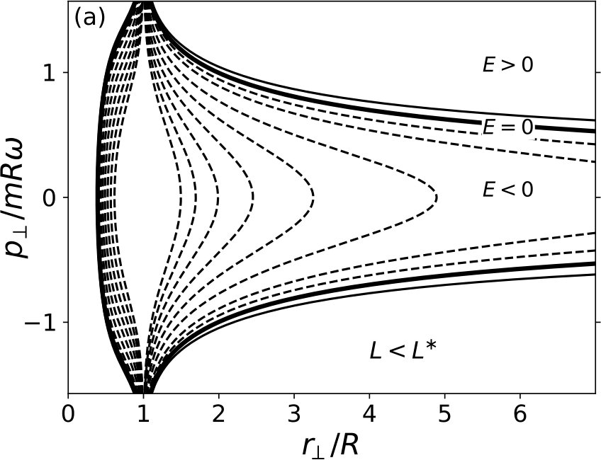 Figure 10
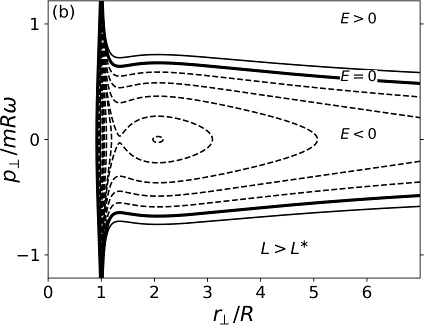 Figure 11
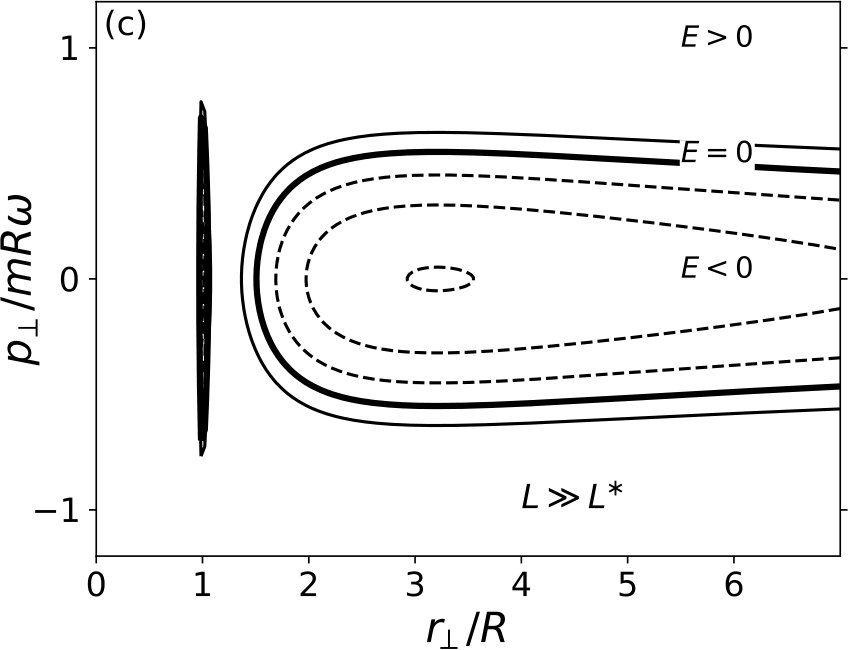 Figure 12
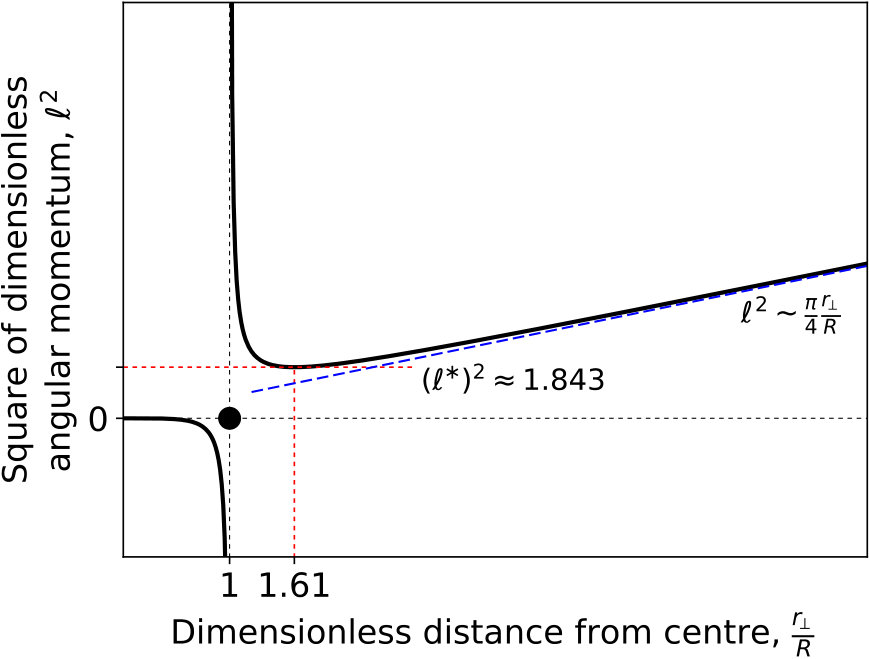 Figure 13
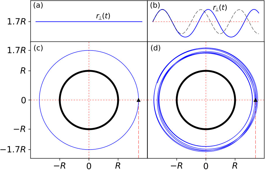 Figure 14
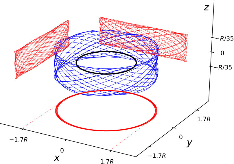 Figure 15
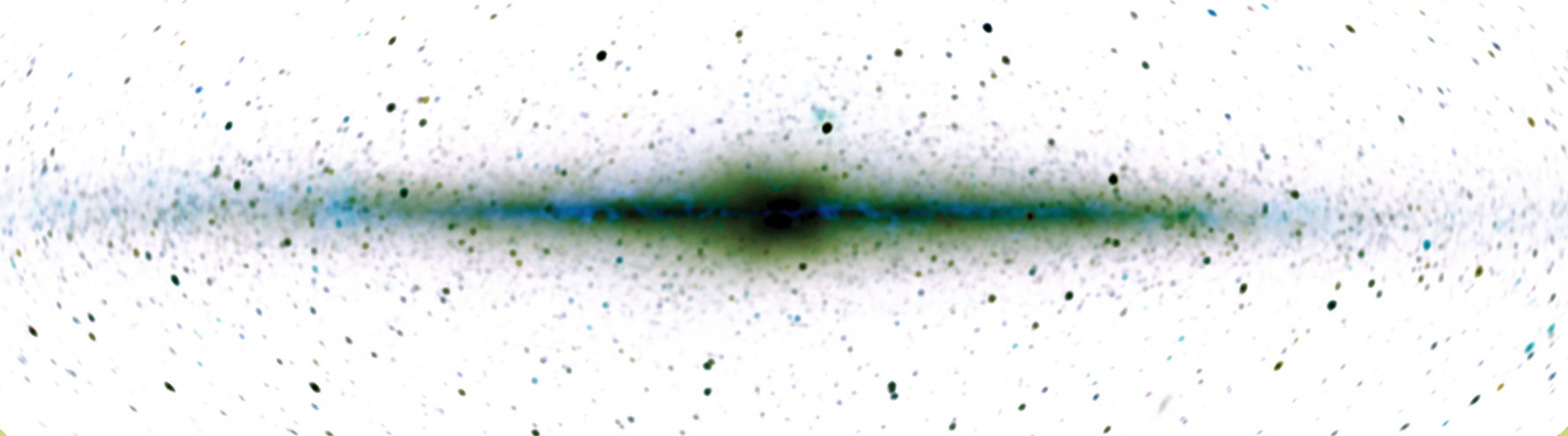 Figure 1
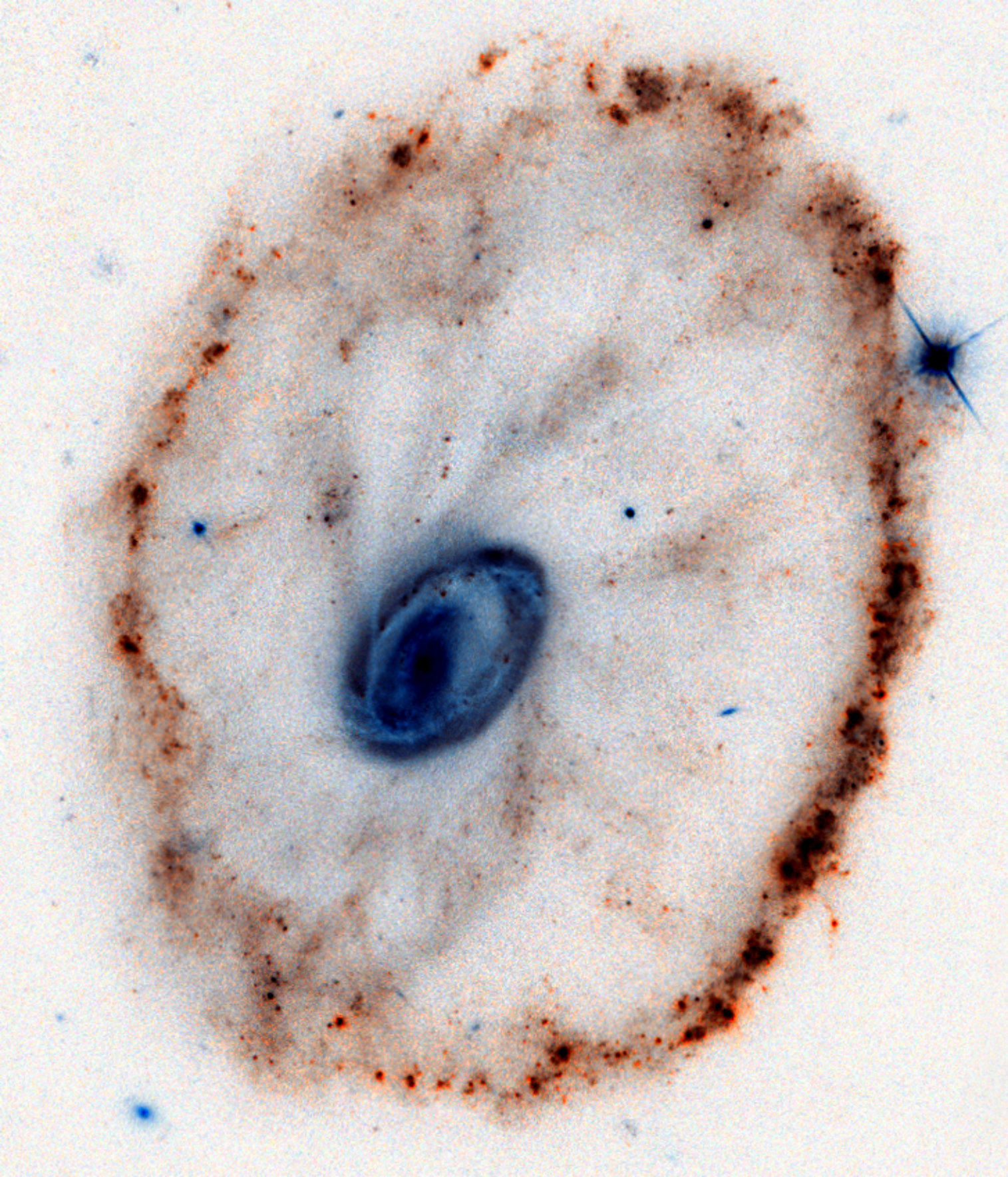 Figure 1
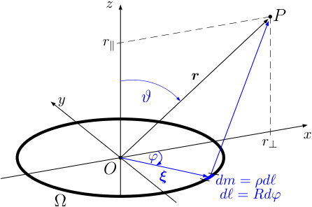 Figure 2
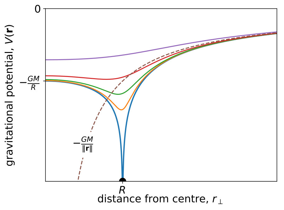 Figure 3
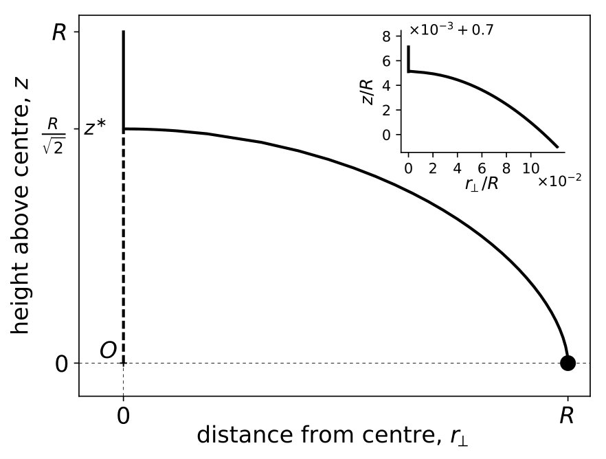 Figure 4
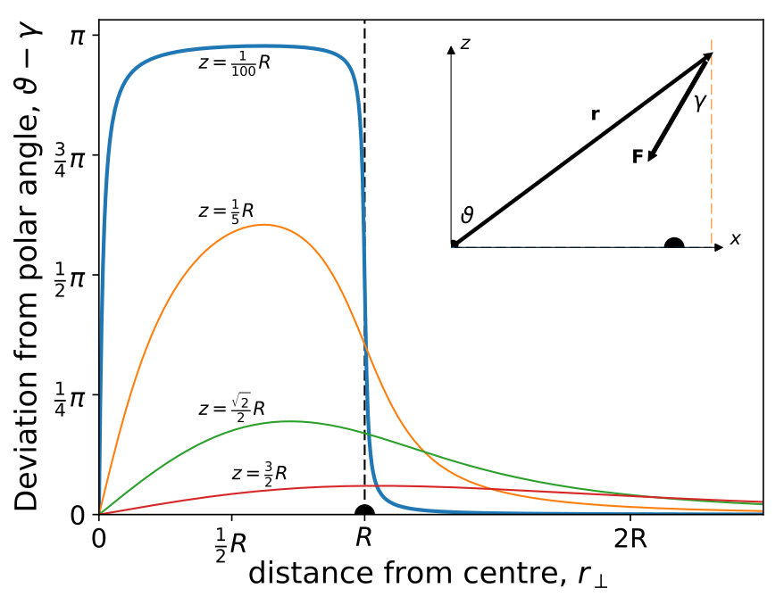 Figure 5
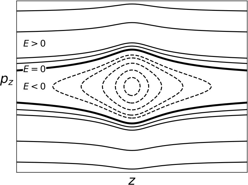 Figure 6
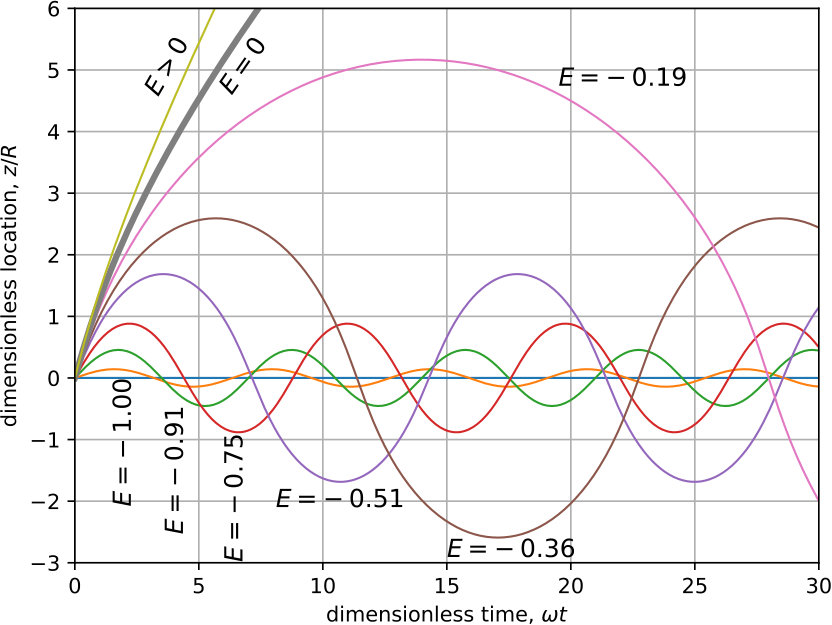 Figure 7
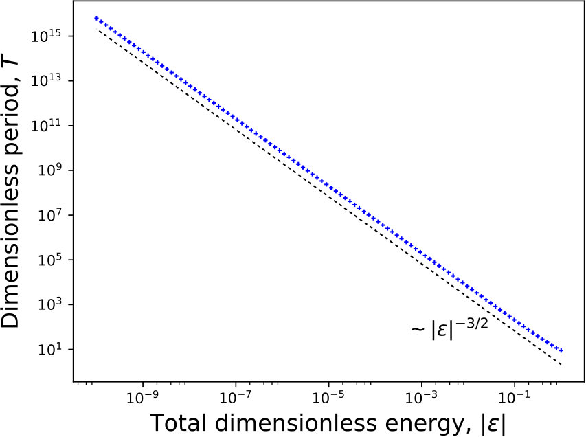 Figure 8
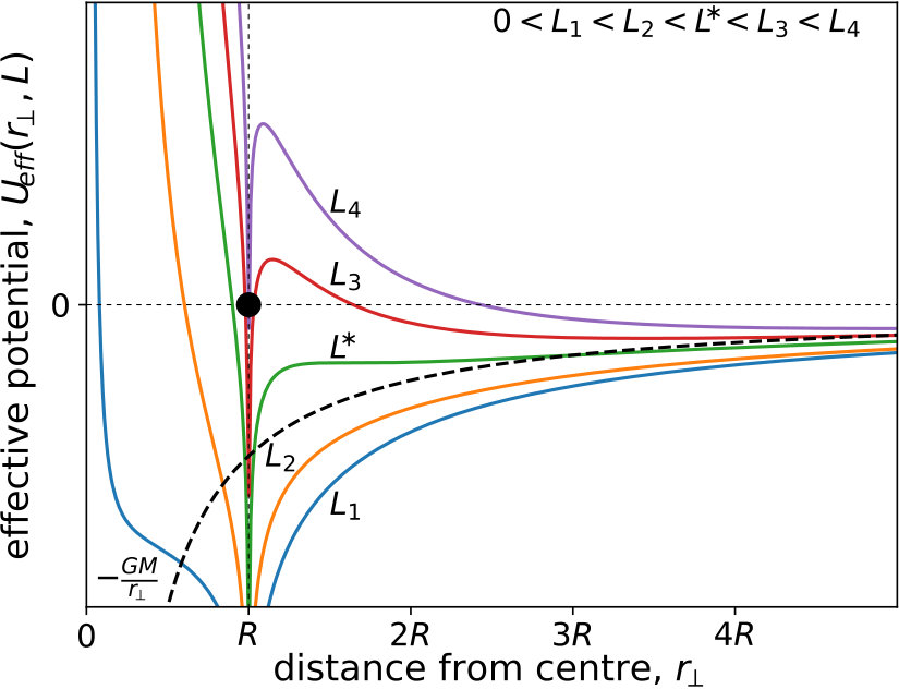 Figure 9
Peer Reviews
No public reviews on file for this paper yet. If you reviewed it on a platform where reviews are public (OpenReview, ICLR, NeurIPS, ICML), you can paste yours below so the community can read it here.
Videos
No videos yet. Explain this paper in a talk, walkthrough, or lecture? Add one.
Peculiarities in the gravitational field of a filamentary ring
Dániel Schumayer
David A. W. Hutchinson
The Dodd-Walls Centre for Photonic and Quantum Technologies, Department of Physics, University of Otago, Dunedin 9106, New Zealand
Abstract
The gravitational field of a massive, filamentary ring is considered. We provide an analytic expression for the gravitational potential and demonstrate that the exact gravitational potential and its gradient, thus the gravitational force-field, is not central. Hence it is a good candidate to discuss the difference between the concepts of center of mass and center of gravity. We focus on other consequences of reduced symmetry, e.g., only the -component of the angular momentum is conserved. However, the remnant high symmetry of this system also ensures that there are special classes of motions which are restricted to invariant subspaces, thus, depending on the initial condition, the dynamics of a point particle is integrable. We also show that periodic orbits in the equatorial plane external to the ring are possible, but only if the angular momentum is above a threshold value. In this case the orbits are stable.
I Introduction
From the earliest evidence regarding the activities of our ancestors, we know that stargazing and attempting to explain celestial events, the motion of Sun, Moon, and, perhaps, constellations were important to everyday life. In cave drawings and rock carvings one can find motifs of archaeo-astronomical significance.Mourão (2009); Norris and Hamacher (2011)
Why all these celestial bodies move the way they appear to move? What forces of nature govern their behaviour? These questions occupied natural philosophers for centuries and, with numerous contributors, they received a quantitative answer in Newton’s Philosophiæ Naturalis Principia Mathematica (Mathematical Principles of Natural Philosophy) in 1687. Apart from giving the foundational rules for classical mechanics, Newton also provided a theory of gravity. His inverse-square law could explain and predict –to a higher accuracy than its contemporary theories– how planets are orbiting in our solar system.
In most undergraduate courses on classical mechanics this Newtonian theory of gravitation is taught, predominantly applied to only point particles and/or spherical objects, such as the Sun and Earth.Jones and Childers (1993); Halliday et al. (2004); Giancoli (2008); Serway and Beichner (2000); Urone et al. (2012); Hewitt (2013); Knight (2013) In the latter case, it is undoubtedly mentioned that one may calculate the gravitational attraction between two spherical objects if their masses were concentrated in their individual centers and one rather calculated the force between these point particles. Furthermore, the same process applies if density of each of these spherical objects varies only with the distance from the center. Planets and stars can be treated as such spherical objects, at least in the leading order. Despite the necessarily simplistic analytic treatment of the dynamics of gravitating bodies in undergraduate entry courses, one can find useful supplementary materialGreen (2015) with numerical simulations which could help students develop a good intuition about motion under the influence of non-central forces.
The idea of replacing an extensive object with an abstract massive point particle is extremely powerful, conceptually simple, and essential to efficient modelling of physical processes. It is also rarely mentioned that for non-spherical objects one may not apply this rule of thumb directly. Seldom are the concepts of “center of mass” and “center of gravity” distinguished. 111In all textbooks cited before all mentions that in uniform gravitational field the center of mass and center of gravity coincide. While this practice is defensible from the view of practicality, we feel that pedagogically is questionable: an exceptional case (point particle or perfectly spherical objects) is taught. Only Ref. Serway and Beichner (2000), among the already cited textbooks, treats non-uniform mass distribution and non-spherical bodies explicitly in a subsection. The former is uniquely determined by the shape and mass distribution of a body, thus it is a well-defined point. However, the center of gravity depends on the interaction of two gravitating bodies, thus it may not be a fixed point as the case of spherical bodies would indicate. The example system examined below demonstrates the inapplicability of this rule of thumb for a very simple system.
Here we study the gravitational potential of a massive, ideal ring and the motion of a massive point particle in this field. The simplicity, finitude and the high degree of symmetry of this geometry motivated our analysis. One might object, saying that an infinite line would truly have even simpler geometry. However, with uniform mass distribution, it would have infinite mass. Also we would like to preserve as much of the spherical symmetry as possible, and the field of a ring has cylindrical symmetry.
There are two other –admittedly less weighty– motivations for this work. First, the orbits of numerous planets can be considered to be ring-like, and during their revolution around the center their own gravitational field perturb the motion of other planets, moons, comets, etc. Gauss averaging theorem states Gauss (1818); Abad and Belizon (1997); Boccaletti and Pucacco (2013) that the secular perturbative effect of a revolving object can be calculated by spreading its mass around its orbit uniformly and determining the perturbation of this ring on the target object. Thus the gravitational field of a uniform ring does indeed have significance in astrophysics.
Second, ring structures have actual importance in galactic dynamics as well. Several celestial objects are more or less spherical, e.g., stars, planets, black holes, but there are other objects, e.g., galaxies, interstellar dust and clouds, whose geometry varies strongly. In our own galaxy, in the Milky Way, there are billions of stars revolving around the center in a thin disk, see Figure 1. The thickness of this imaginary disk is approximately hundred and fifty times smaller than its radius, but a substantial part of the galaxy’s mass is in the disk Zeilik (2002); Carroll and Ostlie (2017). Similarly there are ring galaxies in the Universe, where the millions of stars constituting the galaxy are located along a ring with no or small amount of luminous matter visible in their interiors,Theys and Spiegel (1976, 1977) e.g., Cartwheel Galaxy in Figure 2.
In this work we aim to provide a simple enough system which can be analytically analyzed at the graduate level, but whose gravitational field holds peculiar features, e.g., it produces a non-central force field. We believe the investigation of such system is beneficial for students as in most cases they only see spherically symmetric bodies whose exterior gravitational field can be determined by that of an imaginary point particle. While the analysis presented here is relatively simple, it may stimulate the Reader’s appreciation of the longstanding challenge of calculating the gravitational potential/field of celestial bodies. As an excellent example, we mention the landing of a small robot Philæ on the comet 67P/Churyumov-Gerasimenko traveling at tens of thousands of kilometers per second. That was the first occasion in history that an expedition successfully landed on a comet. The estimation of the gravitational field was crucial to achieve such a landing and later measurements allowed for the determination of the inner structure of that comet.Pätzold et al. (2016) Furthermore we may also point at the resurgent interest in analyzing gravitational fields of extended objects, mainly that of the Earth Hofmeister et al. (2018), due to the commercial interest. There are a handful companies, e.g., SpaceX, RocketLab, Blue Origin, manufacturing and launching rockets and placing satellites in orbits on a regular basis. In order to plan the orbits of these spacecrafts and monitor their trajectories, more and more precise models and planning will be required.
II General formalism in a nutshell
Newton’s law of gravitation states that the force between two massive point particles is proportional to the masses of interacting particles, inversely proportional to the square of their distances and lies in the direction of the line connecting the particles. The proportionality constant is denoted by in the following.
Since the gravitational field is conservative, the force can be deduced from a scalar potential, , satisfying Poisson’s equation with mass distribution, . Often the density is given and one seeks the gravitational potential. One can express the potential knowing the Green’s function of the adjoint boundary value problem. Since the Laplace operator equipped with Cauchy boundary condition at infinity (the potential must vanish infinitely far from the gravitating body) is self-adjoint, the adjoint Green’s function, , coincides with the Green’s function of the original problem, . Thus the Green’s function, , provides the potential
[TABLE]
Although the natural domains of and are identical, the three-dimensional space, we only analyze cases where the density distribution, , is restricted to a domain of finite size, , which is occupied by the fixed mass distribution. For an idealized, filamentary ring denotes the circumference of the ring, while in the case of an annulus and a disk is the surface area of these objects. Since is assumed to vanish completely outside of , the integral on the right hand side of Eq. (1) is also interpreted to be over only .
It is worth recognizing how the potential is affected by scaling the density and distance. If and denote two non-zero numbers, then Eq. (1) shows that scaling the density by a factor of would result in scaling the potential by too, i.e., , and similarly . As a consequence, one could opt for calculating the gravitational potential of a ring of unit mass and unit radius, since the result can be scaled to the actual mass and radius. This scaling property of the potential can be useful when one writes a numerical code, for example, to simulate the motion of an object under the influence of the ring’s gravitational potential. However, for the sake of clarity and being explicit we keep both the mass and the radius of the ring as variables.
Here we mention two recent analyses of the electrostatic potential and electric-field of a charged ring. As the gravitational potential and the electrostatic potential both satisfy Poisson’s equation, the same mathematical machinery can be employed in both cases. However, the dynamics of an external charge heavily depends on whether the interaction is attractive or negative. Zypman considered Zypman (2006) the electric field of a uniformly charged ring and put the emphasis on an intuitive introduction of the potential and visualizing the electric field using a mathematical software package. In connection to our interests here, the sketch of the electric field in the plane implicitly showed that the field, and thus the force on a point charge is not central. Selvaggi *et al. *employed Selvaggi et al. (2007) a different approach and demonstrated –without detailed introduction of the toroidal functions– that the electric potential can be expressed in a compact form using the Fourier cosine expansion of the , in which expansion the toroidal functions appear as coefficients of the functions. This approach has some numerically attractive features: any non-uniform charge distribution can be systematically analyzed after calculating the Fourier expansion of the charge distribution on the ring, and for each term in this expansion there is a single corresponding toroidal function. However, the choice of toroidal functions of first or second kind may require further thoughts. In Selvaggi et al. (2007) only the second kind is used, while in the mathematical literature it is used predominantly for the interior problem, .
III Gravitational potential of a ring
Let us examine an ideal ring whose total mass, , is distributed uniformly along the circumference of a circle of radius , thus . This system is regularly in the focus of classes on classical mechanics and non-relativistic electrodynamics, although the gravitational or electrostatic potential is determined almost always along the symmetry axis, , perpendicular to the plane of the ring.
The plane of the ring divides the three-dimensional space into two halves and the potential will thus have a reflection symmetry with respect to this plane, i.e., . Furthermore, the potential is rotationally invariant along the -axis which crosses the center of the ring and perpendicular to the plane of the ring.
One may determine the gravitational potential at point by carrying out the integration in Eq. (1) along the ring. Due to all symmetries, however, one may fix the Cartesian coordinate system in such a way that has zero coordinate.
The gravitational potential of the ideal ring at point is given
[TABLE]
where we have introduced , which is the distance of point from the furthest point of the ring, and . In the standard nomenclature of the field of elliptic integrals, parameter is called the modulus. Byrd and Friedman (1954); Abramowitz and Stegun (1972)
The integral above cannot be given in elementary functions, and itself defines a new special function, the complete elliptic integral of the first kind,Byrd and Friedman (1954) , with modulus . It is apparent that this integral is real only if , and it is singular only if . One may easily check that remains in the interval for any and it becomes unity only at the points of the ring itself. Consequently the gravitational potential becomes singular only “on” the ring. This is expected and it is due to the inherent nature of Newton’s gravitational law itself. However, the strength of singularity is milder than as anticipated from Newton’s law for point particles. Since for , thus for the denominator of the integrand is . Therefore the integral locally behaves as , i.e., the singularity is logarithmic rather than power-law.
Finally the gravitational potential isLass and Blitzer (1983)
[TABLE]
and it is plotted as a function of for some fixed height values in Figure 4. The singular curve corresponds to the gravitational potential in the plane of the ring, i.e., , while the for other curves, . The potential along the symmetry axis has a value of , in agreement with standard elementary treatment. While Figure 4 clearly shows that the potential indeed becomes shallower at the center for higher value, it is interesting to note that the gradient of for small values is negative, but as increases it turns to positive. In other words, the potential is repulsive at the center of the ring if the height is below some threshold height, , but for heights the center becomes attractive and it is the global minimum of the potential. It is fascinating that in a simple gravitational system the potential changes its qualitative behavior along a symmetry axis not smoothly but abruptly.
We can determine the threshold height at which the potential sways from attractive to repulsive. We have noticed that at fixed the potential develops a minimum at a finite . The location of this minimum, i.e., the can be determined by taking the first derivative of with respect to and equating it to zero. After some straightforward calculation one obtains the equation, which establishes the relationship between and at the minimum:
[TABLE]
where is the complete elliptic integral of the second kind.Byrd and Friedman (1954) Although this equation seems intractable to express in terms of at the minimum or vice versa, let us remember that at the threshold height, , the symmetry axis becomes the global minimum, thus at this height this equation must support a solution of . Furthermore, at the modulus becomes zero, and both complete elliptic integrals are not only finite for such modulus, but . However, we cannot blindly substitute and into the equation above, as it would lead to the trivial identity; the first term vanishes because of the factor , while the second factor is zero due to . Thus we have to determine the solution of Eq. (4) in the limit of . The series expansion of both special functions are well known (see formulas 900.00 and 900.07 in Byrd & Friedman’s monographByrd and Friedman (1954)) and can be readily employed in this equation. After inserting these expansions, truncated at the order, we arrive at
[TABLE]
The is always a solution for any value. However this expression does not say whether that is the minimum or maximum of the potential. From Figure 4 we deduced that for the potential will attain its local maximum at . As we are seeking the location of minima we need to examine the expression in the square brackets, and perhaps express in terms of :
[TABLE]
As we derived this expression in the limit, this result is valid only around the symmetry axis. We can immediately read off , as . Thus . The Reader may verify this result as follows. As Figure 4 indicates the center of the ring is always an extremum of the potential; at the potential has a maximum, while at higher altitude along the -axis become a global minimum of the potential develops. In other words the second derivative of the potential, with respect to , changes sign from positive to negative at the threshold point, . Thus one needs to solve the equation
[TABLE]
for with fixed thus . Although this expression still contains both elliptic integrals,444An even simpler approach would be to first substitute into the expression of the gravitational potential and obtain and then differentiate this expression twice and solve the equation for . their values can be factored out after substituting in, since . One then arrives at the second order equation , which indeed confirms the value of .
Another interesting feature of the gravitational potential in Figure 4 is the appearance of a global minimum provided is kept fixed and , within the ring, . This fact may –incorrectly– suggest that a particle can be in stable equilibrium in the inner vicinity of the ring, away from the center, since no force would be exerted on a particle as vanishes at the minimum. The crux of this fallacy lies in omitting the gradient of the potential in the direction at the minimum, i.e., .
Before we shift our focus to the dynamics in the gravitational field of a ring, let us briefly examine and quantify how much the force field deviates from a central field. The cylindrical symmetry guarantees that neither the potential, nor the force depend on the azimuthal angle, . However, after expressing and (see Eq. (3)) in spherical coordinates
[TABLE]
it becomes apparent that the force does depend on and, as a consequence, it cannot represent a central force. In order to visualize and quantify how much the force deviates from a central field, let us calculate the difference of angles, and the polar angle, (see inset of Figure 6). For radial force these two angles should be either equal in absolute values, thus their difference is either zero or . In Fig. 6 we have plotted their difference, , as a function of for fixed heights, . The graphs show that this difference changes abruptly closer to the plane of the ring, and confirms that for the two domains (inside and outside the ring) behave quite differently, although in both cases the force points towards the ring. Inside the ring , while outside .
As increases the angle difference drops, but still changes significantly, reaches its maximum “inside” the ring, and diminishes rapidly as . However, as increases further the angle difference vanishes and the maximum becomes very wide.
IV Dynamics in the gravitational field of a ring
In classical mechanics one often examines the dynamics of a particle under the influence of a central force; the force can be written as , i.e., the magnitude of the force, , and its direction, , are decoupled and the direction is always parallel to . Since physically important forces, e.g., gravitational attraction and electrostatic interaction, fall into this category the analysis of this special type of forces is warranted. It is proven that the trajectory of a particle moving in a central force field lies in a plane, and the angular momentum of the particle, , is a conserved quantity. If, furthermore, depends only on , then the force field is conservative as well, thus total mechanical energy is conserved along any trajectory. This special case is the one which is often analyzed in university courses.
However, even the gravitational attraction of an ideal ring is more complicated than this special central, conservative force field. While is cylindrically symmetric, it is not spherically symmetric, ergo depends on the distance from the center, , and on the polar angle, , too. There are only two special sets of trajectories along which a particle would experience a central, conservative force field: (a) along the -axis, and (b) on any trajectory lying in the -plane of the ring. Therefore in these two cases we can invoke energy and angular momentum conservation, and thereby reduce the degrees of freedom to one. Since these two sets are also part of the invariant subspaces of the potential, a particle remains in these subspaces provided its initial momentum is also parallel to these subspaces: in case (a) and (b) . In case (a) this constraint also means that the angular momentum vanishes identically.
For later use it seems worthwhile to record the expression of force at an arbitrary point in space. For sake of transparency the force is rescaled by a unit , and also the coordinates are given in units of . Due to rotational symmetry around the -axis, the force at any point should lie in the plane which includes and the entire -axis, i.e., the force depends only on the distance of from the -axis and from the equatorial plane. Therefore the force can be expressed as
[TABLE]
where is the interaction potential between the ring and the massive particle orbiting in the field of the ring. After some relatively straightforward calculation we can express the force in the form:
[TABLE]
with the dimensionless factor
[TABLE]
In general, the component of the total angular momentum, , along an axis about which the field is symmetrical is always conserved,Landau and Lifshitz (1982) thus is conserved. Based on the results shown above we can easily check for this by calculating the Poisson-bracket of and
[TABLE]
where and analogously . This Poisson-bracket involves the partial derivatives with respect to the coordinates and the conjugate momenta. Since the Hamiltonian of a massive particle moving in the gravitational potential of a ring has the traditional form , i.e., the coordinates and the momenta are separated, the derivatives of are simple: while . The derivatives of are also easy to calculate from , hence
[TABLE]
Furthermore, cylindrical symmetry or, in other words, the conservation of , allows one to reduce the number of degrees of freedom of the generic Hamiltonian from three (, , and ) to two ( and ) and obtain
[TABLE]
IV.1 Motion along the axis
Let us first analyze the motion along the -axis. The gravitational potential in Eq. (3) simplifies significantly, as renders to be zero too, thus the elliptic integral, , is only a constant in this expression. The potential is then
[TABLE]
as expected. Because of this reduced effective dimensionality, we can easily create a contour plot, see Figure 7, of the total mechanical energy
[TABLE]
over the phase space. The energy level curves , where partition the phase space into three, qualitatively different types of orbits. In Figure 7 the dashed lines correspond to total energy being negative, , and these trajectories are closed, i.e., in these cases the motion of the particle is periodic. The separatrix, , the curve separating the bounded and unbounded trajectories, is emphasized in the same figure with thick solid line. While this motion is not limited in coordinate space, the particle reaches , however, its speed is zero at infinity. Trajectories with positive total energy are also unbounded, but the particle reaches infinity with a finite velocity.
Here we mention that this Hamiltonian –after re-scaling– coincides with that of for the century-old MacMillan problem,MacMillan (1911) a special three-body problem.
In Figure 8 we plot the instantaneous deflection, , of a particle moving along the axis. The corresponding total energy is also given for all paths. As one expects, for lower, negative energies, the amplitude is small and the motion resembles harmonic motion. However with increasing energies the curve deviates from a sinusoidal undulation as a function of time and its shape morphs into more of half-circles, see for example , and the period increases rapidly. At the function loses its periodicity. In the – graph this path separates the periodic paths from the diverging paths.
It is worth investigating how the period depends on or varies with the total energy. After a significant amount of algebraic manipulations one may express the period of the closed orbits as
[TABLE]
where , the modulus , and parameter is the dimensionless energy of the moving particle. The integral cannot be expressed in terms of elementary functions, however, its structure suggests that a closed form can be given in terms of complete elliptic integrals. We omit analysing this closed form, as the main characteristic features of the period can be deduced from the integrand directly555For the sake of completeness we provide here the exact expression for the period
T=\frac{4}{\omega}\,\frac{1}{2(1-2k^{2})}\,\Bigl{[}2E(k^{2})-K(k^{2})+\Pi(2k^{2}|k^{2})\Bigr{]}
in terms of the complete elliptic integrals of the first, second and third kind, , , and , respectively. Their definitions can be found in Byrd and Friedman (1954). The power series expansion of this exact expression, up to second order, agrees with that of given in the text, , but derived from a hand-waving argument..
First, the integrand has a singularity at , due to the term, irrespective of the value of . However, this singularity on its own is quite mild and, provided , the other two terms remain finite and the integrand remains integrable.
Second, small amplitude motion along the axis around the center of the ring corresponds to , thus , and can be thought of as a harmonic oscillation around the center. For small values one may expand the integrand in Taylor series, and integrate term-by-term
[TABLE]
The leading order is the classical result, . This result also gives the first correction as the energy increases. Although further terms of the Taylor expansion have been omitted, it seems reasonable that all these terms contain even powers of , thus all terms will be positive as energy increases towards zero.
Third, as the energy approaches zero, or alternatively as , two terms become singular at in the integrand of Eq. (15). In the following we examine the behavior of the integrand for , where . The third term, is not singular, it remains finite for all possible and values, thus we omit it as it can be thought of a weight-function. Keeping this term would not change the -dependence of the period, but would only contribute a constant pre-factor. The remaining integrand suggest a change of variable, , where runs over . In this new variable the integration can be carried out analytically if .
[TABLE]
Figure 9 depicts the period, as a function of the absolute value of the dimensionless energy, . The derivation above suggested a power-law dependence, thus a log-log scale plot is chosen with the absolute value of the energy as abscissa. Therefore, paths with lower energy are towards the right of the plot, while the period of trajectories with energy close to zero are towards the left of the abscissa. The blue crosses represent the numerical values of periods as calculated from Eq. 15 via quadrature, while the thin dashed line represent the power-law, , derived from our approximation. The two “curves” seem to be parallel, indicating that there is a constant multiplicative factor missing from our approximating power-law. This is indeed the result of us completely neglecting one, non-singular term in the integrand. Although we may have expected this approximation to be valid only as , it proves to be a surprisingly good approximation in the entire interval examined. One might think that for even lower energies the deviation between the numerical values and the power-law would increase, as the slight curve appears in the blue crosses towards , however, we should keep in mind that the energy of a particle moving along the axis cannot be arbitrarily small, because the gravitational potential energy has a local maxima at , namely as seen in Fig. 4. Since the kinetic energy is always a non-negative quantity the minimal value of the total energy, , corresponds to the minimal value of the gravitational potential along the axis, i.e., . Thus .
IV.2 Motion in the -plane
If a particle is initially located in the equatorial plane of the ring and its initial velocity also falls into this plane then the entire trajectory of the particle will remain in the plane. Furthermore, the cylindrical symmetry guarantees that the force at any point points towards the origin, thus the motion in this plane is a central force problem. Consequently there is a supplementary conserved quantity on top of total mechanical energy, namely, the angular momentum, with magnitude .
A particle does have two degrees of freedom moving within a plane. However, the conserved quantities help us reducing the number of equations of motion to one (see §14 in Landau and Lifshitz (1982))
[TABLE]
The first term can be written as a derivative with respect to , thus one might combine these two terms and interpret the equation of motion so that the particle is under the influence of the effective potential
[TABLE]
Figure 10 shows the effective potential for four values of and unit mass, . There are several features of the graphs which are worth some analysis. First, the singularity at is due to the inherent singularity of the gravitational potential itself and it is not the consequence of the specific geometry. Second, irrespectively of angular momentum the effective potential is strictly decreasing for . This behavior gives further support to the fact that there cannot be a stable trajectory “inside” the ring; for increasing angular momentum the effective potential is stepper and steeper towards the ring. Even the case, i.e., the motion parallel to the -axis, is not an exception. It is unstable against perturbations, since the effective potential develops a local maximum for and and not a minimum. Third, in the case of , one may see that for a yet undetermined, threshold value , a shallow but wide minimum develops in the effective potential. This feature indicates that stable, periodic orbits may exist further away from the ring.
Thus a particle with the corresponding energy and appropriately chosen initial location can be in a stable, dynamical equilibrium in real space. For further increasing the angular momentum (subfigure (c)) the potential well grows in size (more and more closed lines appear in the plot) and also moves away from ring as expected.
It seems worthwhile to find out the critical angular momentum, , at which the dip appears in the effective potential.
In order to capture this peculiar behavior, i.e., the appearance of a critical angular momentum value, we may calculate the derivative of the effective potential in Eq. (16), with respect to and equate it with zero. Doing so and expressing we arrive at
[TABLE]
where , with , is the square of the dimensionless angular momentum, and is the dimensionless distance in -plane. Naturally the left-hand-side of this equation needs to be non-negative, therefore this equation has physical relevance only for those values for which the right-hand-side is also non-negative, and then this equation provides the pair (, ), or equivalently (, ), for which the effective potential has local extremum.
The right-hand-side of Eq. (17) is plotted as a function of (the modulus, , is also a function of ). Inside the ring () there is no physical solution, as is negative. Consequently there is no path inside the ring which could be stable; a moving particle is attracted to the ring and inevitably collides with it. However, outside of the ring, we observe that there is either no physical solution, or there are two. The curve defines a minimal distance , and minimal angular momentum, , at which a local minimum starts developing in the effective potential. We need to distinguish two segments of the curve in the region depending on the relative values of and . The interval corresponds to the local maximum of the effective potential (see Figure 10) and thus represents unstable orbits. However, the pairs in the domain all correspond to the local minimum of the effective potential and define stable orbits in the gravitational field of the ring provided the motion is confined to the plane.
The Taylor expansion of the complete elliptic functions, and , around would also provide the asymptotic behavior of the curve in Fig. 12, i.e., . Here, we recovered the classical result for circular orbits around a point-like attractive center, i.e., , where is the distance from the center. Using the unit of again, the dimensionless square of the classical angular momentum is . Figure 12 shows this classical result as dashed blue line and it is the asymptote for as .
Finally we demonstrate that stable and periodic, circular orbits do exist in the equatorial plane of the ring. Furthermore, our numerical experiments indicate that these orbits are stable not only against in-plane perturbations but against out-of-plane perturbations as well. In calculating the trajectory of a point particle we rely on the explicit expression of the gravitational force given in equation (8).
Figures 13 and 14 show trajectories of particles in the gravitational field of a massive ring. The initial conditions were chosen so that the path is periodic (Fig. 13c), slightly perturbed in-plane (Fig. 13d) or perturbed both in-plane and out-of plane (Fig. 14).
Subplot (c) shows the ring (black inner circle) and the orbit (blue circle) in the -plane, with the black triangle indicating the initial location, . The initial velocity is entirely in the direction and its magnitude is chosen so that a circular path is formed. The time evolution of the particle’s distance from the center, is shown above, in subplot (a) as a function of time. It is apparent that it does not change more than the numerical floating-point precision. The orbit on the right, in subplot (d), is started as in (c) but its initial velocity is perturbed in the direction. It is clearly visible in Fig. 13(d) that the orbit does not close any more, but it forms a rosetta, confined between two concentric circles. The stability –at least against perturbation within the equatorial plane– is indicated by subplot (b) depicting a seemingly periodic variation of around the exact circular path with radius . It is easily interpreted based on the effective potential in Fig 10. As the effective potential develops a dip in the region a slight perturbation should drive the particle into an oscillation around the dip. As the effective potential is asymmetric around the minimum, see Fig. 11, the oscillation around the minimum is anharmonic. That is indeed what we observe in Fig. 13(b). The black dashed line is a sinusoidal fit to the very first half-cycle. As time progresses the fitted sinusoidal variation and the actual oscillation deviate from each other, demonstrating an anharmonic oscillation. Similar motion is present in astronomical systems, when the relative distance between two objects, e.g., planet and its moon, varies slightly with time.
Similar calculations can be made by modifying the perturbing velocity component, for example in the -direction as well. Here, without detailed analysis, we include only one figure, Figure 14, showing the trajectory of a particle (blue line) in the gravitational field of a massive ring (black circle). The particle is released with nearly identical initial conditions as in Fig. 13(d), but a small velocity component in the -direction was also added to its initial velocity. The projections of its trajectory is also shown in all three planes drawn with red lines. The projection is similar to that of in Fig. 13(d), i.e., the path remains between two concentric circles, while the other two projections confirm that the path remains within well-defined limits (boxes). In other words, the inhabitants of Ringworld could also invest in launching satellites which are whizzing around their peculiar planet and provide the Ringlings with GPS. The general relativistic calculation for the temporal shift to their clocks is, however, beyond the scope of this article.
Finally we mention that the non-central gravitational field allows unusual, periodic orbits which are absent in central symmetric fields. It is a well-known and often taught result of classical mechanics (Bertrand’s problem) that central force fields in which all bounded paths are closed are that of the harmonic oscillator () and of the spherically symmetric gravitational attraction (), where is a positive constant.Bertrand (1873); Goldstein and Poole (1980); Arnold et al. (1989); Grandati et al. (2008) The non-central field of a massive ring analyzed in this work, provides a relatively simple case where one can construct periodic bounded orbits, e.g., in the shape of in a meridional plane, where the crossing of coincides with the center of the ring. In this work, however, we wanted to focus on the geometric structure of the field, the constraints, e.g., what physical quantity is conserved, and have only touched on the analysis of the dynamics of a point particle in this field.
V Conclusion
In this paper we have analyzed the gravitational field of a massive, filamentary ring and investigated some of the possible orbits of a point-like, massive particle moving in the field of that ring. The choice of a ring was motivated by the high symmetry of this configuration; it possesses continuous rotational symmetry around the axis, reflection with respect to the plane of the ring.
We provided an analytic, closed-form expression for the gravitational potential. One might approach this problem by comprising the entire mass of the ring into its geometric center, and thus calculate at any point in space what potential this point-like object created. However, we demonstrated that the exact gravitational potential and its gradient, thus the gravitational force-field, is not central. Depending on the location of the “test mass” the gravitational attraction exerted on it points at different locations.
Another consequence of the reduced symmetry, or in other words, the non-central force-field is that the angular momentum, in general, is not conserved. However, the continuous rotational symmetry around the fixed axis guarantees that the component of the angular momentum, , is indeed a conserved quantity irrespectively of the motion. Furthermore the high symmetry of this system also ensures that there are special classes of motions which are restricted to invariant subspaces, i.e., motion along the -axis, motion in the equatorial -plane or motion within any meridional plane. This means that the trajectory of a particle remains in a plane if its initial velocity also parallel to this plane. In this special cases the motion is integrable, as the particle has only one-degree of freedom.
We have also shown by analyzing the equatorial motion that inside the ring all trajectories are unstable and eventually the particle collides with the ring. However, outside of the ring periodic orbits are possible, but only if the angular momentum is above a threshold value, . In that case the circular orbit is stable against small perturbations, even if the perturbation is out of plane in contrast to what might naively be expected from symmetry.
Solving the equations of motion numerically revealed that peculiar, and periodic orbits with a shape resembling exist in the meridional planes. Such orbits would not be present in a central force-field, since they would inevitably lead to a collision with the central object.
A more detailed investigation of the dynamics of a point particle in the field of a ring would be warranted as it seems to contain unusual orbits. Furthermore this system –due to its high symmetry– seems to be a great candidate for analyzing the integrability of the dynamics.
Acknowledgements.
D. S. acknowledges the financial support from The Dodd–Walls Centre for Photonic and Quantum Technologies.
The reference list from the paper itself. Each links out to its DOI / PubMed record.
- 1Mourão (2009) R. R. D. Mourão, in Cosmology Across Cultures , Astronomical Society of the Pacific Conference Series, 409 , edited by J. Rubiño-Martín, J. Belmonte, F. Prada, and A. Alberdi (2009) p. 297.
- 2Norris and Hamacher (2011) R. P. Norris and D. W. Hamacher, “Astronomical Symbolism in Australian Aboriginal Rock Art,” Rock Art Research 28 , 99 (2011).
- 3Jones and Childers (1993) E. Jones and R. Childers, Contemporary College Physics (Addison-Wesley, 1993).
- 4Halliday et al. (2004) D. Halliday, R. Resnick, and J. Walker, Fundamentals of Physics , Wiley international edition (Wiley, 2004).
- 5Giancoli (2008) D. Giancoli, Physics for Scientists and Engineers with Modern Physics (Pearson Education, 2008).
- 6Serway and Beichner (2000) R. Serway and R. Beichner, Physics for Scientists and Engineers , Available Titles Cengage NOW Series (Saunders College Publishing, 2000).
- 7Urone et al. (2012) P. Urone, R. Hinrichs, K. Dirks, and R. University, College Physics (Open Stax College, Rice University, 2012).
- 8Hewitt (2013) P. G. Hewitt, Conceptual Physics Fundamentals: Pearson New International Edition , Pearson custom library (Pearson Education, Limited, 2013).