Contextual Predictions for Parker Solar Probe II: Turbulence Properties and Taylor Hypothesis
Rohit Chhiber, Arcadi V. Usmanov, William H. Matthaeus, Tulasi N., Parashar, and Melvyn L. Goldstein

TL;DR
This paper uses global MHD simulations to predict turbulence properties along the Parker Solar Probe trajectory and assesses the validity of the Taylor hypothesis in these conditions, aiding future data interpretation.
Contribution
It introduces a method to evaluate turbulence conditions and the Taylor hypothesis validity using self-consistent MHD simulations for PSP's upcoming orbits.
Findings
Simulations predict large variations in turbulence properties near the Sun.
The approach helps anticipate conditions for better data analysis.
Assessment of Taylor hypothesis accuracy along PSP trajectory.
Abstract
The Parker Solar Probe (PSP) primary mission extends seven years and consists of 24 orbits of the Sun with descending perihelia culminating in a closest approach of (). In the course of these orbits PSP will pass through widely varying conditions, including anticipated large variations of turbulence properties such as energy density, correlation scales and cross helicities. Here we employ global magnetohydrodynamics simulations with self-consistent turbulence transport and heating \citep{usmanov2018} to preview likely conditions that will be encountered by PSP, by assuming suitable boundary conditions at the coronal base. The code evolves large-scale parameters -- such as velocity, magnetic field, and temperature -- as well as turbulent energy density, cross helicity, and correlation scale. These computed quantities provide the basis for evaluating additional useful…
Click any figure to enlarge with its caption.
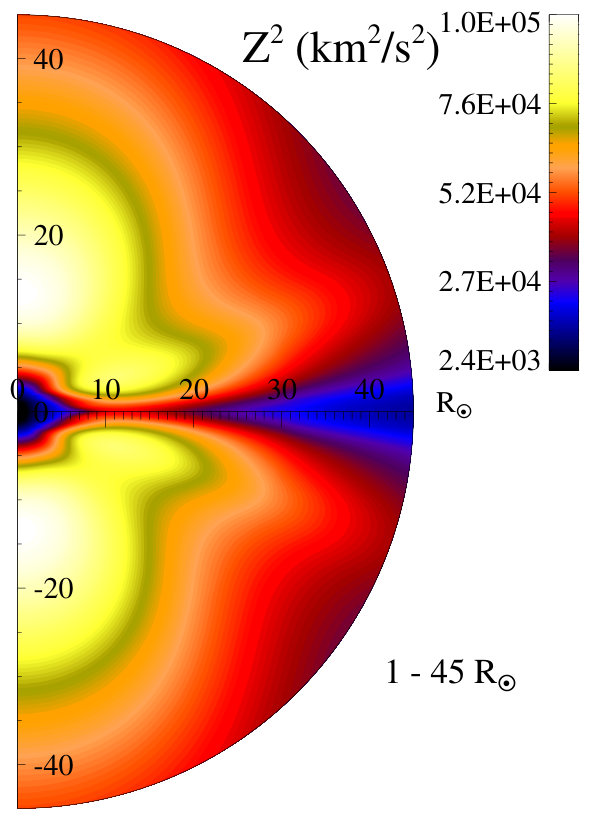 Figure 1
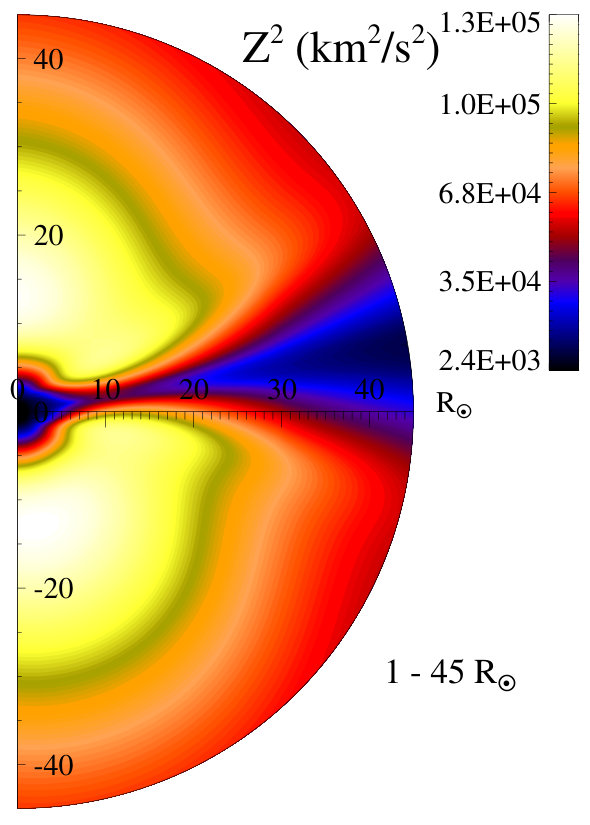 Figure 2
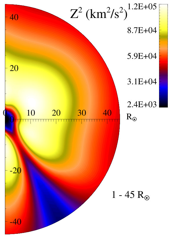 Figure 3
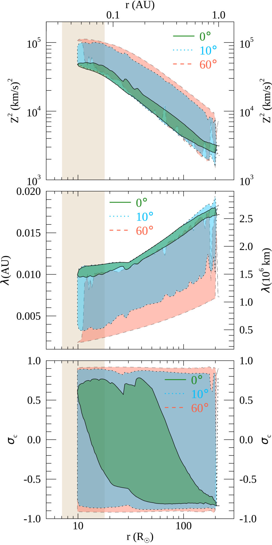 Figure 4
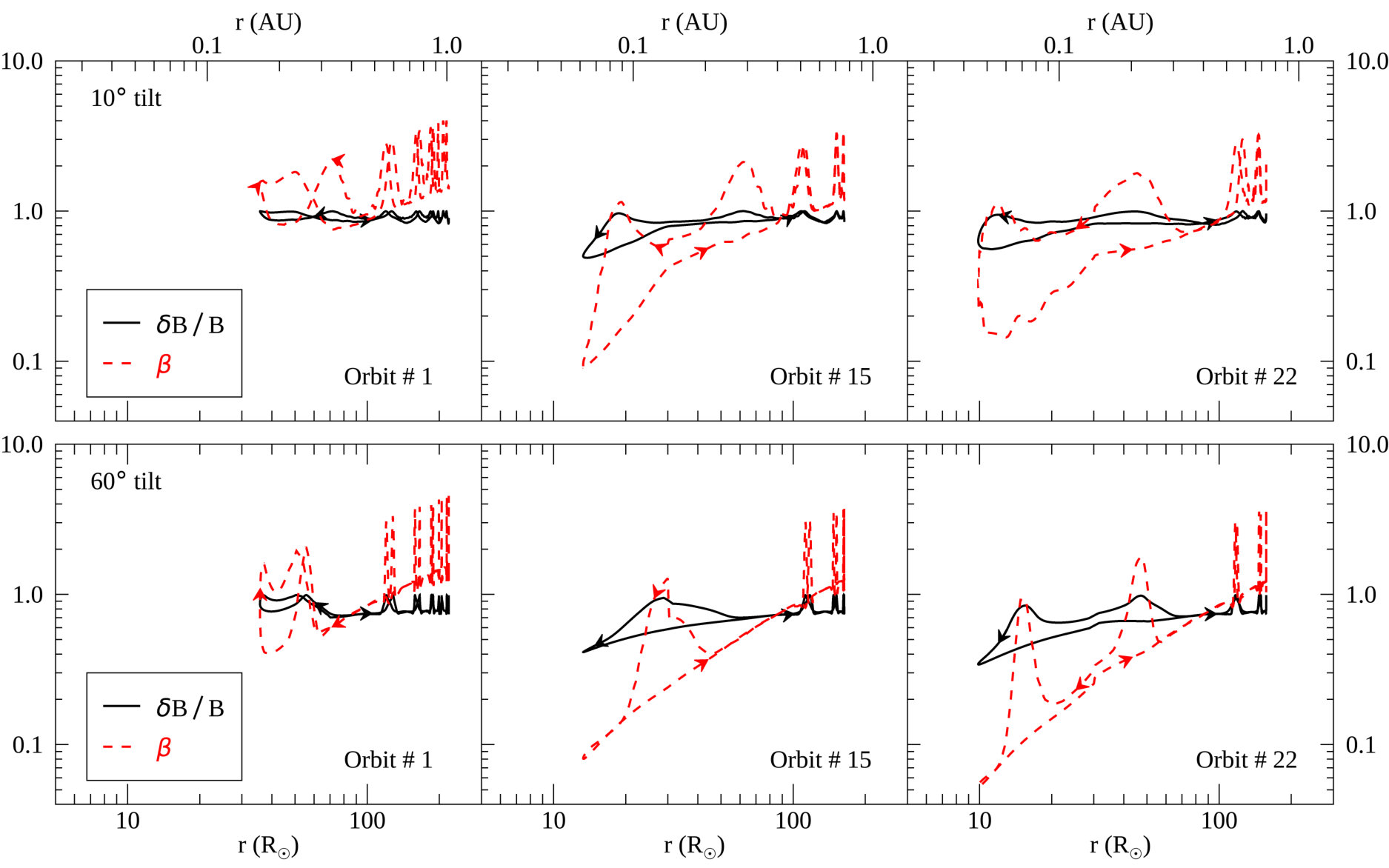 Figure 5
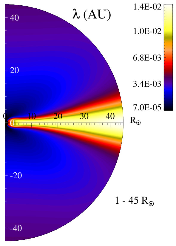 Figure 6
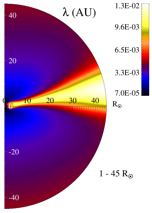 Figure 7
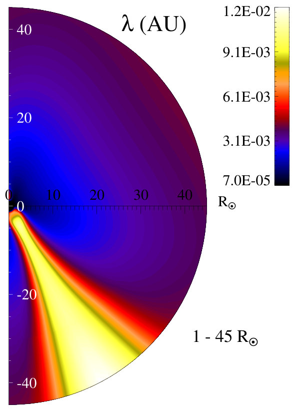 Figure 8
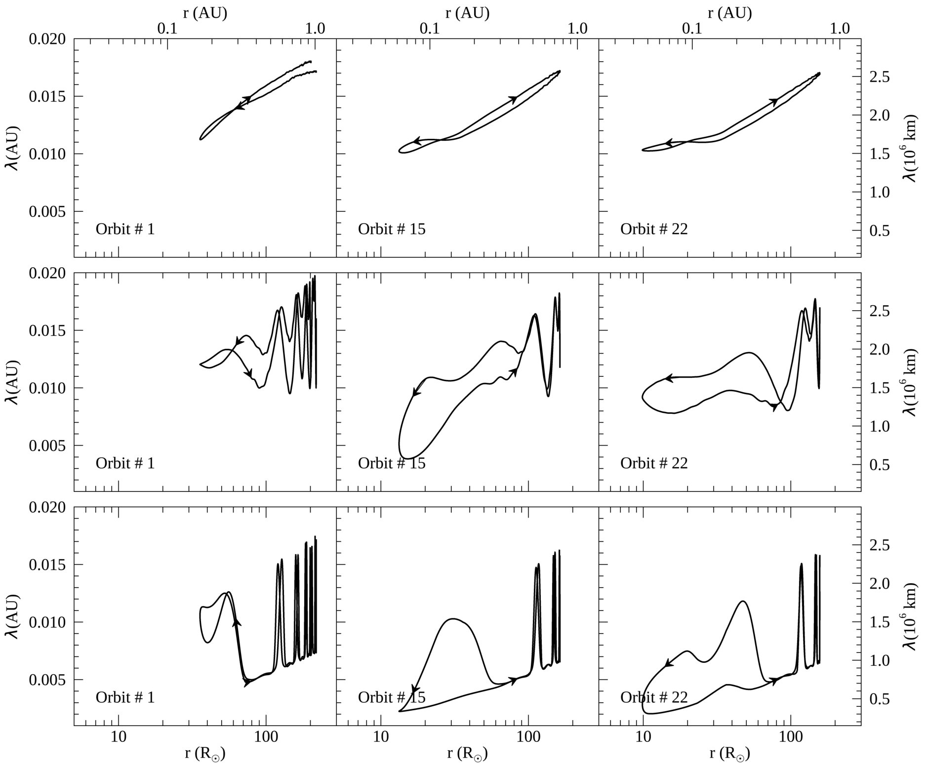 Figure 9
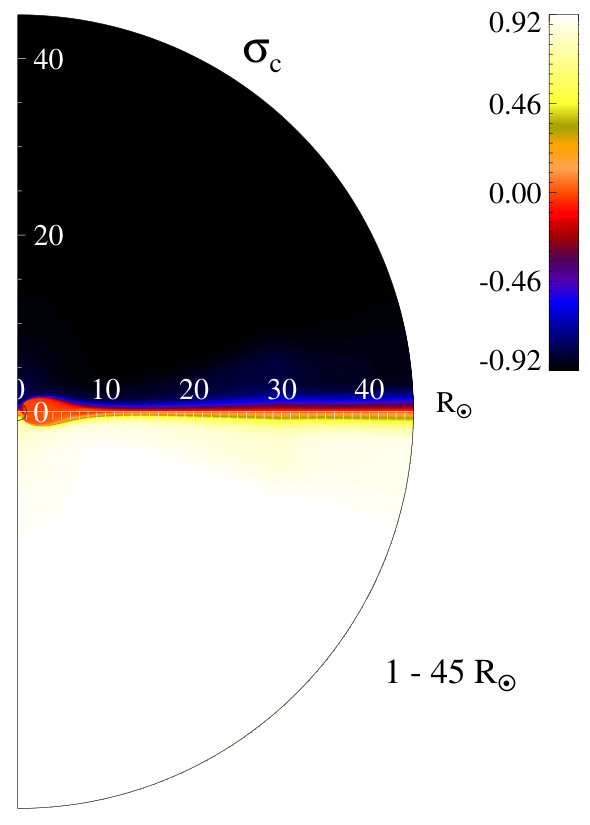 Figure 10
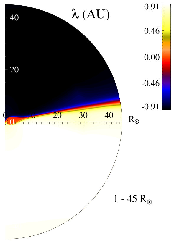 Figure 11
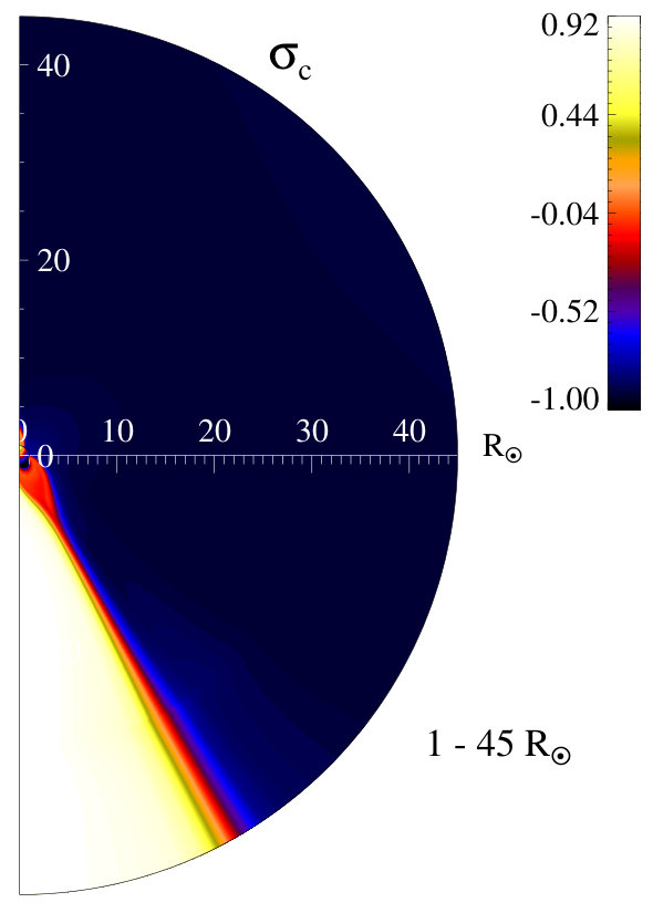 Figure 12
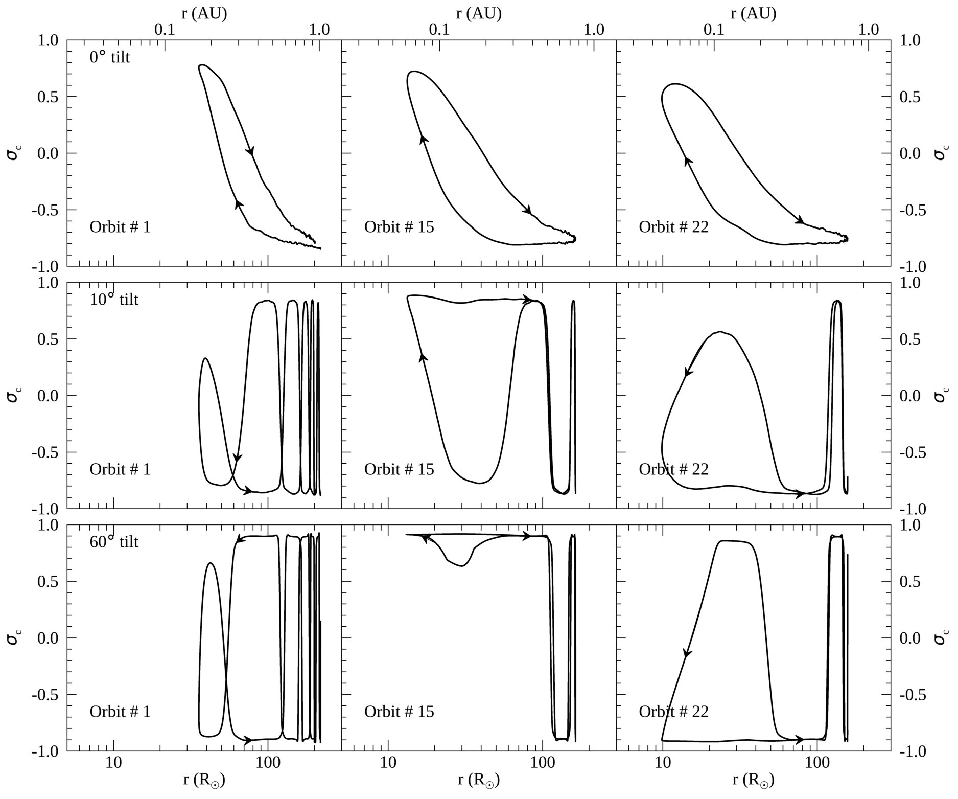 Figure 13
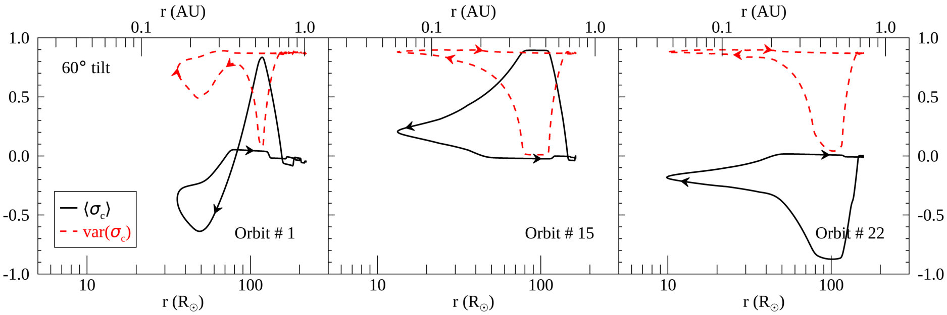 Figure 14
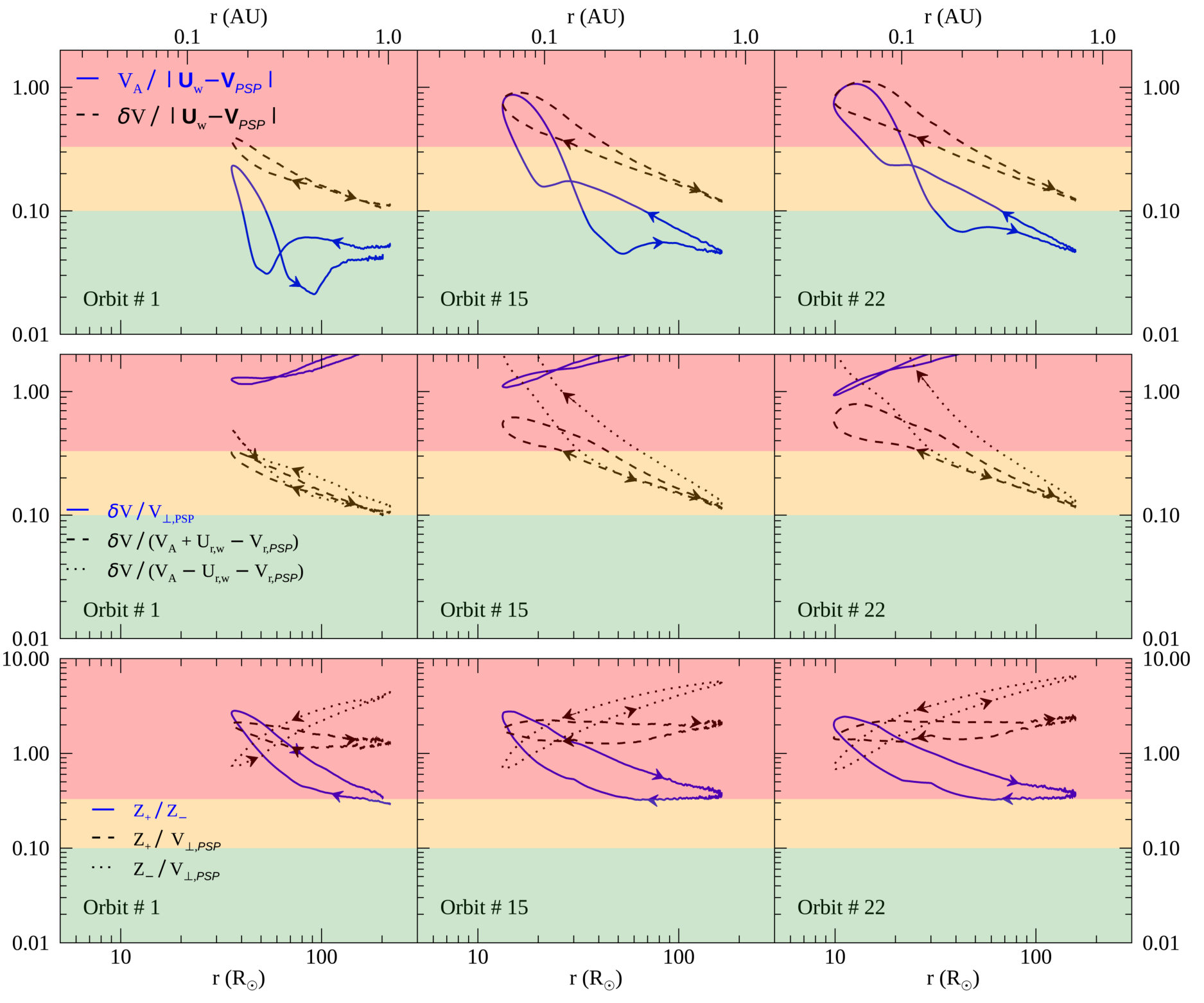 Figure 15
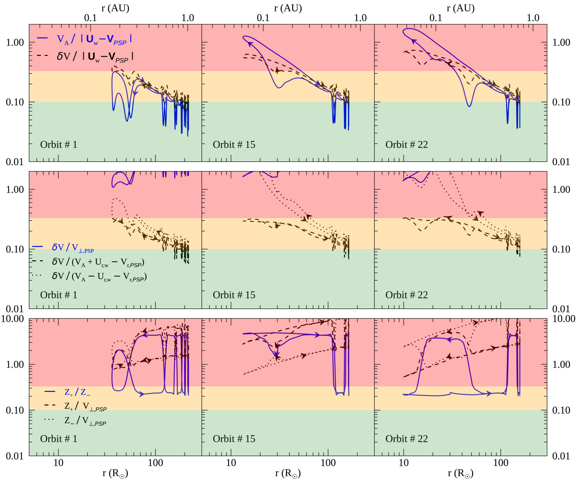 Figure 16
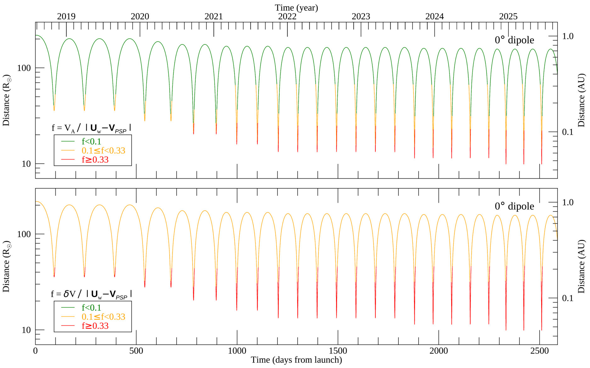 Figure 17
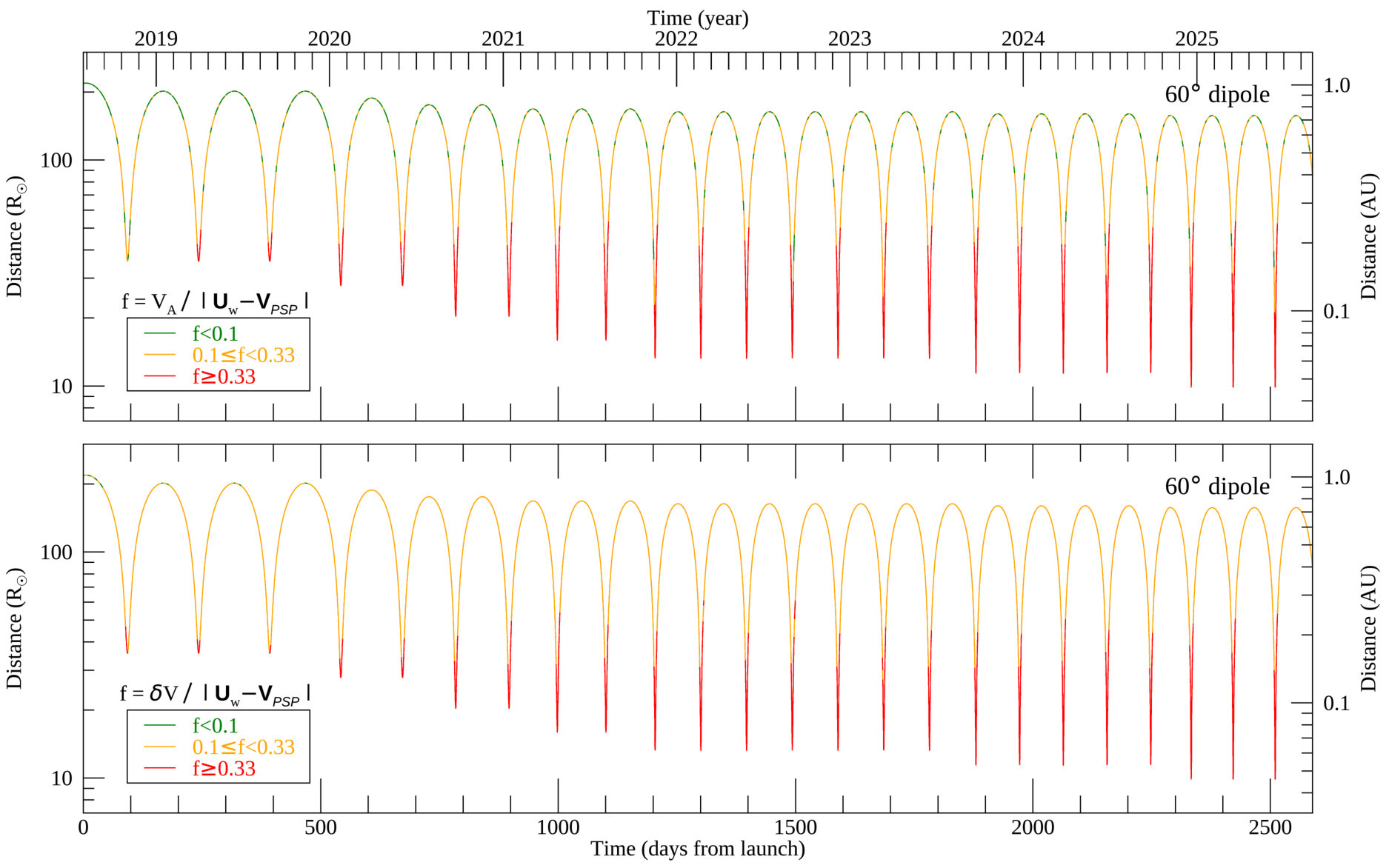 Figure 18
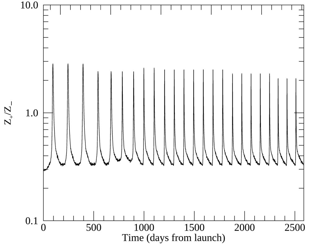 Figure 19
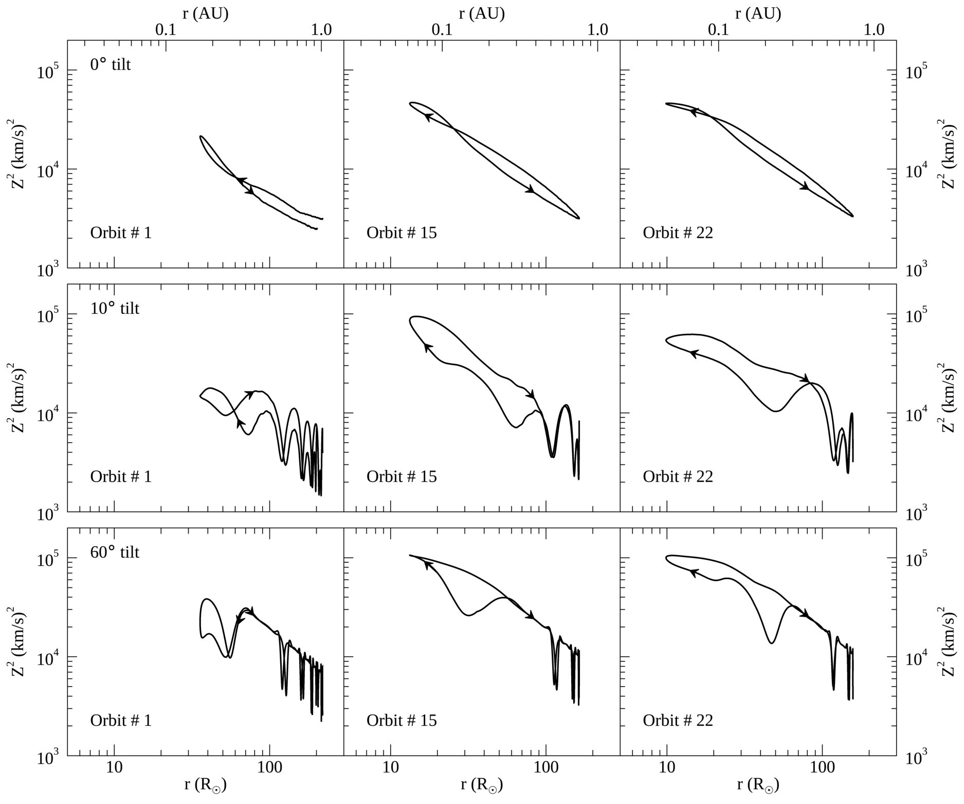 Figure 20
Peer Reviews
No public reviews on file for this paper yet. If you reviewed it on a platform where reviews are public (OpenReview, ICLR, NeurIPS, ICML), you can paste yours below so the community can read it here.
Videos
No videos yet. Explain this paper in a talk, walkthrough, or lecture? Add one.
Contextual Predictions for Parker Solar Probe II: Turbulence Properties and Taylor Hypothesis
Rohit Chhiber
Department of Physics and Astronomy, University of Delaware, Newark, DE 19716, USA
Arcadi V. Usmanov
Department of Physics and Astronomy, University of Delaware, Newark, DE 19716, USA
NASA Goddard Space Flight Center, Greenbelt, MD 20771, USA
William H. Matthaeus
Department of Physics and Astronomy, University of Delaware, Newark, DE 19716, USA
Bartol Research Institute, University of Delaware, Newark, DE 19716, USA
Tulasi N. Parashar
Department of Physics and Astronomy, University of Delaware, Newark, DE 19716, USA
Melvyn L. Goldstein
NASA Goddard Space Flight Center, Greenbelt, MD 20771, USA
University of Maryland Baltimore County, Baltimore, MD 21250, USA
Abstract
The Parker Solar Probe (PSP) primary mission extends seven years and consists of 24 orbits of the Sun with descending perihelia culminating in a closest approach of . In the course of these orbits PSP will pass through widely varying conditions, including anticipated large variations of turbulence properties such as energy density, correlation scales and cross helicities. Here we employ global magnetohydrodynamics simulations with self-consistent turbulence transport and heating (Usmanov et al., 2018) to preview likely conditions that will be encountered by PSP, by assuming suitable boundary conditions at the coronal base. The code evolves large-scale parameters – such as velocity, magnetic field, and temperature – as well as turbulent energy density, cross helicity, and correlation scale. These computed quantities provide the basis for evaluating additional useful parameters that are derivable from the primary model outputs. Here we illustrate one such possibility in which computed turbulence and large-scale parameters are used to evaluate the accuracy of the Taylor “frozen-in” hypothesis along the PSP trajectory. Apart from the immediate purpose of anticipating turbulence conditions that PSP will encounter, as experience is gained in comparisons of observations with simulated data, this approach will be increasingly useful for planning and interpretation of subsequent observations.
Solar wind — magnetohydrodynamics (MHD) — Turbulence — numerical simulation
1 Introduction and Background
Fundamental questions in heliospheric physics concern the heating of the solar corona, acceleration of the solar wind, and the origin of suprathermal energetic particles. At present these questions are actively debated, as we anticipate substantial closure based on the upcoming pioneering observations to be made by the Parker Solar Probe (PSP) and Solar Orbiter (SO) missions. PSP will explore closest to the Sun, within 9 of the surface, and is expected to penetrate the sub-Alfvénic magnetically-dominated coronal region (Fox et al., 2016; Chhiber et al., 2019). These landmark missions will study properties of the interplanetary and coronal plasmas in previously unexplored regions, providing information crucial to understanding structure and dynamics of these plasmas over a wide range of spatial scales. Among the several types of novel measurements to be made by PSP will be measurement of the mean and fluctuating component of plasma density, plasma velocity, and electromagnetic field. These basic measurements will comprise a comprehensive characterization of plasma turbulence at scales ranging from larger magnetohydrodynamic (MHD) scales to subproton kinetic scales. This turbulence provides several ingredients that are potentially crucial in interplanetary dynamics (Matthaeus & Velli, 2011; Bruno & Carbone, 2013). The turbulent cascade of energy is expected to fuel coronal and solar wind heating, and therefore power the distributed acceleration of the solar wind (Matthaeus et al., 1999; Verdini et al., 2010), in addition to direct acceleration by the ponderomotive force of turbulent pressure gradients (Belcher, 1971; Alazraki & Couturier, 1971). Likewise, turbulence provides scattering centers that control spatial transport and diffusion of suprathermal particles such as solar energetic particles (SEPs) as well more energetic galactic cosmic rays (Jokipii, 1966; Chhiber et al., 2017). Turbulence may also play an important role in the acceleration and transport of suprathermal particle populations (Jokipii, 1966; Tessein et al., 2013) and can mediate fast, plasmoid-induced magnetic reconnection (Matthaeus & Lamkin, 1986).
In this paper we focus in particular on the PSP and anticipate measurements of turbulence that it is likely to make. To quantify the turbulence properties – energy density, cross helicity, and correlation scale – we employ a two-scale strategy that is based on a global three-dimensional (3D) MHD simulation model (Usmanov et al., 2014, 2018). This model computes large-scale “resolved” MHD variables – plasma density, velocity, magnetic field, and internal energies of protons and electrons. The model also self-consistently solves turbulence transport equations for the unresolved, or subgrid-scale turbulence quantities. Further details on the method are provided below and in the references. We note that a similar strategy was followed in a recent study (Chhiber et al., 2019) that examined locations of critical surfaces that are anticipated along the PSP trajectory in its various orbits. Like that earlier study, the present work is not to be viewed as a specific, detailed prediction, but rather as a context prediction, based on likely conditions of solar activity and photospheric magnetic fields that are anticipated for the PSP mission. More detailed prediction would require use of boundary conditions suitable for (i.e., closer to) the actual time of observation. The present paper also serves as a demonstration of an approach that may be valuable to inform interpretation of PSP data, when employed with contemporaneous or updated boundary data.
Apart from context prediction for specific turbulence parameters, we will also employ the combined large-scale and subgrid data to assess the validity of the Taylor “frozen-in” hypothesis (Taylor, 1938) along the PSP trajectory, complementing previous analyses based on other models (e.g., Matthaeus, 1997; Howes et al., 2014; Klein et al., 2015; Bourouaine & Perez, 2018).
In the following Section we review briefly the two-scale physical model, the computational framework, and in particular the turbulence transport formalism. In Section 3 we present results for turbulence properties, first in meridional planes, and then along the PSP trajectory. The final results subsection examines the validity of the Taylor hypothesis in some detail, along the PSP orbits. A final section summarizes the findings.
2 Solar Wind Model and Turbulence Transport Model
The large-scale resolved MHD coronal and heliospheric model that we employ is described in detail in Usmanov et al. (2014) and Usmanov et al. (2018). The large-scale equations are derived from the underlying primitive compressible MHD equations by the process of Reynolds-averaging (e.g., McComb, 1990): a physical fields, e.g., , is separated into a mean and a fluctuating component: , making use of an ensemble-averaging operation where . This is a two-fluid MHD code with a single momentum equation and separate ion and electron temperature equations. The turbulence model, consistent with the Reynolds-averaging approach, employs eddy viscosity, turbulent magnetic diffusivity, and subgrid turbulence energy transport equations (Usmanov et al., 2014, 2018). Pressure and density fluctuations are neglected.
The large-scale model equations, with emphasis on newly added terms arising due to turbulence, are:
continuity equation for proton density
momentum equation for velocity , with ponderomotive term and Reynolds-stress term
induction equation for magnetic field with turbulent induced electric field term
proton pressure (energy) equation with turbulent energy source
electron energy equation with turbulent energy source .
The terms emphasized above represent the influence of turbulence on the mean flow: is the Reynolds stress tensor, is the mean turbulent electric field, and is the fluctuating magnetic pressure, where and are the velocity and magnetic fluctuations. is the turbulent heating, which is apportioned between protons and electrons according to the fraction that must be determined by kinetic physics considerations. Recent kinetic plasma simulation and theory provide predictions for , which increases with turbulence amplitude (Wu et al., 2013; Matthaeus et al., 2016a; Gary et al., 2016) and also depends on the plasma (Parashar et al., 2018; Kawazura et al., 2019). Note that the turbulent heating depends on position .
The above set of equations is solved in a frame rotating with the Sun, with the natural value for adiabatic index . The pressure equations include weak proton-electron collisional friction terms involving a classical Spitzer collision time scale (Spitzer, 1965; Hartle & Sturrock, 1968) to model the energy exchange between the protons and electrons by Coulomb collisions (see Breech et al., 2009). We neglect the electron mass in comparison with proton mass, as well as the heat flux carried by protons. The electron heat flux below is approximated by the classical collision-dominated model of Spitzer & Härm (1953) (see also Chhiber et al., 2016), while above we adopt Hollweg’s “collisionless” model (Hollweg, 1974, 1976). See Usmanov et al. (2018) for more details.
Closure of the above system requires a model for unresolved turbulence. Although the Reynolds decomposition is not formally a scale separation, we have in mind that the stochastic components treated as fluctuations reside mainly at the relatively small scales. Transport equations for the fluctuations may be obtained by subtracting the mean-field equations from the full MHD equations and averaging the difference (see Usmanov et al., 2014). This yields the set of equations (Breech et al., 2008; Usmanov et al., 2014, 2018):
[TABLE]
[TABLE]
[TABLE]
where and are velocities in the Sun-corotating frame and the inertial frame, respectively. The descriptors of turbulence that we treat as dependent variables are: , i.e., twice the fluctuation energy per unit mass where , which is the normalized cross helicity (normalized cross-correlation between velocity and magnetic field fluctuations), and , a correlation length perpendicular to the mean magnetic field. Other notations are: is the mean Alfvén velocity, is the normalized energy difference that we continue treating as a constant parameter () derived from observations, and are the Kármán-Taylor constants (see Matthaeus et al., 1996; Smith et al., 2001; Breech et al., 2008), and is a function of only (Matthaeus et al., 2004). The last term on the right-hand side of Equation (1) is the von Kármán turbulence heating rate (de Kármán & Howarth, 1938) adapted for MHD (Hossain et al., 1995; Wan et al., 2012; Bandyopadhyay et al., 2018) and plasma (Wu et al., 2013). The fluctuation energy loss due to von Kármán decay is balanced in a quasi-steady state by internal energy supply in the pressure equations, with . To evaluate the Reynolds stress we assume that the turbulence is transverse to the mean field and axisymmetric about it (Oughton et al., 2015), so that we obtain , where is the residual energy, is the identity matrix, and is a unit vector in the direction of . For further details see Usmanov et al. (2018).
3 Results
The simulation runs that have been employed for studying heliospheric structure, for comparison with existing spacecraft data (Usmanov et al., 2011, 2012, 2014; Chhiber et al., 2017, 2018; Usmanov et al., 2018), and for context predictions (Chhiber et al., 2019), have typically been of two major types, distinguished by the inner surface magnetic boundary condition: In the first type a Sun-centered dipole magnetic field is imposed at the inner boundary, with a specified tilt angle relative to the solar rotation axis. Zero or small tilt angle is often associated with solar activity minimum, while larger tilt angles are a suitable approximation for the more disordered heliosphere during solar maximum conditions (Owens & Forsyth, 2013).111PSP has been launched during solar minimum (August 2018), and solar activity is expected to rise toward the final stages of the mission (Fox et al., 2016). The other kind of inner magnetic boundary condition is one derived from suitably normalized magnetograms (Riley et al., 2014; Usmanov et al., 2018). The latter type may be construed as more realistic, but not exact, as they are specific to a particular Carrington rotation. Here we are interested in more generic conditions, so we will employ only the tilted dipole-type boundary conditions. Tilt angles of 0°, 10°, and 60° will be employed in the results illustrated here. These runs are identical in other parameters, and in what follows will be distinguished simply by referring to their respective tilt angles. Note that preliminary analyses of magnetogram-based simulations (not shown here) yield results similar to those presented below, with solar minimum and solar maximum magnetogram-based runs showing qualitative agreement with low and high dipole-tilt runs, respectively, as expected.
The simulation domain extends from the coronal base at to 5 au. The input parameters specified at the coronal base include: the driving amplitude of Alfvén waves (30 km s*-1*), the density ( particles cm*-3*), the correlation scale of turbulence ( km), and temperature ( K). The cross helicity in the initial state is set as , where , is the radial magnetic field, and is the maximum absolute value of on the inner boundary. The magnetic field magnitude is assigned using a source magnetic dipole on the Sun’s poles (with strength 12 G to match values observed by Ulysses). The input parameters also include the fraction of turbulent energy absorbed by protons . Further details on the numerical approach and initial and boundary conditions may be found in Usmanov et al. (2018).
3.1 Turbulence Parameters in Meridional Planes
As a first set of results from our three fiducial runs, we extract data from the computed steady two-scale MHD solutions, and examine the distribution of turbulence and plasma properties – the (fluid velocity plus magnetic) fluctuation energy per unit mass, the cross helicity, a single computed correlation scale, the fractional magnetic fluctuation (i.e., “delta B/B”), and the plasma . The two top panels of Figure 1 portray the distribution of turbulence energy density in an arbitrarily chosen meridional plane, for tilt angles 0°, 10°, and 60°. The top panels of Figures 2 and 3 show the corresponding distributions of the correlation scale and normalized cross helicity . Note that the lower panels of these figures depict samples computed along trajectories, which will be described in the following section.
The three meridional plane panels in Figure 1 show that the conditions near the ecliptic plane change considerably with increasing dipole tilt. For the unltilted case the regions of highest turbulence level are found exclusively at higher latitudes, and one can penetrate deeply into the corona near the ecliptic plane without encountering these regions. For 10° tilt the region of higher turbulence levels bulges out slightly at high latitudes and grazes the ecliptic plane region. At the highest tilt (60°) the ecliptic plane is fully engulfed in the region of higher fluctuation levels.
Turning to the behavior of the correlation scale , we focus attention on the top three panels of Figure 2. Here we can see that there is a general tendency for the correlation length to grow with increasing heliocentric distance, as is well known from both observations in the inner heliosphere (Smith et al., 2001; Breech et al., 2008) and turbulence theory (de Kármán & Howarth, 1938; Hossain et al., 1995; Zank et al., 2017). It is also clear that the behavior of is very different at low latitudes at solar minimum (0° tilt), and more generally in the vicinity of the heliospheric current sheet (HCS) for all tilt angles.
Finally, the top three panels of Figure 3 illustrate the behavior of the normalized cross helicity in meridional planes. At zero tilt, almost all latitudes remain at high cross helicity, the sign being associated with outward propagation, and therefore reversing across the HCS, where the large scale magnetic polarity changes sign. However, the narrow region near the low-latitude HCS behaves differently. Within about 5 to 8 a region of low cross helicity is formed in steady state, associated with low-latitude closed field lines (coronal streamers) that experience Alfvénic propagation from the inner boundary in both directions. This region narrows at the top of the streamers, and then very gradually widens towards increasing heliocentric distances. Note that the regions depicted extend only to 45 and therefore not yet seen is the general tendency for decrease of cross helicity due to expansion (Zhou & Matthaeus, 1989; Usmanov et al., 2014), and the more rapid, localized decrease due to shear driving (Roberts et al., 1992; Breech et al., 2008). The latter effect may possibly be not fully-accounted for in the present simulations (Usmanov et al., 2018), which lack microstream driving of turbulence (see Breech et al., 2008). On the other hand, the only regions of near-zero cross helicity seen in these simple tilted-dipole simulations is the region within a few degrees of the HCS. It will be interesting to see if PSP passes though more widely distributed lower cross helicity regions in orbits during solar maximum when the HCS might be more disordered than a tilted dipole.
3.2 Turbulence Parameters along PSP Trajectory
An entirely different view of the state of the heliospheric plasma is afforded by sampling along the trajectory of the PSP spacecraft. Here we employ the same three datasets as above, at varying dipole tilt, but in this case sampled along the anticipated PSP trajectory (extracted from a NASA SPICE kernel) for selected orbits, taking solar rotation into account.
This provides a plausible scenario for the pattern of variations that the mission will experience in different orbits at different phases of the solar cycle. These results are shown in the lower panels of Figures 1 – 3 for the same three turbulence quantities – turbulence energy density , correlation scale , and cross helicity . Sampling these turbulence properties for three levels of dipole tilt enables an estimation of variation due to anticipated rising level of solar activity.
The figures suggest that the PSP will encounter an increased as it approaches the region where turbulent fluctuations are generated (e.g., Matthaeus et al., 1999). The turbulence is less “aged” in these regions (Matthaeus et al., 1998), however, and therefore the correlation scale is expected to decrease as the spacecraft approaches its perihelia. Note that the trajectory plots have two “lobes”, since the inbound and outbound trajectories are not identical. The lobes intersect as the HCS is crossed.
The turbulence level (Figure 1) seen on orbit 1 is generally lower than orbits 15 and 22, for the untilted dipole case, mainly because the perihelion is lower in the latter two cases. As we move towards higher dipole tilts, still higher turbulence levels are seen, punctuated by relative sudden drops in the level, due to PSP orbital crossings of the current sheet region. The very high levels of turbulence experienced in orbit 22, in a 60° tilted dipole, are due to the spacecraft penetrating deeply into the lobes of higher turbulence levels found far from the HCS. In the same orbit there remain a few HCS crossings, characterized by brief periods of lower .
Note that the specific pattern of HCS crossings is determined by the intial (launch) heliolongitude of the PSP, which is arbitrarily placed within the simulation for the purposes of the present study. It is possible to vary this initial longitude and perform an average over the different trajectories so obtained, as was done in Chhiber et al. (2019) to estimate the time spent by PSP within various critical surfaces. However, this procedure would smooth out the large variations associated with HCS crossings, which we find worth preserving in our presentation here. However, we do employ such an ensemble of trajectories to investigate trends in the cross helicity measured by the simulated spacecraft (see below).
The correlation length estimates shown in Figure 2 also show systematic variations along PSP orbits at different stages of solar activity. The general increase of with increasing heliocentric distance is most evident in the orbital sampling for the untilted dipole case. Here one also sees a slight flattening of the variation of for orbits 15 and 22 that descend significantly below 25 . For greater solar activity and greater dipole tilts, the behavior of correlation length along the orbits is much more erratic, punctuated by large excursions near HCS crossings. There are also significant excursions inside of 25 associated with passage more deeply into lobes with different levels of turbulence activity. Under typical circumstances the correlation scales grows with increasing turbulence age (Matthaeus et al., 1998), so the excursions of seen along orbits at higher solar activity may be thought of as alternately sampling “older” and “younger” turbulence. These variations of correlation scale may have immediate implications for variation of energetic particle diffusion coefficients, which nominally scale in proportion to an outer scale of the fluctuations (Jokipii, 1966; Chhiber et al., 2017; Zhao et al., 2017). Note that the turbulence amplitude is smaller in the HCS, in essentially the same locations as those in which correlation scale is larger – as suggested above, this is indicative of “older turbulence”.
The cross helicity also varies in interesting ways along the PSP orbits, as shown in Figure 3. An asymmetry during inbound and outbound orbital segments is seen in the zero tilt case, which translates into a greater part of the inbound orbit spent in very highly Alfvénic plasma, as compared to the outbound leg of the same orbit. For larger tilt angles one also finds several periods of time in which the spacecraft is located in highly Alfvénic solar wind, an effect that can occur during inward or outward segments. Another notable feature is again the rapid changes associated with HCS crossings. Like the turbulence energy and the correlation scale, these rapid changes of cross helicity occur mainly beyond 100 .
To further investigate the cross helicity measured along the simulated trajectory in the 60° case, we vary the initial heliolongitude of the trajectory and perform a statistical analysis. We consider values of the initial longitude , ranging from 0° to 359°, and perform an average over them. That is, we first find along each PSP trajectory defined by a value of . We then average over the different to obtain a mean , plotted using a solid black curve in Figure 4. The dashed red curve shows the standard deviation of computed over the different trajectories. In the statistical ensemble of trajectories obtained by varying the launch longitude, these results suggest that PSP is likely to see large fluctuations in cross helicity in outbound section of its orbits, relative to the inbound section. This difference presumably arises in the geometrical asymmetry between the inbound and outbound sections of the trajectory.
A different view of the turbulence properties that PSP is likely to encounter is provided in Figure 5. Here the content of Figures 1–3 is summarized by plotting the range of values of , and spanned during all orbits; the color coding indicates the different runs with varying dipole tilt, and the shaded area on the left shows the range of values of heliocentric radius at which the Alfvén surface is found at different heliolatitudes, thus defining a type of Alfvén critical region (Chhiber et al., 2019). This compilation of data illustrates clearly that PSP will encounter the narrowest range of turbulence parameter values when orbiting through a solar minimum state with 0° tilt. Conversely the solar maximum proxy, a state with 60° tilt, sets the stage for encountering the widest range of turbulence conditions. Overall, one might conclude, in rough terms, since the PSP orbits will likely encounter both minimum and maximum activity periods, that the turbulence energy may vary by a factor of 5 at any given heliocentric radial distance. Meanwhile the correlation scale may vary by a factor of three or so. Regions with widely varying normalized cross helicity will be encountered throughout the mission, although very orderly solar minimum conditions give rise to orderly observations of cross helicity, as expected.
Closely related to the cross helicity is the examination the relative strength of “inward” and “outward” modes, defined in terms of the Elsasser variables (Elsasser, 1950). Using the identity , where , we plot the ratio throughout the PSP trajectory in Figure 6, for the untilted dipole case. Once again, we see that the orbits will cross from regions of dominant to those where is dominant. Note that in the simulation considered here, the “outward” propagating mode is in the Northern solar hemisphere (where the magnetic field points radially), while propagates outward in the Southern hemisphere.
Figure 7 illustrates, for the 10° and 60° dipole tilt runs, and for several of the PSP orbits, the variation of two important quantities for plasma physics considerations, namely and plasma . In the usual way is defined as the root mean square (rms) magnetic fluctuation amplitude (here ), and denotes the average (rms) local field strength, derived from both the resolved large-scale field and the mean value of the turbulence energy: . To estimate , we first convert to using the definitions and : , where is the Alfvén ratio, here taken to be equal to 1/2 for consistency with the constant used in our model (Section 2).222The value of the Alfvén ratio is expected to increase from near Earth to in the near-Sun environment, according observations by Ulysses. We have checked that the results presented here do not change significantly if we set , and we therefore use for consistency with the constant used in our model. Note that some recent models of turbulence transport in the solar wind feature a dynamical equation for the energy difference (Zank et al., 2017, 2018), and it would be interesting to compare the present results with predictions based on such models. Plasma is the ratio of gas pressure to magnetic pressure: . Here and are the proton and electron pressures respectively, and the magnetic pressure is . We can see on this illustration, particularly for the plasma , that larger variations are seen in later orbits that probe lower altitudes. During solar-max like conditions (bottom panel), the plasma reaches values as low as during the perihelia of later orbits. Low values of provide justification for a highly anisotropic nearly two-dimensional (2D) representation of turbulence in the inner corona (Matthaeus et al., 1990; Zank & Matthaeus, 1993; Zank et al., 2018). Note that the “spikes” in the value of arise when PSP crosses the HCS. Greater variation in is also seen in later orbits. For the 60° dipole case, this ratio is about 0.3 during the final perihelia.
3.3 Validity of Taylor Hypothesis along PSP Trajectory
Spacecraft observations generally take the form of single-point (in space) time series of data. Time-lagged correlation data based on this single-spacecraft signal can be interpreted as spatially-lagged correlation data if the sampled structures in the observed signal are swept past the detector rapidly enough that they experience negligible distortion during their transit. Achievement of such a condition requires the speed of convection past the spacecraft (determined by the velocities of the wind and the spacecraft) to be much larger than the characteristic speed of dynamical interactions, especially nonlinear interactions. The standard Taylor “frozen-in” approximation (Taylor, 1938), also known as the Taylor Hypothesis (TH), is useful (e.g., Matthaeus & Goldstein, 1982; Chhiber et al., 2018) in the supersonic and super-Alfvénic solar wind that is typically encountered by spacecraft near Earth, if the dynamical process of interest can described at the MHD level.333Kinetic-scale activity may have timescales shorter than the convection timescale; in that case the validity of the frozen-in approximation may be questioned even near Earth (see Howes et al., 2014; Perri et al., 2017; Chhiber et al., 2018).
At PSP perihelia, especially in later orbits, the above conditions may not hold true. Moving towards lower heliocentric distances, the Alfvén speed increases even as the wind speed decreases. Wind and Alfvén speeds become equal at the Alfvén critical surface (or region), which is expected to be in the range of 10 – 30 (e.g., Cranmer et al., 2007; Verdini et al., 2010; DeForest et al., 2014; Perri et al., 2018; Chhiber et al., 2019). Therefore the standard Taylor hypothesis is not expected to apply for all regions to be explored by PSP.
To test for possible periods of validity of the TH, as well as possible periods of its violation, we use an untilted dipole simulation (Figure 8) and a simulation with 60°dipole tilt (Figure 9) to plot the ratios and along selected PSP orbits, shown in the top panels of the figures. The first of these ratios measures the speed of Alfvén waves () against the speed of convection of plasma past the spacecraft , where is the velocity of the wind and is the PSP velocity (extracted from a NASA SPICE kernel). The second ratio measures a characteristic turbulent speed (taken to be , assuming an Alfvén ratio again) against the convection speed. For more discussion of the time scales relevant to the TH, see, e.g., Matthaeus (1997), Klein et al. (2015), and Bourouaine & Perez (2018).
We (arbitrarily) consider the TH to have high validity when the above ratios are smaller than 0.1 (green-shaded region in Figures 8 and 9); when the ratios lie between 0.10 and 0.33 (orange-shaded region) we consider the TH to have intermediate-level validity; ratios greater than 0.33 imply poor validity (red-shaded region).
As seen in the top panels of Figures 8 and 9, the TH has good validity near Earth (), and moderate validity up to around , but below this height the validity of the classical TH is questionable, with the perihelia of the later orbits laying deep within the poor-validity regime. The dips in the blue curve occur because of the PSP crossing the HCS where the vanishing magnetic field lowers the Alfvén speed; these excursions are more numerous in the tilted dipole case. Note that the validity for the nonlinear speed is better during the inbound part of the orbit, when the wind velocity and the PSP velocity are opposed.
Modified versions of the frozen-in hypothesis have been proposed (Matthaeus, 1997; Klein et al., 2015) for use with the PSP at or near its perihelia. We now evaluate several of these.
The magnetic field is mostly radial close to the Sun, and it is possible that the PSP may sweep across the mean field with a speed to sample 2D fluctuations quickly enough that their intrinsic frequencies can be neglected compared to the reciprocal of the transit time (Matthaeus, 1997; Klein et al., 2015). Note that 2D fluctuations have wavevectors perpendicular to the mean magnetic field (e.g., Oughton et al., 2015). This variation of the frozen-in approximation is tested in the middle panel (blue curve) of Figures 8 and 9, indicating poor validity. Here , where and are the polar and azimuthal speeds, respectively, of the PSP in a heliocentric inertial frame.
A second variation of the TH is motivated by the anticipated high Alfvén speeds near the Sun. It is possible that slab fluctuations (with wavevectors parallel to the mean magnetic field (Oughton et al., 2015)) are convected past the spacecraft by Alfvénic propagation before nonlinear effects can distort them (Matthaeus, 1997). The speed of convection in the PSP frame will be different for outgoing and ingoing modes: for the former and for the latter. Here and are the radial speeds of the solar wind and the PSP, respectively. Note that this variation of TH is not relevant for non-propagating 2D fluctuations. This Alfv́en-speed corrected Taylor hypothesis was discussed and implemented in analysis of Helios data by Goldstein et al. (1986). The black curves in the middle panels of Figures 8 and 9 test this modification of TH, finding that it works somewhat reasonably for inward-propagating slab modes (dashed black curve), especially during the inbound part of the orbit.444It is worth noting that these variations of TH would have been more successful in the original Solar Probe mission, which had a planned perihelion below (see Matthaeus, 1997).
Finally, we consider the modified TH of Klein et al. (2015). Noting that the Elsässer mode is convected by the oppositely signed mode , Klein et al. argue that the frozen-in approximation may be valid near the Sun if outward propagating modes dominate (, assuming is the outward mode) and if is much larger than the speed of convection . The bottom panel of Figure 8 plots the ratios (blue curve) and (black curves). The blue curve indicates the relative dominance of the outward mode at perihelion. In a tilted dipole case (Figure 9), the dominant mode at perihelion can change for different orbits. If the relative dominance of the outward mode is substantial, then the validity of the Klein et al. modification can be assessed by examining the black curve corresponding to the ratio of the minority mode speed to . Examining the bottom panels of Figures 8 – 9, we conclude that the validity of this modified TH remains questionable at perihelia. This result is broadly consistent with the findings of Bourouaine & Perez (2018). Two factors combine to produce this result. One, if the PSP perihelia passes through a low cross-helicity region, then the outward mode is not significantly dominant relative to the inward mode. Two, if the spacecraft passes through a region of large cross helicity, then the turbulence energy also increases (compare Figures 1 and 3), which implies that the inequality doesn’t hold.
Figure 10 provides an illustration of the validity of the two standard forms of the Taylor hypothesis for all orbits in the the entire nominal PSP mission, for the case of an untilted dipole. The two adopted forms of the TH are those respectively utilizing the turbulence speed or Alfvén speed, as discussed above, compared with the combined transit speed due to the solar wind and the PSP spacecraft speed. We can see here, for example, that the standard TH has no periods of high or even intermediate reliability inside of . Figure 11 shows the same analysis, carried out for a 60° tilted dipole simulation. Again, one finds no region of validity of the TH near any PSP perihelion. This suggests that we will not be able to anticipate use of the TH and that different approaches to interpretation of PSP data (e.g., Goldstein et al., 1986; Matthaeus, 1997; Klein et al., 2015; Matthaeus et al., 2016b; Bourouaine & Perez, 2018) will need to be adopted in analyzing the most important periods of data acquisition inside of and near perihelia.
As an example of an alternative strategy of interpretation, there are expected to be interesting periods of near-corotation, known as fast radial scans (Fox et al., 2016). In such periods, the azimuthal speed of the PSP in the Sun’s rotating frame will be smaller than 1 km/s for a total of about 80 hours during the primary mission. Since the near-Sun plasma is expected to be in a state of near-corotation with the Sun (Weber & Davis, 1967), these will be times when the spacecraft could potentially take measurements in the frame of a parcel of non-propagating 2D turbulence. Such “corotation” intervals may then provide opportunities to study the time-evolution of the 2D turbulence.
4 Conclusions and Discussion
This study is based on the implementation of a state of the art 3D numerical model of the inner heliosphere, consisting of Reynolds-averaged compressible MHD equations with separate proton and electron internal energy equations, and a turbulence model that is solved self-consistently with mean-flow equations (Usmanov et al., 2014, 2018). The model is employed to assess possible profiles of turbulence properties that might be seen by the recently launched Parker Solar Probe mission. The several simulations employed for these context predictions are driven by boundary conditions consisting of a tilted dipole magnetic field. This approach enables the simulation of conditions at least roughly corresponding to a range of solar activity that the Probe is likely to encounter. These assessments are not intended to be specific predictions, but rather as guidelines for anticipation of ranges of conditions and their variability.
We focused on only three turbulence parameters – the energy density (per unit mass), the correlation scale, and the cross helicity (or degree of Alfvénicity). Our results suggest that PSP is likely to measure increased turbulent fluctuations and smaller correlation length-scales as it approaches perihelia, consistent with the expectation of “younger” turbulence close to the Sun (e.g., Bruno & Carbone, 2013). A mix of Alfvénic and low cross-helicity states are observed, with the latter concentrated around the heliospheric current sheet region. Increasing solar activity (via increasing dipole tilt) leads to larger variation in the levels of measured turbulence quantities.
We also test the Taylor “frozen-in” hypothesis along the planned mission trajectory, finding low levels of validity for the standard approximation near perihelia. A number of modified “frozen-in” approximations are also tested, yielding generally unsatisfactory results. The expected failure of the Taylor hypothesis implies that the space turbulence community must seek alternative frameworks for the interpretation of primary mission observations.
A variety of other relevant quantities may be calculated from the turbulence parameters presented here, such as energetic charged particle diffusion coefficients, turbulent heating rates, rates of Coulomb collisions, model turbulence spectra, and so on, potentially enabling a variety of other studies relevant to the Probe mission. To this end, the data presented in the paper will be made available as Supplementary Material online.
As a final remark we note that the present approach, once updated with closer to real-time magnetograms, is expected to become useful for planning observation strategy during the mission, and later for retrospective data interpretation.
5 Acknowledgments
We thank J. Kasper for useful discussions and the Johns Hopkins University Applied Physics Laboratory’s PSP project office for providing the NASA SPICE kernel containing the PSP ephemeris. This research is supported in part by the NASA Parker Solar Probe mission through the ISIS project and subcontract SUB0000165 from Princeton University to University of Delaware, by the NASA Heliophysics Grand Challenge program under grant NNX14AI63G, the NASA Living With a Star program under grant NNX15AB88G, the NASA Heliospheric Guest Investigator program through grant NNX17AB79G, and by NASA Heliospheric Supporting Research grants 80NSSC18K1210 and 80NSSC18K1648.
The reference list from the paper itself. Each links out to its DOI / PubMed record.
- 1Alazraki & Couturier (1971) Alazraki, G., & Couturier, P. 1971, A&A, 13, 380
- 2Bandyopadhyay et al. (2018) Bandyopadhyay, R., Oughton, S., Wan, M., et al. 2018, Phys. Rev. X, 8, 041052, doi: 10.1103/Phys Rev X.8.041052 · doi ↗
- 3Belcher (1971) Belcher, J. W. 1971, Ap J, 168, 509, doi: 10.1086/151105 · doi ↗
- 4Bourouaine & Perez (2018) Bourouaine, S., & Perez, J. C. 2018, Ap J, 858, L 20, doi: 10.3847/2041-8213/aabccf · doi ↗
- 5Breech et al. (2009) Breech, B., Matthaeus, W. H., Cranmer, S. R., Kasper, J. C., & Oughton, S. 2009, Journal of Geophysical Research (Space Physics), 114, A 09103, doi: 10.1029/2009 JA 014354 · doi ↗
- 6Breech et al. (2008) Breech, B., Matthaeus, W. H., Minnie, J., et al. 2008, Journal of Geophysical Research (Space Physics), 113, A 08105, doi: 10.1029/2007 JA 012711 · doi ↗
- 7Bruno & Carbone (2013) Bruno, R., & Carbone, V. 2013, Living Reviews in Solar Physics, 10, 2, doi: 10.12942/lrsp-2013-2 · doi ↗
- 8Chhiber et al. (2017) Chhiber, R., Subedi, P., Usmanov, A. V., et al. 2017, Ap JS, 230, 21, doi: 10.3847/1538-4365/aa 74d 2 · doi ↗